guide to geometric algebra in practice
Bạn đang xem bản rút gọn của tài liệu. Xem và tải ngay bản đầy đủ của tài liệu tại đây (7.97 MB, 458 trang )
Guide to Geometric Algebra in Practice
Leo Dorst
Joan Lasenby
Editors
Guide to Geometric
Algebra in Practice
Editors
Dr. Leo Dorst
Informatics Institute
University of Amsterdam
Science Park 904
1098 XH Amsterdam
The Netherlands
Dr. Joan Lasenby
Department of Engineering
University of Cambridge
Trumpington Street
CB2 1PZ Cambridge
UK
ISBN 978-0-85729-810-2 e-ISBN 978-0-85729-811-9
DOI 10.1007/978-0-85729-811-9
Springer London Dordrecht Heidelberg New York
British Library Cataloguing in Publication Data
A catalogue record for this book is available from the British Library
Library of Congress Control Number: 2011936031
© Springer-Verlag London Limited 2011
Apart from any fair dealing for the purposes of research or private study, or criticism or review, as per-
mitted under the Copyright, Designs and Patents Act 1988, this publication may only be reproduced,
stored or transmitted, in any form or by any means, with the prior permission in writing of the publish-
ers, or in the case of reprographic reproduction in accordance with the terms of licenses issued by the
Copyright Licensing Agency. Enquiries concerning reproduction outside those terms should be sent to
the publishers.
The use of registered names, trademarks, etc., in this publication does not imply, even in the absence of a
specific statement, that such names are exempt from the relevant laws and regulations and therefore free
for general use.
The publisher makes no representation, express or implied, with regard to the accuracy of the information
contained in this book and cannot accept any legal responsibility or liability for any errors or omissions
that may be made.
Cover design: VTeX UAB, Lithuania
Printed on acid-free paper
Springer is part of Springer Science+Business Media (www.springer.com)
How to Read This Guide to Geometric Algebra
in Practice
This book is called a ‘Guide to Geometric Algebra in Practice’. It is composed
of chapters by experts in the field and was conceived during the AGACSE-2010
conference in Amsterdam. As you scan the contents, you will find that all chapters
indeed use geometric algebra but that the term ‘practice’ means different things
to different authors. As we discuss the various Parts below, we guide you through
them. We will then see that appearances may deceive: some of the more theoretical
looking chapters provide useful and practical techniques.
This book is organized in themes of application fields, corresponding to the di-
vision into Parts. This is sometimes an arbitrary allocation; one of the powers of
geometric algebra is that its unified approach permits techniques and representa-
tions from one field to be applied to another. In this guide we move, generally, from
the description of physical motion and its measurement to the description of objects
of a geometrical nature.
Basic geometric algebra, sometimes known as Clifford algebra, is well under-
stood and arguably has been for many years. It is important to realize that it is not
just one algebra, but rather a family of algebras, all with the same essential structure.
A successful application for geometric algebra involves identifying, among those in
this family, an algebra that considerably facilitates a particular task at hand. The
current emphasis on rigid body motion (measurement, interpolation, tracking) has
focused the attention on a specific geometric algebra, the conformal model.This
uses an algebra in which such motions are representable as rotations in a carefully
chosen model space (for 3D, a 5D space denoted R
4,1
, with a 32D geometric alge-
bra denoted R
4,1
). Doing so is an innovation over traditionally used representations
such as homogeneous coordinates, since geometric algebra has a particularly pow-
erful representation of rotations (as ‘rotors’—essentially spinors, with quaternions
as a very special case). This conformal model (CGA, for Conformal Geometric Al-
gebra) is used in most of this book. We provide a brief tutorial introduction to its
essence in the Appendix (Chap. 21), to make this guide more self-contained, but
more extensive accessible introductions may be found elsewhere.
Application of geometric algebra started in physics. Using conformal geometric
algebra, we can now update its description of motion in Part I: Rigid Body Motion.
From there, geometric algebra migrated to applications in engineering and computer
science, where motion tracking and image processing were the first to appreciate
and apply its techniques. In this book these fields are represented in Part II: Inter-
polation and Tracking and Part III: Image Processing. More recently, traditionally
v
vi How to Read This Guide to Geometric Algebra in Practice
combinatorial fields of computer science have begun to employ geometric algebra
to great advantage, as Part IV: Theorem Proving and Combinatorics demonstrates.
Although prevalent at the moment, the conformal model is not the only kind of
geometric algebra we need in applications. It hardly offers more than homogeneous
coordinates if your interest is specifically in projective transformations. It takes the
geometric algebra of lines (the geometric algebra of a 6D space, for 3D lines), to turn
such transformations into rotations (see Part V: Applications of Line Geometry), and
reap the benefits from their rotor representation. And even if your interest is only
rigid body motions, alternative and lower-dimensional algebras may do the job—
this is explored in Part VI: Alternatives to Conformal Geometric Algebra.
While those parts of this guide show how geometric algebra ‘cleans up’ appli-
cations that would classically use linear algebra (notably in its matrix represen-
tation), there are other fields of geometrical mathematics that it can affect simi-
larly. Foremost among those is differential geometry, in which the use of the truly
coordinate-free methods of geometric algebra have hardly penetrated; Part VII:To-
wards Coordinate-Free Differential Geometry should offer inspiration for several
PhD projects in this direction!
To conclude this introduction, some sobering thoughts. Geometric algebra has
been with us in applicable form for about 15 to 20 years now, with general appli-
cation software available for the last 10 years. There have been tutorial books writ-
ten for increasingly applied audiences, migrating the results from mathematics to
physics, to engineering and to computer science. Still, a conference on applications
(like the one in Amsterdam) only draws about 50 people, just like it did 10 years
ago. This is not compensated by integrated use and acceptance in other fields such
as computer vision (which would obviate the need for such a specialized geometric
algebra based gathering; after all, few in computer vision would go to a dedicated
linear algebra conference even though everybody uses it in their algorithms). So if
the field is growing, it is doing so slowly.
Perhaps a major issue is education. Very few, even among the contributors to this
guide, have taught geometric algebra, and in none of their universities is it a com-
pulsory part of the curriculum. Although we all have the feeling that we understand
linear algebra much better because we know geometric algebra and that it improves
our linear-algebra-based software considerably (in its postponement of coordinate
choices till the end), we still have not replaced parts of linear algebra courses by the
corresponding clarifying geometric algebra.
1
Most established colleagues may be
too set in their ways to change their approach to geometry; but if we do not tell the
young minds about this novel and compact structural approach, it may never reach
its potential.
Our message to you and them is: ‘Go forth and multiply—but use the geometric
product!’
1
The textbook Linear and Geometric Algebra (by Alan Macdonald, 2010) enables this, and we
should all consider using it!
How to Read This Guide to Geometric Algebra in Practice vii
Part I: Rigid Body Motion
The treatment of rigid body motion is the first algebraically advanced topic that the
geometry of Nature forces upon us. Since it was the first to be treated, it shaped the
field of geometric representation; but now we can repay our debt by using modern
geometric representations to provide more effective computation methods for mo-
tions. All chapters in this part use conformal geometric algebra to great advantage
in compactness and efficiency.
Chapter 1: Rigid Body Dynamics and Conformal Geometric Algebra uses con-
formal geometric algebra to reformulate the Lagrangian expression of the classical
physics of combined rotational and translational motion, due to the dynamics of
forces and torques. It uses the conformal rotors (‘spinors’) to produce a covariant
formulation and in the process extends some classical concepts such as inertia and
Lagrange multipliers to their more encompassing geometric algebra counterparts. In
its use of conformal geometric algebra, this chapter updates the use of geometric al-
gebra to classical mechanics that has been explored in textbooks of the past decade.
A prototype implementation shows that this approach to dynamics really works,
with stability and computational advantages relative to more common methods.
As we process uncertain data using conformal geometric algebra, our ultimate
aim is to estimate optimal solutions to noisy problems. Currently, we do not yet
have an agreed way to model geometrical noise; but we can determine a form of
optimal processing for conflicting data. This is done in quite general form for rigid
body motions in Chap. 2: Estimating Motors from a Variety of Geometric Data in 3D
Conformal Geometric Algebra. Polar decomposition is incorporated into conformal
geometric algebra to study how motors are embedded in the even subalgebra and
what is the best projection to the motor manifold. A general, dot-product-like simi-
larity criterion is designed for a variety of geometrical primitives. Instances of this
can be added to give a total similarity criterion to be maximized. Langrangian opti-
mization of the total similarity criterion then reduces motor estimation to a straight-
forward eigenrotor problem. The chapter provides a very general means of esti-
mation and, despite its theoretical appearance, may be one of the more influential
applied chapters in this book.
In robotics, the inverse kinematics problem (of figuring out what angles to give
the joints to reach a given position and orientation) is notoriously hard. Chapter 3:
Inverse Kinematics Solutions Using Conformal Geometric Algebra demonstrates
that having spheres and lines as primitives in conformal geometric algebra really
helps to design straightforward numerical algorithms for inverse kinematics. Since
the geometric primitives are more directly related to the type of geometry one en-
counters, they lead to realtime solvers, even for a 3D hand with its 25 joints.
Another example of the power of conformal geometric algebra to translate a
straightforward geometrical idea directly into an algorithm is given in Chap. 4: Re-
constructing Rotations and Rigid Body Motions from Exact Point Correspondences
Through Reflections. There, rigid body motions are reconstructed from correspond-
ing point pairs by consecutive midplanes of remaining differences. Applying the
algorithm to the special case of pure rotation produces a quaternion determination
viii How to Read This Guide to Geometric Algebra in Practice
formula that is twice as fast as existing methods. That clearly demonstrates that
understanding the natural geometrical embedding of quaternions into geometric al-
gebra pays off.
Part II: Interpolation and Tracking
Conformal geometric algebra can only reach its full potential in applications when
middle-level computational operations are provided. This part provides those for
recurring aspects of motion interpolation and motion tracking.
Chapter 5: Square Root and Logarithm of Rotors in 3D Conformal Geometric
Algebra Using Polar Decomposition, gives explicit expressions for the square root
and logarithm of rotors in conformal geometric algebra. Not only are these useful
for interpolation of motions, but the form of the bivector split reveals the orthogonal
orbit structure of conformal rotors. In the course of the chapter, a polar decompo-
sition is developed that may be used to project elements of the algebra to the rotor
manifold.
Geometric algebra offers a characterization of rotations through bivectors. Since
these form a linear space, they permit more stable numerical techniques than the
nonlinear and locally singular classical representations by means of, for instance,
Euler angles or direction cosine matrices. Chapter 6: Attitude and Position Tracking
demonstrates this for attitude estimation in the presence of the notoriously annoy-
ing ‘coning motion’. It then extends the technique to include position estimation,
employing the bivectors of the conformal model.
An important step in the usage of any flexible camera system is calibration rela-
tive to targets of unknown location. Chapter 7: Calibration of Target Positions Us-
ing Conformal Geometric Algebra shows how this problem can be cast and solved
fully in conformal geometric algebra, with compact simultaneous treatment of ori-
entational and positional aspects. In the process, some useful conformal geometric
algebra nuggets are produced, such as a closed-form formula for the point closest
to a set of lines, the inverse of a linear mapping constrained within a subspace, and
the derivative with respect to a motor of a scalar measure between an element and
a transformed element. It also shows how to convert the coordinate-free conformal
geometric algebra expressions into coordinate-based formulations that can be pro-
cessed by conventional software.
Part III: Image Processing
Apart from the obviously geometrical applications in tracking and 3D reconstruc-
tion, geometric algebra finds inroads in image processing at the signal description
level. It can provide more symmetrical ways to encode the geometrical properties
of the 2D or 3D domain of such signals.
Chapter 8: Quaternion Atomic Function for Image Processing deals with 2D
and 3D signals and shows us one way of incorporating the rotational structure into
a quaternion encoding of the signal, leading to monogenic rather than Hermitian
How to Read This Guide to Geometric Algebra in Practice ix
signals. Kernel processing techniques are developed for these signals by means of
atomic functions.
The facts that real 2-blades square to −1 and their direct correspondence to com-
plex numbers and quaternions have led people to extend classical Fourier transforms
by means of Clifford algebras. The geometry of such an algebraic analogy is not
always clear. In the field of color processing, the 3D color space does possess a per-
ceptual geometry that suggests encoding hues as rotations around the axis of grays.
For such a domain, this gives a direction to the exploration of Clifford algebra ex-
tensions to the complex 1D Fourier transform. Chapter 9: Color Object Recognition
Based on a Clifford Fourier Transform explores this and evaluates the effectiveness
of the resulting encoding of color images in an image retrieval task.
Part IV: Theorem Proving and Combinatorics
A recurrent theme in this book is how the right representation can improve encod-
ing and solving geometrical problems. This also affects traditionally combinatorial
fields like theorem proving, constraint satisfaction and even cycle enumeration. The
null elements of algebras turn out to be essential!
Chapter 10: On Geometric Theorem Proving with Null Geometric Algebra gives
a good introduction to the field of automated theorem proving, and a tutorial on the
authors’ latest results for the use of the null vectors of conformal geometric algebra
to make computations much more compact and geometrically interpretable. Espe-
cially elegant is the technique of dropping hypotheses from existing theorems to
obtain new theorems of extended and quantitative validity.
As a full description of geometric relationships, geometric algebra is potentially
useful and unifying for the data structures and computations in Computer Aided De-
sign systems. It is beginning to be noticed, and in Chap. 11: On the Use of Geometric
Algebra in Geometrical Constraint Solving the structural cleanup conformal geo-
metric algebra could bring is explored in some elementary modeling computations.
Part of the role geometric algebra plays as an embedding of Euclidean geome-
try is a consistent bookkeeping of composite constructions, of an almost Boolean
nature. The Grassmann algebra of the outer product, in particular, eliminates many
terms ‘internally’. In Chap. 12: On the Complexity of Cycle Enumeration for Simple
Graphs, that property is used to count cycles in graphs with n nodes, by cleverly
representing the edges as 2-blades in a 2n-dimensional space and their concatena-
tions as outer products. Filling the usual adjacency matrix with such elements and
multiplying them in this manner algebraically eliminates repeated visits. It produces
compact algorithms to count cycle-based graph properties.
Part V: Applications of Line Geometry
Geometric algebra provides a natural setting for encoding the geometry of 3D lines,
unifying and extending earlier representations such as Plücker coordinates. This is
immediately applicable to fields in which lines play the role of basic elements of
x How to Read This Guide to Geometric Algebra in Practice
expression, such as projective geometry, inverse kinematics of robots with transla-
tional joints, and visibility analysis.
Chapter 13: Line Geometry in Terms of the Null Geometric Algebra over R
3,3
,
and Application to the Inverse Singularity Analysis of Generalized Stewart Plat-
forms provides a tutorial introduction on how to use the vectors of the 6D space
R
3,3
to encode lines and then applies this representation effectively to the analy-
sis of singularities of certain parallel manipulators in robotics. Almost incidentally,
this chapter also indicates how in the line space R
3,3
, projective transformations be-
come representable as rotations. Since this enables projective transformations to be
encoded as rotors, this is a potentially very important development to the applica-
bility of geometric algebra to computer vision and computer graphics.
In Chap. 14: AFrameworkforn-Dimensional Visibility Computations, the au-
thors solve the long-standing problem of computing exact mutual visibility between
shapes, as required in soft shading rendering for computer graphics. It had been
known that a Plücker-coordinate-based approach in the manifold of lines offered
some representational clarity but did not lead to efficient solutions. However, the
authors show that when the full bivector space
2
(R
n+1
) is employed, visibility
computations reduce to a convex hull determination, even in n-D. They can then be
implemented using standard software for CSG (Computational Solid Geometry).
Part VI: Alternatives to Conformal Geometric Algebra
The 3D conformal geometric algebra R
4,1
is five-dimensional and often feels like a
slight overkill for the description of rigid body motion and other limited geometries.
This part presents several four-dimensional alternatives for the applications we saw
in Part I.
Embedding the common homogeneous coordinates into geometric algebra begs
the question of what metric properties to assign to the extra representational dimen-
sion. Naive use of a nondegenerate metric prevents encoding rigid body motions as
orthogonal transformations in a 4D space. Chapter 15: On the Homogeneous Model
of Euclidean Geometry updates results from classical 19th century work to modern
notation and shows that by endowing the dual homogeneous space with a specific
degenerate metric (to produce the algebra R
∗
3,0,1
) one can in fact achieve this. The
chapter reads like a tutorial introduction to this framework, presented as a complete
and compact representation of Euclidean geometry, kinematics and rigid body dy-
namics.
To some in computer graphics, the 32-dimensional conformal geometric alge-
bra R
4,1
is just too forbidding, and they have been looking for simpler geomet-
ric algebras to encode their needs. Chapter 16: A Homogeneous Model for Three-
Dimensional Computer Graphics Based on the Clifford Algebra for R
3
shows that a
representation of some operations required for computer graphics (rotations and per-
spective projections) can be achieved by rather ingenious use of R
3
(the Euclidean
geometric algebra of 3-D space) by using its trivector to model mass points.
How to Read This Guide to Geometric Algebra in Practice xi
In Chap. 17: Rigid-Body Transforms Using Symbolic Infinitesimals, an alterna-
tive 4D geometric algebra is proposed to capture the structure of rigid body motions.
It is nonstandard in the sense that one of the basis vectors squares to infinity. The
authors show how this models Euclidean isometries. They then apply their algebra
to Bezier and B-spline interpolation of rigid body motions, through methods that
can be transferred to more standard algebraic models such as conformal geometric
algebra.
Chapter 18: Rigid Body Dynamics in a Constant Curvature Space and the
‘1D-up’ Approach to Conformal Geometric Algebra proposes yet another way to
representing 3D rigid body motion in the geometric algebra of a 4D space. It takes
the unusual approach of viewing Euclidean geometry as a somewhat awkward limit
case of a constant curvature space and analyzes such spaces first. The Lagrangian
dynamics equations take on an elegant form and lead to the surprising view of trans-
lational motion in real 3D space as a fast precession in the 4D representational space.
The author then compares this approach to that of Chap. 15, after first embedding
that into conformal geometric algebra; and the flat-space limit to the Euclidean case
is shown to be related to Chap. 17. Thus all those 1D up alternative representations
of rigid body motions are shown to be closely related.
Part VII: Towards Coordinate-Free Differential Geometry
Differential geometry is an obvious target for geometric algebra. In its classical de-
scription by means of coordinate charts, its structure easily gets hidden in notation,
and that limits its applications to specialized fields. Geometric algebra should be
able to do better, especially if combined with modern insights in the system of geo-
metrical invariants.
Chapter 19: The Shape of Differential Geometry in Geometric Calculus shows
how geometric algebra can offer a direct notation in terms of clear concepts such
as the tangent volume element (‘pseudoscalar’), attached at all locations of a vec-
tor manifold, and in terms of its derivative as the codification of ‘shape’ in all its
aspects. The coordinate-free formulation can always be made specific for any cho-
sen coordinates and is hence computational. The chapter ends with open questions,
intended as suggestions for research projects. The editors are grateful to have this
thought-provoking contribution by David Hestenes, the grandfather of geometric
algebra.
The field of “moving frames” has developed rapidly in the past decade, and struc-
tured algorithmic methods are emerging to produce invariants and their syzygy re-
lationships for Lie groups. We have invited expert Elisabeth Mansfield, in Chap. 20:
On the Modern Notion of Moving Frames, to write an introduction to this new field,
since we believe that its concretely abstract description should be a quite natural
entry to formulate invariants for the Lie groups occurring in geometric algebra. Be-
sides an introductory overview with illustrative examples and detailed pointers to
current literature, the chapter contains a first attempt to compute moving frames for
SE(3) in conformal geometric algebra.
xii How to Read This Guide to Geometric Algebra in Practice
Part VIII: Tutorial Appendix
In Chap. 21: Tutorial Appendix: Structure Preserving Representation of Euclidean
Motions through Conformal Geometric Algebra, we provide a self-contained tuto-
rial to the basics of geometric algebra in the conformal model.
Leo Dorst
Joan Lasenby
Contents
Part I Rigid Body Motion
1 Rigid Body Dynamics and Conformal Geometric Algebra 3
Anthony Lasenby, Robert Lasenby, and Chris Doran
2 Estimating Motors from a Variety of Geometric Data in 3D
Conformal Geometric Algebra 25
Robert Valkenburg and Leo Dorst
3 Inverse Kinematics Solutions Using Conformal Geometric Algebra .47
Andreas Aristidou and Joan Lasenby
4 Reconstructing Rotations and Rigid Body Motions from Exact
Point Correspondences Through Reflections 63
Daniel Fontijne and Leo Dorst
Part II Interpolation and Tracking
5 Square Root and Logarithm of Rotors in 3D Conformal Geometric
Algebra Using Polar Decomposition 81
Leo Dorst and Robert Valkenburg
6 Attitude and Position Tracking 105
Liam Candy and Joan Lasenby
7 Calibration of Target Positions Using Conformal Geometric Algebra 127
Robert Valkenburg and Nawar Alwesh
Part III Image Processing
8 Quaternion Atomic Function for Image Processing 151
Eduardo Bayro-Corrochano and Eduardo Ulises Moya-Sánchez
9 Color Object Recognition Based on a Clifford Fourier Transform . . 175
Jose Mennesson, Christophe Saint-Jean, and Laurent Mascarilla
xiii
xiv Contents
Part IV Theorem Proving and Combinatorics
10 On Geometric Theorem Proving with Null Geometric Algebra 195
Hongbo Li and Yuanhao Cao
11 On the Use of Conformal Geometric Algebra in Geometric
Constraint Solving 217
Philippe Serré, Nabil Anwer, and JianXin Yang
12 On the Complexity of Cycle Enumeration for Simple Graphs 233
René Schott and G. Stacey Staples
Part V Applications of Line Geometry
13 Line Geometry in Terms of the Null Geometric Algebra over R
R
R
3,3
,
and Application to the Inverse Singularity Analysis of Generalized
Stewart Platforms 253
Hongbo Li and Lixian Zhang
14 A Framework for n-Dimensional Visibility Computations 273
Lilian Aveneau, Sylvain Charneau, Laurent Fuchs, and Frederic Mora
Part VI Alternatives to Conformal Geometric Algebra
15 On the Homogeneous Model of Euclidean Geometry 297
Charles Gunn
16 A Homogeneous Model for Three-Dimensional Computer Graphics
Based on the Clifford Algebra for R
R
R
3
329
Ron Goldman
17 Rigid-Body Transforms Using Symbolic Infinitesimals 353
Glen Mullineux and Leon Simpson
18 Rigid Body Dynamics in a Constant Curvature Space and the
‘1D-up’ Approach to Conformal Geometric Algebra 371
Anthony Lasenby
Part VII Towards Coordinate-Free Differential Geometry
19 The Shape of Differential Geometry in Geometric Calculus 393
David Hestenes
20 On the Modern Notion of a Moving Frame 411
Elizabeth Mansfield and Jun Zhao
Part VIII Tutorial Appendix
21 Tutorial Appendix: Structure Preserving Representation of
Euclidean Motions Through Conformal Geometric Algebra 435
Leo Dorst
Index 455
Contributors
Nawar Alwesh Industrial Research Limited, Auckland, New Zealand,
Nabil Anwer LURPA, École Normale Supérieure de Cachan, Cachan, France,
Andreas Aristidou Department of Engineering, University of Cambridge, Trump-
ington Street, Cambridge CB2 1PZ, UK,
Lilian Aveneau XLIM/SIC, CNRS, University of Poitiers, Poitiers, France,
Eduardo Bayro-Corrochano Campus Guadalajara, CINVESTAV, Jalisco, Mex-
ico,
Liam Candy The Council for Scientific and Industrial Research (CSIR), Meiring
Naude Rd, Pretoria, South Africa,
Yuanhao Cao Key Laboratory of Mathematics Mechanization, Academy of Math-
ematics and Systems Science, Chinese Academy of Sciences, Beijing 100190,
P.R. China,
Sylvain Charneau XLIM/SIC, CNRS, University of Poitiers, Poitiers, France,
Chris Doran Sidney Sussex College, University of Cambridge and Geomerics
Ltd., Cambridge, UK,
Leo Dorst Intelligent Systems Laboratory, University of Amsterdam, Amsterdam,
The Netherlands,
Daniel Fontijne Euvision Technologies, Amsterdam, The Netherlands,
Laurent Fuchs XLIM/SIC, CNRS, University of Poitiers, Poitiers, France,
Ron Goldman Department of Computer Science, Rice University, Houston, TX
77005, USA,
xv
xvi Contributors
Charles Gunn DFG-Forschungszentrum Matheon, MA 8-3, Technisches Univer-
sität Berlin, Str. des 17. Juni 136, 10623 Berlin, Germany,
David Hestenes Arizona State University, Tempe, AZ, USA,
Anthony Lasenby Cavendish Laboratory and Kavli Institute for Cosmology, Uni-
versity of Cambridge, Cambridge, UK,
Joan Lasenby Department of Engineering, University of Cambridge, Trumpington
Street, Cambridge CB2 1PZ, UK,
Robert Lasenby Department of Applied Mathematics and Theoretical Physics,
University of Cambridge, Cambridge, UK,
Hongbo Li Key Laboratory of Mathematics Mechanization, Academy of Math-
ematics and Systems Science, Chinese Academy of Sciences, Beijing 100190,
P.R. China,
Elizabeth Mansfield School of Mathematics, Statistics and Actuarial Science,
University of Kent, Canterbury CT2 7NF, UK, E.L.Mansfi
Laurent Mascarilla Laboratory of Mathematics, Images and Applications, Uni-
versity of La Rochelle, La Rochelle, France,
Jose Mennesson Laboratory of Mathematics, Images and Applications, University
of La Rochelle, La Rochelle, France,
Frederic Mora XLIM/SIC, CNRS, University of Limoges, Limoges, France,
Eduardo Ulises Moya-Sánchez Campus Guadalajara, CINVESTAV, Jalisco, Mex-
ico,
Glen Mullineux Innovative Design and Manufacturing Research Centre, De-
partment of Mechanical Engineering, University of Bath, Bath BA2 7AY, UK,
Christophe Saint-Jean Laboratory of Mathematics, Images and Applications,
University of La Rochelle, La Rochelle, France,
René Schott IECN and LORIA, Nancy Université, Université Henri Poincaré, BP
239, 54506 Vandoeuvre-lès-Nancy, France,
Philippe Serré LISMMA, Institut Supérieur de Mécanique de Paris, Paris, France,
Leon Simpson Innovative Design and Manufacturing Research Centre, Depart-
ment of Mechanical Engineering, University of Bath, Bath BA2 7AY, UK,
G. Stacey Staples Department of Mathematics and Statistics, Southern Illinois
University Edwardsville, Edwardsville, IL 62026-1653, USA,
Contributors xvii
Robert Valkenburg Industrial Research Limited, Auckland, New Zealand,
JianXin Yang Robotics and Machine Dynamics Laboratory, Beijing University of
Technology, Beijing, P.R. China,
Lixian Zhang Key Laboratory of Mathematics Mechanization, Academy of Math-
ematics and Systems Science, Chinese Academy of Sciences, Beijing 100190,
P.R. China, shadowfl
Jun Zhao School of Mathematics, Statistics and Actuarial Science, University of
Kent, Canterbury CT2 7NF, UK,
Part I
Rigid Body Motion
The treatment of rigid body motion is the first algebraically advanced topic that the
geometry of Nature forces upon us. Since it was the first to be treated, it shaped the
field of geometric representation; but now we can repay our debt by using modern
geometric representations to provide more effective computation methods for mo-
tions. All chapters in this part use conformal geometric algebra to great advantage
in compactness and efficiency.
1
Rigid Body Dynamics and Conformal
Geometric Algebra
Anthony Lasenby, Robert Lasenby, and Chris Doran
Abstract
We discuss a fully covariant Lagrangian-based description of 3D rigid body mo-
tion, employing spinors in 5D conformal space. The use of this space enables the
translational and rotational degrees of freedom of the body to be expressed via
a unified rotor structure, and the equations of motion in terms of a generalised
‘moment of inertia tensor’ are given. The development includes the effects of
external forces and torques on the body. To illustrate its practical applications,
we give a brief overview of a prototype multi-rigid-body physics engine imple-
mented using 5D conformal objects as the variables.
1.1 Introduction
Rigid body dynamics is an area which has been worked on for many years and has
sparked many new developments in mathematics, but for most people, it is still a
conceptually difficult subject, with many features which are non-intuitive.
By using Geometric Algebra, a more intuitive and conceptually appealing frame-
work is possible, and the success of its application to this case is a very good illus-
tration of the power of Geometric Algebra in physical and engineering problems.
A. Lasenby (
)
Cavendish Laboratory and Kavli Institute for Cosmology, University of Cambridge, Cambridge,
UK
e-mail:
R. Lasenby
Department of Applied Mathematics and Theoretical Physics, University of Cambridge,
Cambridge, UK
e-mail:
C. Doran
Sidney Sussex College, University of Cambridge and Geomerics Ltd., Cambridge, UK
e-mail:
L. Dorst, J. Lasenby (eds.), Guide to Geometric Algebra in Practice,
DOI 10.1007/978-0-85729-811-9_1, © Springer-Verlag London Limited 2011
3
4 A. Lasenby et al.
This extends to both the dynamical side, the Euler equations, which look simpler
and more straightforward in the GA approach, and to kinematics, where the intro-
duction of a reference body, which is then rotated and translated to the actual body
in space, is a great help to picturing what is going on. The latter might be thought
to have nothing intrinsically to do with GA, but in fact there is a close parallel with
the geometrical picture which GA gives of quantum mechanics. Here Pauli or Dirac
spinors can be viewed as instructions on how to rotate a ‘fiducial’ frame of vectors
to a new frame of vectors (including the particle spin and velocity) attached to the
particle itself. The rigid body equivalent of this is of a ‘body’ frame of vectors which
is rotated to give the ‘space’ frame of vectors defining the orientation of the body at
its actual location.
This GA approach is undoubtedly very successful in relation to the rotational
degrees of freedom inherent in this process, since these can be described by time-
dependent 3D rotors. The aim in the following contribution is to show how the
successes of the rotor treatment can be extended to include the translational degrees
of freedom as well, via use of the Conformal Geometric Algebra (CGA). In this
approach, a single 5D rotor describes both the rotation and translation away from
the reference body, resulting in a conceptual unification of these two sets of degrees
of freedom. Such unifications have already been described by David Hestenes and
others (see e.g. [4]). A novelty here is that we will seek a covariant formulation
based on a Lagrangian action principle. This should guarantee that all our equations
are physically meaningful and mutually consistent.
This development will be taken through to the point of considering interactions
of multiple bodies, and we sketch the implementation of a CGA version of the Fast
Frictional Dynamics (FFD) approach [6] in which the equations of motion for large
numbers of such bodies, mutually in contact, can be integrated in real time for graph-
ical display.
We start this contribution with a description of the 3D GA approach to rigid
body motion already referred to and then show how it may be extended to 5D CGA
with the translation and rotational d.o.f. treated on an equal basis. We then discuss
some of the issues that must be addressed in implementing this method in a specific
algorithm—principally how the rotor update equations are carried out—and look
briefly at results obtained in a CGA implementation of the FFD algorithm.
1.2 Rigid Body Dynamics in 3D
We start by looking at the treatment of rigid body motion in ordinary 3D GA. (For
a fuller description, see Chap. 3 of [3].)
1.2.1 Kinematics
For a rigid body moving through space, the position y(t) of a particular point can be
specified by giving the location x of that point when the body is in some reference
configuration (conventionally with origin at the body’s centre of mass) and then
1 Rigid Body Dynamics and Conformal Geometric Algebra 5
Fig. 1.1 The configuration of a rigid body is described by the location x
0
of its centre of mass, and
the orientation of the body relative to some reference configuration, parameterised by the rotor R
describing the transformation from the reference configuration to the actual config-
uration. This transformation can be expressed in terms of a rotor R(t) which rotates
the reference body to the orientation of the actual body, and the position x
0
(t) of the
body’s centre of mass (see Fig. 1.1).
Using this description, y(t) is given by
y(t) =R(t)x
˜
R(t) +x
0
(t) (1.1)
Differentiating, the velocity of a point in the body v(t) =˙y(t) is given by
˙y(t) =
˙
Rx
˜
R +Rx
˙
˜
R +˙x
0
(1.2)
Since R
˜
R =1, we have
˙
R
˜
R +R
˙
˜
R =0, so
˙y(t) =(
˙
R
˜
R)Rx
˜
R +Rx
˜
R(R
˙
˜
R) +˙x
0
(1.3)
=(
˙
R
˜
R)Rx
˜
R −Rx
˜
R(
˙
R
˜
R) +˙x
0
(1.4)
=(Rx
˜
R) ·Ω +˙x
0
(1.5)
where Ω =−2
˙
R
˜
R is the angular velocity bivector. Defining the body angular veloc-
ity Ω
B
=
˜
RΩR, i.e. the spatial-frame angular velocity rotated back to the reference
frame, we have the alternative expression
˙y(t) =R(x ·Ω
B
)
˜
R +˙x
0
(1.6)
1.2.2 Dynamics
To investigate the dynamics, we need to consider the angular momentum of the
body. Letting ρ(x) be the density of the body at location x in the reference config-
uration, and y(x,t) and v(x,t) be the corresponding spatial-configuration position
and velocity, the angular momentum bivector L is defined by
L(t) =
d
3
xρ(x)
y(x,t) −x
0
∧v(x,t)
6 A. Lasenby et al.
=
d
3
x ρ(x)(Rx
˜
R) ∧(Rx ·Ω
B
˜
R +v
0
)
=R
d
3
x ρ(x)x ∧(x ·Ω
B
)
˜
R (1.7)
where v
0
=˙x
0
, and the v
0
term disappears by the definition of centre of mass.
From this we extract the inertia tensor
I(B)=
d
3
x ρ(x)x ∧(x ·B) (1.8)
and the angular momentum is obtained by rotating the body angular momentum to
the space frame:
L =RI (Ω
B
)
˜
R
From its definition we see that I(B) is a linear function mapping bivectors to
bivectors.
The dynamical equation of motion is
˙
L = T , where T is the bivector torque in
the spatial frame, i.e. a force f applied at location y gives a torque (y − x
0
) ∧f .
Evaluating this, we have
˙
L =
˙
RI(Ω
B
)
˜
R +RI(Ω
B
)
˙
˜
R +RI(
˙
Ω
B
)
˜
R
=R
I(
˙
Ω
B
) −
1
2
Ω
B
I(Ω
B
) +
1
2
I(Ω
B
)Ω
B
˜
R
=R
I(
˙
Ω
B
) −Ω
B
×I(Ω
B
)
˜
R (1.9)
Rotating back to the body frame, we have
I(
˙
Ω
B
) −Ω
B
×I(Ω
B
) =
˜
RT R (1.10)
which is the GA version of the Euler equations.
As an illustration of the power of the rotor approach, we can look at the solution
of these equations in the torque-free case for a symmetric top. We suppose that
i
1
=i
2
are the two equal moments of inertia, and i
3
is the moment of inertia about
the symmetry axis. In this case the solution, which you are asked to verify in the
Exercises, is
R(t) =exp
−
1
2
i
−1
1
Lt
R(0) exp
−
1
2
ω
3
(1 −i
3
/i
1
)I e
3
t
(1.11)
This corresponds to an ‘internal’ rotation in the e
1
e
2
plane (a symmetry of the body),
followed by a rotation in the angular-momentum plane. The rotor sandwiched inbe-
tween, R(0), corresponds to the initial orientation of the body.
1 Rigid Body Dynamics and Conformal Geometric Algebra 7
1.3 Rigid Body Dynamics in 5D CGA
1.3.1 Introduction
We now pass to the Conformal Geometric Algebra (CGA) approach to rigid body
dynamics. The idea here is to work in an overall space that is two dimensions higher
than the base space, using the usual conformal Euclidean setup. The penalty for do-
ing this, i.e. using a Euclidean setup, is that the number of degrees of freedom is
not properly matched to the problem in hand, and we have to introduce additional
Lagrange multipliers to cope with this. The alternative, which is also worth explor-
ing and is discussed in Chap. 18, is to use a 1D-up approach, where there is a much
better match in terms of degrees of freedom, but where we have to work in a curved
space.
So our setup is the standard one with three positive square basis vectors, e
1
, e
2
,
e
3
, with two extra vectors adjoined, e and ¯e, satisfying e
2
=+1, ¯e
2
=−1. From
these we form the null vectors n =e +¯e and ¯n =e −¯e. The representation function
we will use has the origin as −¯n/2, i.e.
1
X =
1
2λ
2
x
2
n
∞
+2λx −λ
2
¯n
(1.12)
where x is the ordinary position vector in Euclidean 3-space, and λ is a constant
with dimensions of length (included to render X dimensionless). We note that X so
defined is covariantly normalised since it satisfies X ·n
∞
=−1.
The overall idea is to set up a Lagrangian which is covariant with respect to the
5D geometry (that is, which is invariant under appropriate 5D rotor transformations
of the 5D vectors and spinors involved) but for which the energy is just the ordinary
3D rigid body energy. Then we should get equations of motion which are correct at
the 3D level but covariantly expressed in 5D. Additionally, the way we will express
the current configuration of the rigid body is via a combined rotation/translation ro-
tor, so that translations and rotations are integrated as much as possible. Specifically,
the configuration is given by an element of the Euclidean group, which corresponds
to the subgroup of 5D rotors which preserve n
∞
. Any such rotor can be decomposed
as
R(t) =R
1
(t)R
2
(t) (1.13)
1
Editorial note: This notation is used in [3]. Compared to the notation in the tutorial appendix
(Chap. 21), Eq. (21.1), by setting λ = 1, we find that n = n
∞
and ¯n =−2n
o
. Correspondingly,
e =
1
2
(n +¯n) =−n
o
+
1
2
n
∞
=−σ
+
and ¯e =
1
2
(n −¯n) = n
o
+
1
2
n
∞
= σ
−
. Note that ¯n ·n = 2
corresponds to n
o
· n
∞
=−1. As a compromise between the notation in this book and [3]that
avoids awkward factors, in this chapter we will use ¯n but replace n by n
∞
.
8 A. Lasenby et al.
where R
2
(t) is an ordinary 3D rotor, giving the attitude of the body, and R
1
(t) is a
translation rotor, which takes the origin of the reference copy of the body, presumed
to be the centre of mass, to where the centre of mass is actually located at time t.
Explicitly,
R
1
=1 −
1
2λ
x
c
(t)n
∞
(1.14)
where x
c
(t) is the 3D position of the centre of mass at time t.
If X
ref
represents the position of a point in the reference copy of the body, then
the null vector corresponding to the actual position of this point is
X =RX
ref
˜
R (1.15)
We now proceed in analogy to the usual GA treatment of rigid body dynamics in
3D. The body angular velocity bivector is defined by
Ω
B
=−2
˜
R
˙
R (1.16)
Using this, we get that the time derivative of the 5D null vector of position is
˙
X =RX
ref
·Ω
B
˜
R (1.17)
which means
˙
X
2
=(X
ref
·Ω
B
)
2
(1.18)
Now evaluating
˙
X explicitly, we have
˙
X =
1
2λ
2
(2x ·
˙
xn
∞
+2λ
˙
x) (1.19)
and therefore
˙
X
2
=
˙
x
2
λ
2
(1.20)
This has therefore returned the 3D velocity squared, which is what we need to eval-
uate the kinetic energy. We can thus write
T =
λ
2
2
d
3
x
b
ρ(X
ref
·Ω
B
)
2
(1.21)
where the integration is over the 3D reference body, and ρ is the density (in general
a function of 3D position). Now
(X
ref
·Ω
B
)
2
=−Ω
B
·
X
ref
∧(X
ref
·Ω
B
)
(1.22)
1 Rigid Body Dynamics and Conformal Geometric Algebra 9
and we thus have
T =−
1
2
Ω
B
·I(Ω
B
) (1.23)
where
I(Ω
B
) =λ
2
d
3
x
b
ρX
ref
∧(X
ref
·Ω
B
) (1.24)
This is therefore our version of the moment of inertia tensor. Calculating its compo-
nents, if B is a spatial bivector, then
I(B)=
1
4λ
2
d
3
xρ
x
2
n
∞
+2λx −λ
2
¯n
∧
x
2
n
∞
+2λx −λ
2
¯n
·B
(1.25)
=
1
4λ
2
d
3
xρ
x
2
n
∞
+2λx −λ
2
¯n
∧(2λx ·B) (1.26)
=
2
4λ
d
3
xρ
x
2
n
∞
x ·B +2λx ∧(x ·B)−λ
2
¯nx ·B
(1.27)
=I
rot
(B) +
1
4λ
2
n
∞
d
3
xρx
2
x ·B (1.28)
where I
rot
is the 3D rotational moment of intertia, and if a is a spatial vector, then
I(n
∞
a) =
1
4λ
2
d
3
xρ
x
2
n
∞
+2λx −λ
2
¯n
∧
x
2
n
∞
+2λx −λ
2
¯n
·(n
∞
a)
(1.29)
=
1
4λ
2
d
3
xρ
x
2
n
∞
+2λx −λ
2
¯n
∧
−2λn
∞
x ·a −2λ
2
a
(1.30)
=−
1
2λ
d
3
xρ
λx
2
n
∞
a −2λn
∞
x(x ·a)
+4λ
2
x ∧a −λ
2
¯n ∧n
∞
(x ·a)−λ
3
¯na
(1.31)
=−
1
2
Mλ
2
¯na −
1
2
n
∞
a
d
3
xρx
2
−
1
2
n
∞
d
3
xρx(x·a) (1.32)
where M =
d
3
xρ is the total mass of the body.
Note that, since R must be a Euclidean rotor, i.e. Rn
∞
˜
R = n
∞
,wehave0=
d
dt
n
∞
=
d
dt
(Rn
∞
˜
R) =Rn
∞
·Ω
B
˜
R, and thus n
∞
·Ω
B
=0. Therefore Ω
B
must be
of the form B +n
∞
a for some spatial bivector B and spatial vector a (we could also
have come to this conclusion by considering the explicit R =R
1
R
2
expression), and
consequently the above-evaluated arguments for I are the only ones of interest.