discovering knowledge in data an introduction to data mining
Bạn đang xem bản rút gọn của tài liệu. Xem và tải ngay bản đầy đủ của tài liệu tại đây (5.68 MB, 302 trang )
Discrete Mathematics:
Elementary and Beyond
L. Lovász
J. Pelikán
K. Vesztergombi
SpringerPreface
For most students, the first and often only course in college mathematics
is calculus. It is true that calculus is the single most important field of
mathematics, whose emergence in the seventeenth century signaled the
birth of modern mathematics and was the key to the successful applications
of mathematics in the sciences and engineering.
But calculus (or analysis) is also very technical. It takes a lot of work
even to introduce its fundamental notions like continuity and the derivative
(after all, it took two centuries just to develop the proper definition of these
notions). To get a feeling for the power of its methods, say by describing
one of its important applications in detail, takes years of study.
If you want to become a mathematician, computer scientist, or engineer,
this investment is necessary. But if your goal is to develop a feeling for what
mathematics is all about, where mathematical methods can be helpful, and
what kinds of questions do mathematicians work on, you may want to look
for the answer in some other fields of mathematics.
There are many success stories of applied mathematics outside calculus.
A recent hot topic is mathematical cryptography, which is based on number
theory (the study of the positive integers 1, 2, 3, ), and is widely applied,
for example, in computer security and electronic banking. Other important
areas in applied mathematics are linear programming, coding theory, and
the theory of computing. The mathematical content in these applications
is collectively called discrete mathematics. (The word “discrete” is used in
the sense of “separated from each other,” the opposite of “continuous;” it is
also often used in the more restrictive sense of “finite.” The more everyday
version of this word, meaning “circumspect,” is spelled “discreet.”)
vi Preface
The aim of this book is not to cover “discrete mathematics” in depth
(it should be clear from the description above that such a task would be
ill-defined and impossible anyway). Rather, we discuss a number of selected
results and methods, mostly from the areas of combinatorics and graph the-
ory, with a little elementary number theory, probability, and combinatorial
geometry.
It is important to realize that there is no mathematics without proofs.
Merely stating the facts, without saying something about why these facts
are valid, would be terribly far from the spirit of mathematics and would
make it impossible to give any idea about how it works. Thus, wherever
possible, we will give the proofs of the theorems we state. Sometimes this
is not possible; quite simple, elementary facts can be extremely difficult to
prove, and some such proofs may take advanced courses to go through. In
these cases, we will at least state that the proof is highly technical and goes
beyond the scope of this book.
Another important ingredient of mathematics is problem solving.You
won’t be able to learn any mathematics without dirtying your hands and
trying out the ideas you learn about in the solution of problems. To some,
this may sound frightening, but in fact, most people pursue this type of
activity almost every day: Everybody who plays a game of chess or solves
a puzzle is solving discrete mathematical problems. The reader is strongly
advised to answer the questions posed in the text and to go through the
problems at the end of each chapter of this book. Treat it as puzzle solving,
and if you find that some idea that you came up with in the solution plays
some role later, be satisfied that you are beginning to get the essence of
how mathematics develops.
We hope that we can illustrate that mathematics is a building, where
results are built on earlier results, often going back to the great Greek
mathematicians; that mathematics is alive, with more new ideas and more
pressing unsolved problems than ever; and that mathematics is also an art,
where the beauty of ideas and methods is as important as their difficulty
or applicability.
L´aszl´oLov´asz J´ozsef Pelik´an Katalin Vesztergombi
Contents
Preface v
1 Let’s Count! 1
1.1 AParty 1
1.2 Sets and the Like 4
1.3 The Number of Subsets 9
1.4 The Approximate Number of Subsets 14
1.5 Sequences 15
1.6 Permutations 17
1.7 The Number of Ordered Subsets 19
1.8 The Number of Subsets of a Given Size 20
2 Combinatorial Tools 25
2.1 Induction 25
2.2 Comparing and Estimating Numbers 30
2.3 Inclusion-Exclusion 32
2.4 Pigeonholes 34
2.5 The Twin Paradox and the Good Old Logarithm 37
3 Binomial Coefficients and Pascal’s Triangle 43
3.1 The Binomial Theorem 43
3.2 Distributing Presents 45
3.3 Anagrams 46
3.4 Distributing Money 48
viii Contents
3.5 Pascal’s Triangle 49
3.6 Identities in Pascal’s Triangle 50
3.7 A Bird’s-Eye View of Pascal’s Triangle 54
3.8 An Eagle’s-Eye View: Fine Details 57
4 Fibonacci Numbers 65
4.1 Fibonacci’s Exercise 65
4.2 Lots of Identities 68
4.3 A Formula for the Fibonacci Numbers 71
5 Combinatorial Probability 77
5.1 Events and Probabilities 77
5.2 Independent Repetition of an Experiment 79
5.3 The Law of Large Numbers 80
5.4 The Law of Small Numbers and the Law of Very Large Num-
bers 83
6 Integers, Divisors, and Primes 87
6.1 Divisibility of Integers 87
6.2 Primes and Their History 88
6.3 Factorization into Primes 90
6.4 OntheSetofPrimes 93
6.5 Fermat’s “Little” Theorem 97
6.6 The Euclidean Algorithm 99
6.7 Congruences 105
6.8 Strange Numbers 107
6.9 Number Theory and Combinatorics 114
6.10 How to Test Whether a Number is a Prime? 117
7 Graphs 125
7.1 Even and Odd Degrees 125
7.2 Paths, Cycles, and Connectivity 130
7.3 Eulerian Walks and Hamiltonian Cycles 135
8 Trees 141
8.1 How to Define Trees 141
8.2 How to Grow Trees 143
8.3 How to Count Trees? 146
8.4 How to Store Trees 148
8.5 The Number of Unlabeled Trees 153
9 Finding the Optimum 157
9.1 Finding the Best Tree 157
9.2 The Traveling Salesman Problem 161
10 Matchings in Graphs 165
Contents ix
10.1 A Dancing Problem 165
10.2 Another matching problem 167
10.3 The Main Theorem 169
10.4 How to Find a Perfect Matching 171
11 Combinatorics in Geometry 179
11.1 Intersections of Diagonals 179
11.2 Counting regions 181
11.3 Convex Polygons 184
12 Euler’s Formula 189
12.1 A Planet Under Attack 189
12.2 Planar Graphs 192
12.3 Euler’s Formula for Polyhedra 194
13 Coloring Maps and Graphs 197
13.1 Coloring Regions with Two Colors 197
13.2 Coloring Graphs with Two Colors 199
13.3 Coloring graphs with many colors 202
13.4 Map Coloring and the Four Color Theorem 204
14 Finite Geometries, Codes,
Latin Squares,
and Other Pretty Creatures 211
14.1 Small Exotic Worlds 211
14.2 Finite Affine and Projective Planes 217
14.3 Block Designs 220
14.4 Steiner Systems 224
14.5 Latin Squares 229
14.6Codes 232
15 A Glimpse of Complexity and Cryptography 239
15.1 A Connecticut Class in King Arthur’s Court 239
15.2 Classical Cryptography 242
15.3 How to Save the Last Move in Chess 244
15.4 How to Verify a Password—Without Learning it 246
15.5 How to Find These Primes 246
15.6 Public Key Cryptography 247
16 Answers to Exercises 251
Index 287
1
Let’s Count!
1.1 A Party
Alice invites six guests to her birthday party: Bob, Carl, Diane, Eve, Frank,
and George. When they arrive, they shake hands with each other (strange
European custom). This group is strange anyway, because one of them asks,
“How many handshakes does this mean?”
“I shook 6 hands altogether,” says Bob, “and I guess, so did everybody
else.”
“Since there are seven of us, this should mean 7 · 6 = 42 handshakes,”
ventures Carl.
“This seems too many” says Diane. “The same logic gives 2 handshakes
if two persons meet, which is clearly wrong.”
“This is exactly the point: Every handshake was counted twice. We have
to divide 42 by 2 to get the right number: 21,” with which Eve settles the
issue.
When they go to the table, they have a difference of opinion about who
should sit where. To resolve this issue, Alice suggests, “Let’s change the
seating every half hour, until we get every seating.”
“But you stay at the head of the table,” says George, “since it is your
birthday.”
How long is this party going to last? How many different seatings are
there (with Alice’s place fixed)?
Let us fill the seats one by one, starting with the chair on Alice’s right.
Here we can put any of the 6 guests. Now look at the second chair. If Bob
2 1. Let’s Count!
sits in the first chair, we can put any of the remaining 5 guests in the second
chair; if Carl sits in the first chair, we again have 5 choices for the second
chair, etc. Each of the six choices for the first chair gives us five choices
for the second chair, so the number of ways to fill the first two chairs is
5+5+5+5+5+5=6·5 = 30. Similarly, no matter how we fill the first
two chairs, we have 4 choices for the third chair, which gives 6 ·5 · 4ways
to fill the first three chairs. Proceeding similarly, we find that the number
of ways to seat the guests is 6 ·5 ·4 · 3 · 2 ·1 = 720.
If they change seats every half hour, it will take 360 hours, that is, 15
days, to go through all the seating arrangements. Quite a party, at least as
far as the duration goes!
1.1.1 How many ways can these people be seated at the table if Alice, too, can
sit anywhere?
After the cake, the crowd wants to dance (boys with girls, remember,
this is a conservative European party). How many possible pairs can be
formed?
OK, this is easy: there are 3 girls, and each can choose one of 4 boys,
this makes 3 · 4 = 12 possible pairs.
After ten days have passed, our friends really need some new ideas to
keep the party going. Frank has one: “Let’s pool our resources and win the
lottery! All we have to do is to buy enough tickets so that no matter what
they draw, we will have a ticket with the winning numbers. How many
tickets do we need for this?”
(In the lottery they are talking about, 5 numbers are selected out of 90.)
“This is like the seating,” says George. “Suppose we fill out the tickets so
that Alice marks a number, then she passes the ticket to Bob, who marks
a number and passes it to Carl, and so on. Alice has 90 choices, and no
matter what she chooses, Bob has 89 choices, so there are 90 · 89 choices
for the first two numbers, and going on similarly, we get 90 ·89 ·88 ·87 ·86
possible choices for the five numbers.”
“Actually, I think this is more like the handshake question,” says Alice.
“If we fill out the tickets the way you suggested, we get the same ticket
more then once. For example, there will be a ticket where I mark 7 and
Bob marks 23, and another one where I mark 23 and Bob marks 7.”
Carl jumps up: “Well, let’s imagine a ticket, say, with numbers
7, 23, 31, 34, and 55. How many ways do we get it? Alice could have marked
any of them; no matter which one it was that she marked, Bob could have
marked any of the remaining four. Now this is really like the seating prob-
lem. We get every ticket 5 · 4 · 3 · 2 · 1 times.”
“So,” concludes Diane, “if we fill out the tickets the way George proposed,
then among the 90 · 89 ·88 · 87 · 86 tickets we get, every 5-tuple occurs not
1.1 A Party 3
only once, but 5 ·4 ·3 ·2 ·1 times. So the number of different tickets is only
90 · 89 · 88 · 87 ·86
5 · 4 · 3 · 2 ·1
.
We only need to buy this number of tickets.”
Somebody with a good pocket calculator computed this value in a twin-
kling; it was 43,949,268. So they had to decide (remember, this happens in
a poor European country) that they didn’t have enough money to buy so
many tickets. (Besides, they would win much less. And to fill out so many
tickets would spoil the party!)
So they decide to play cards instead. Alice, Bob, Carl and Diane play
bridge. Looking at his cards, Carl says, “I think I had the same hand last
time.”
“That is very unlikely” says Diane.
How unlikely is it? In other words, how many different hands can you
have in bridge? (The deck has 52 cards, each player gets 13.) We hope
you have noticed that this is essentially the same question as the lottery
problem. Imagine that Carl picks up his cards one by one. The first card
can be any one of the 52 cards; whatever he picked up first, there are 51
possibilities for the second card, so there are 52 · 51 possibilities for the
first two cards. Arguing similarly, we see that there are 52 · 51 · 50 ···40
possibilities for the 13 cards.
But now every hand has been counted many times. In fact, if Eve comes
to kibitz and looks into Carl’s cards after he has arranged them and tries
to guess (we don’t know why) the order in which he picked them up, she
could think, “He could have picked up any of the 13 cards first; he could
have picked up any of the remaining 12 cards second; any of the remaining
11 cards third Aha, this is again like the seating: There are 13·12 ···2·1
orders in which he could have picked up his cards.”
But this means that the number of different hands in bridge is
52 · 51 · 50 ···40
13 · 12 ···2 · 1
= 635,013,559,600.
So the chance that Carl had the same hand twice in a row is one in
635,013,559,600, which is very small indeed.
Finally, the six guests decide to play chess. Alice, who just wants to
watch, sets up three boards.
“How many ways can you guys be matched with each other?” she won-
ders. “This is clearly the same problem as seating you on six chairs; it does
not matter whether the chairs are around the dinner table or at the three
boards. So the answer is 720 as before.”
“I think you should not count it as a different pairing if two people at
the same board switch places,” says Bob, “and it shouldn’t matter which
pair sits at which board.”
4 1. Let’s Count!
“Yes, I think we have to agree on what the question really means,” adds
Carl. “If we include in it who plays white on each board, then if a pair
switches places we do get a different matching. But Bob is right that it
doesn’t matter which pair uses which board.”
“What do you mean it does not matter? You sit at the first board, which
is closest to the peanuts, and I sit at the last, which is farthest,” says Diane.
“Let’s just stick to Bob’s version of the question” suggests Eve. “It is
not hard, actually. It is like with handshakes: Alice’s figure of 720 counts
every pairing several times. We could rearrange the 3 boards in 6 different
ways, without changing the pairing.”
“And each pair may or may not switch sides” adds Frank. “This means
2 · 2 · 2 = 8 ways to rearrange people without changing the pairing. So
in fact, there are 6 · 8 = 48 ways to sit that all mean the same pairing.
The 720 seatings come in groups of 48, and so the number of matchings is
720/48 = 15.”
“I think there is another way to get this,” says Alice after a little time.
“Bob is youngest, so let him choose a partner first. He can choose his
partner in 5 ways. Whoever is youngest among the rest can choose his
or her partner in 3 ways, and this settles the pairing. So the number of
pairings is 5 · 3 = 15.”
“Well, it is nice to see that we arrived at the same figure by two really
different arguments. At the least, it is reassuring” says Bob, and on this
happy note we leave the party.
1.1.2 What is the number of pairings in Carl’s sense (when it matters who sits
on which side of the board, but the boards are all alike), and in Diane’s sense
(when it is the other way around)?
1.1.3 What is the number of pairings (in all the various senses as above) in a
party of 10?
1.2 Sets and the Like
We want to formalize assertions like “the problem of counting the number
of hands in bridge is essentially the same as the problem of counting tickets
in the lottery.” The most basic tool in mathematics that helps here is the
notion of a set. Any collection of distinct objects, called elements, is a set.
The deck of cards is a set, whose elements are the cards. The participants
in the party form a set, whose elements are Alice, Bob, Carl, Diane, Eve,
Frank, and George (let us denote this set by P ). Every lottery ticket of the
type mentioned above contains a set of 5 numbers.
For mathematics, various sets of numbers are especially important: the
set of real numbers, denoted by R; the set of rational numbers, denoted by
Q; the set of integers, denote by Z; the set of non-negative integers, denoted
1.2 Sets and the Like 5
by Z
+
; the set of positive integers, denoted by N. The empty set, the set
with no elements, is another important (although not very interesting) set;
it is denoted by ∅.
If A is a set and b is an element of A, we write b ∈ A. The number of
elements of a set A (also called the cardinality of A) is denoted by |A|.Thus
|P | =7,|∅| = 0, and |Z| = ∞ (infinity).
1
We may specify a set by listing its elements between braces; so
P = {Alice, Bob, Carl, Diane, Eve, Frank, George}
is the set of participants in Alice’s birthday party, and
{12, 23, 27, 33, 67}
is the set of numbers on my uncle’s lottery ticket. Sometimes, we replace
the list by a verbal description, like
{Alice and her guests}.
Often, we specify a set by a property that singles out the elements from a
large “universe” like that of all real numbers. We then write this property
inside the braces, but after a colon. Thus
{x ∈ Z : x ≥ 0}
is the set of non-negative integers (which we have called Z
+
before), and
{x ∈ P : x is a girl} = {Alice, Diane, Eve}
(we will denote this set by G). Let us also tell you that
{x ∈ P : x is over 21 years old} = {Alice, Carl, Frank}
(we will denote this set by D).
A set A is called a subset of a set B if every element of A is also an
element of B. In other words, A consists of certain elements of B.Wecan
allow A to consist of all elements of B (in which case A = B) or none of
them (in which case A = ∅), and still consider it a subset. So the empty set
is a subset of every set. The relation that A is a subset of B is denoted by
A ⊆ B. For example, among the various sets of people considered above,
G ⊆ P and D ⊆ P . Among the sets of numbers, we have a long chain:
∅⊆N ⊆ Z
+
⊆ Z ⊆ Q ⊆ R.
1
In mathematics one can distinguish various levels of “infinity”; for example, one can
distinguish between the cardinalities of and . This is the subject matter of set theory
and does not concern us here.
6 1. Let’s Count!
The notation A ⊂ B means that A is a subset of B but not all of B.Inthe
chain above, we could replace the ⊆ signs by ⊂.
If we have two sets, we can define various other sets with their help.
The intersection of two sets is the set consisting of those elements that are
elements of both sets. The intersection of two sets A and B is denoted by
A ∩B. For example, we have G ∩D = {Alice}. Two sets whose intersection
is the empty set (in other words, they have no element in common) are
called disjoint.
The union of two sets is the set consisting of those elements that are
elements of at least one of the sets. The union of two sets A and B is denoted
by A ∪B. For example, we have G ∪D = {Alice, Carl, Diane, Eve, Frank}.
The difference of two sets A and B is the set of elements that belong to
A but not to B. The difference of two sets A and B is denoted by A \ B.
For example, we have G \ D = {Diane, Eve}.
The symmetric difference of two sets A and B is the set of elements
that belong to exactly one of A and B. The symmetric difference of
two sets A and B is denoted by AB. For example, we have GD =
{Carl, Diane, Eve, Frank}.
Intersection, union, and the two kinds of differences are similar to addi-
tion, multiplication, and subtraction. However, they are operations on sets,
rather than operations on numbers. Just like operations on numbers, set
operations obey many useful rules (identities). For example, for any three
sets A, B, and C,
A ∩ (B ∪ C)=(A ∩ B) ∪(A ∩C). (1.1)
To see that this is so, think of an element x that belongs to the set on
the left-hand side. Then we have x ∈ A and also x ∈ B ∪ C. This latter
assertion is the same as saying that either x ∈ B or x ∈ C.Ifx ∈ B, then
(since we also have x ∈ C) we have x ∈ A ∩B.Ifx ∈ C, then similarly we
get x ∈ A∩C. So we know that x ∈ A∩B or x ∈ A∩C. By the definition of
the union of two sets, this is the same as saying that x ∈ (A ∩B) ∪(A ∩C).
Conversely, consider an element that belongs to the right-hand side. By
the definition of union, this means that x ∈ A ∩ B or x ∈ A ∩ C. In the
first case, we have x ∈ A and also x ∈ B. In the second, we get x ∈ A and
also x ∈ C. So in either case x ∈ A, and we either have x ∈ B or x ∈ C,
which implies that x ∈ B ∪ C. But this means that A ∩(B ∪ C).
This kind of argument gets a bit boring, even though there is really
nothing to it other than simple logic. One trouble with it is that it is so
lengthy that it is easy to make an error in it. There is a nice graphic way
to support such arguments. We represent the sets A, B, and C by three
overlapping circles (Figure 1.1). We imagine that the common elements of
A, B, and C are put in the common part of the three circles; those elements
of A that are also in B but not in C are put in the common part of circles
A and B outside C, etc. This drawing is called the Venn diagram of the
three sets.
1.2 Sets and the Like 7
CB
A
C B
A
FIGURE 1.1. The Venn diagram of three sets, and the sets on both sides of (1.1).
Now, where are those elements in the Venn diagram that belong to the
left-hand side of (1.1)? We have to form the union of B and C, which is
the gray set in Figure 1.1(a), and then intersect it with A, to get the dark
gray part. To get the set on the right-hand side, we have to form the sets
A ∩B and A ∩ C (marked by vertical and horizontal lines, respectively in
Figure 1.1(b)), and then form their union. It is clear from the picture that
we get the same set. This illustrates that Venn diagrams provide a safe and
easy way to prove such identities involving set operations.
The identity (1.1) is nice and quite easy to remember: If we think of
“union” as a sort of addition (this is quite natural), and “intersection”
as a sort of multiplication (hmm not so clear why; perhaps after we
learn about probability in Chapter 5 you’ll see it), then we see that (1.1)
is completely analogous to the familiar distributive rule for numbers:
a(b + c)=ab + ac.
Does this analogy go any further? Let’s think of other properties of addi-
tion and multiplication. Two important properties are that they are com-
mutative,
a + b = b + a, ab = ba,
and associative,
(a + b)+c = a +(b + c), (ab)c = a(bc).
It turns out that these are also properties of the union and intersection
operations:
A ∪ B = B ∪ A, A ∩ B = B ∩ A, (1.2)
and
(A ∪ B) ∪C = A ∪(B ∪ C), (A ∩ B) ∩C = A ∩ (B ∩ C). (1.3)
The proof of these identities is left to the reader as an exercise.
Warning! Before going too far with this analogy, let us point out that
there is another distributive law for sets:
A ∪ (B ∩ C)=(A ∪ B) ∩(A ∪C). (1.4)
8 1. Let’s Count!
We get this simply by interchanging “union” and “intersection” in (1.1).
(This identity can be proved just like (1.1); see Exercise 1.2.16.) This second
distributivity is something that has no analogue for numbers: In general,
a + bc =(a + b)(a + c)
for three numbers a, b, c.
There are other remarkable identities involving union, intersection, and
also the two kinds of differences. These are useful, but not very deep: They
reflect simple logic. So we don’t list them here, but state several of these
below in the exercises.
1.2.1 Name sets whose elements are (a) buildings, (b) people, (c) students, (d)
trees, (e) numbers, (f) points.
1.2.2 What are the elements of the following sets: (a) army, (b) mankind, (c)
library, (d) the animal kingdom?
1.2.3 Name sets having cardinality (a) 52, (b) 13, (c) 32, (d) 100, (e) 90, (f)
2,000,000.
1.2.4 What are the elements of the following (admittedly peculiar) set:
{Alice, {1}}?
1.2.5 Is an “element of a set” a special case of a “subset of a set”?
1.2.6 List all subsets of {0, 1, 3}. How many do you get?
1.2.7 Define at least three sets of which {Alice, Diane, Eve} is a subset.
1.2.8 List all subsets of {a, b, c, d, e}, containing a but not containing b.
1.2.9 Define a set of which both {1, 3, 4} and {0, 3, 5} are subsets. Find such a
set with the smallest possible number of elements.
1.2.10 (a) Which set would you call the union of {a, b, c}, {a, b, d} and
{b, c, d,e}?
(b) Find the union of the first two sets, and then the union of this with the
third. Also, find the union of the last two sets, and then the union of this
with the first set. Try to formulate what you have observed.
(c) Give a definition of the union of more than two sets.
1.2.11 Explain the connection between the notion of the union of sets and
Exercise 1.2.9.
1.2.12 We form the union of a set with 5 elements and a set with 9 elements.
Which of the following numbers can we get as the cardinality of the union: 4, 6,
9, 10, 14, 20?
1.3 The Number of Subsets 9
1.2.13 We form the union of two sets. We know that one of them has n elements
and the other has m elements. What can we infer about the cardinality of their
union?
1.2.14 What is the intersection of
(a) the sets {0, 1, 3} and {1, 2, 3};
(b) the set of girls in this class and the set of boys in this class;
(c) the set of prime numbers and the set of even numbers?
1.2.15 We form the intersection of two sets. We know that one of them has n
elements and the other has m elements. What can we infer about the cardinality
of their intersection?
1.2.16 Prove (1.2), (1.3), and (1.4).
1.2.17 Prove that |A ∪ B|+ |A ∩ B| = |A| + |B|.
1.2.18 (a) What is the symmetric difference of the set
+
of nonnegative in-
tegers and the set E of even integers (E = { ,−4, −2, 0, 2, 4, } contains
both negative and positive even integers).
(b) Form the symmetric difference of A and B to get a set C. Form the sym-
metric difference of A and C. What did you get? Give a proof of the answer.
1.3 The Number of Subsets
Now that we have introduced the notion of subsets, we can formulate our
first general combinatorial problem: What is the number of all subsets of
a set with n elements?
We start with trying out small numbers. It makes no difference what the
elements of the set are; we call them a, b, c etc. The empty set has only
one subset (namely, itself). A set with a single element, say {a}, has two
subsets: the set {a} itself and the empty set ∅. A set with two elements, say
{a, b}, has four subsets: ∅, {a}, {b}, and {a, b}. It takes a little more effort
to list all the subsets of a set {a, b, c} with 3 elements:
∅, {a}, {b}, {c}, {a, b}, {b, c}, {a, c}, {a, b, c}. (1.5)
We can make a little table from these data:
Number of elements 0 1 2 3
Number of subsets 1 2 4 8
Looking at these values, we observe that the number of subsets is a power
of 2: If the set has n elements, the result is 2
n
, at least on these small
examples.
10 1. Let’s Count!
It is not difficult to see that this is always the answer. Suppose you have
to select a subset of a set A with n elements; let us call these elements
a
1
,a
2
, ,a
n
. Then we may or may not want to include a
1
, in other words,
we can make two possible decisions at this point. No matter how we decided
about a
1
, we may or may not want to include a
2
in the subset; this means
two possible decisions, and so the number of ways we can decide about a
1
and a
2
is 2 ·2 = 4. Now no matter how we decide about a
1
and a
2
,wehave
to decide about a
3
, and we can again decide in two ways. Each of these
ways can be combined with each of the 4 decisions we could have made
about a
1
and a
2
, which makes 4 · 2 = 8 possibilities to decide about a
1
,a
2
and a
3
.
We can go on similarly: No matter how we decide about the first k
elements, we have two possible decisions about the next, and so the number
of possibilities doubles whenever we take a new element. For deciding about
all the n elements of the set, we have 2
n
possibilities.
Thus we have derived the following theorem.
Theorem 1.3.1 A set with n elements has 2
n
subsets.
{a,b,c}
aS
bS bS
cS cS
cS
cS
Y
YY
YYYY
N
NN
NNNN
{a,b} {a,c} {a} {b,c} {b} {c}
∅
∅∅
∅
FIGURE 1.2. A decision tree for selecting a subset of {a, b, c}.
We can illustrate the argument in the proof by the picture in Figure 1.2.
We read this figure as follows. We want to select a subset called S. We start
from the circle on the top (called a node). The node contains a question:
Is a an element of S? The two arrows going out of this node are labeled
with the two possible answers to this question (Yes and No). We make a
decision and follow the appropriate arrow (also called an edge) to the node
at the other end. This node contains the next question: Is b an element of
S? Follow the arrow corresponding to your answer to the next node, which
1.3 The Number of Subsets 11
contains the third (and in this case last) question you have to answer to
determine the subset: Is c an element of S? Giving an answer and following
the appropriate arrow we finally get to a node that does not represent a
question, but contains a listing of the elements of S.
Thus to select a subset corresponds to walking down this diagram from
the top to the bottom. There are just as many subsets of our set as there
are nodes on the last level. Since the number of nodes doubles from level
to level as we go down, the last level contains 2
3
= 8 nodes (and if we had
an n-element set, it would contain 2
n
nodes).
Remark. A picture like this is called a tree. (This is not a formal definition;
that will follow later.) If you want to know why the tree is growing upside
down, ask the computer scientists who introduced this convention. (The
conventional wisdom is that they never went out of the room, and so they
never saw a real tree.)
We can give another proof of Theorem 1.3.1. Again, the answer will be
made clear by asking a question about subsets. But now we don’t want to
select a subset; what we want is to enumerate subsets, which means that
we want to label them with numbers 0, 1, 2, so that we can speak, say,
about subset number 23 of the set. In other words, we want to arrange the
subsets of the set in a list and then speak about the 23rd subset on the list.
(We actually want to call the first subset of the list number 0, the second
subset on the list number 1 etc. This is a little strange, but this time it is
the logicians who are to blame. In fact, you will find this quite natural and
handy after a while.)
There are many ways to order the subsets of a set to form a list. A fairly
natural thing to do is to start with ∅, then list all subsets with 1 element,
then list all subsets with 2 elements, etc. This is the way the list (1.5) is
put together.
Another possibility is to order the subsets as in a phone book. This
method will be more transparent if we write the subsets without braces
and commas. For the subsets of {a, b, c}, we get the list
∅, a, ab, abc, ac, b,bc, c.
These are indeed useful and natural ways of listing all subsets. They have
one shortcoming, though. Imagine the list of the subsets of 10 elements,
and ask yourself to name the 233rd subset on the list, without actually
writing down the whole list. This would be difficult! Is there a way to make
it easier?
Let us start with another way of denoting subsets (another encoding in
the mathematical jargon). We illustrate it on the subsets of {a, b, c}.We
look at the elements one by one, and write down a 1 if the element occurs in
the subset and a 0 if it does not. Thus for the subset {a, c}, we write down
101, since a is in the subset, b is not, and c is in it again. This way every
12 1. Let’s Count!
subset is “encoded” by a string of length 3, consisting of 0’s and 1’s. If we
specify any such string, we can easily read off the subset it corresponds to.
For example, the string 010 corresponds to the subset {b}, since the first
0 tells us that a is not in the subset, the 1 that follows tells us that b is in
there, and the last 0 tells us that c is not there.
Now, such strings consisting of 0’s and 1’s remind us of the binary rep-
resentation of integers (in other words, representations in base 2). Let us
recall the binary form of nonnegative integers up to 10:
0=0
2
1=1
2
2=10
2
3=2+1=11
2
4 = 100
2
5=4+1=101
2
6=4+2=110
2
7=4+2+1=111
2
8 = 1000
2
9 = 8 + 1 = 1001
2
10 = 8 + 2 = 1010
2
(We put the subscript 2 there to remind ourselves that we are working in
base 2, not 10.)
Now, the binary forms of integers 0, 1, ,7 look almost like the “codes”
of subsets; the difference is that the binary form of an integer (except for
0) always starts with a 1, and the first 4 of these integers have binary
forms shorter than 3, while all codes of subsets of a 3-element set consist
of exactly 3 digits. We can make this difference disappear if we append 0’s
to the binary forms at their beginning, to make them all have the same
length. This way we get the following correspondence:
0 ⇔ 0
2
⇔ 000 ⇔∅
1 ⇔ 1
2
⇔ 001 ⇔{c}
2 ⇔ 10
2
⇔ 010 ⇔{b}
3 ⇔ 11
2
⇔ 011 ⇔{b, c}
4 ⇔ 100
2
⇔ 100 ⇔{a}
5 ⇔ 101
2
⇔ 101 ⇔{a, c}
6 ⇔ 110
2
⇔ 110 ⇔{a, b}
7 ⇔ 111
2
⇔ 111 ⇔{a, b, c}
So we see that the subsets of {a, b, c} correspond to the numbers 0, 1, ,7.
What happens if we consider, more generally, subsets of a set with n
elements? We can argue just as we did above, to get that the subsets of
1.3 The Number of Subsets 13
an n-element set correspond to integers, starting with 0 and ending with
the largest integer that has n digits in its binary representation (digits in
the binary representation are usually called bits). Now, the smallest number
with n+1 bits is 2
n
, so the subsets correspond to numbers 0, 1, 2, ,2
n
−1.
It is clear that the number of these numbers in 2
n
, and hence the number
of subsets is 2
n
.
Now we can answer our question about the 233rd subset of a 10-element
set. We have to convert 233 to binary notation. Since 233 is odd, its last
binary digit (bit) will be 1. Let us cut off this last bit. This is the same as
subtracting 1 from 233 and then dividing it by 2: We get (233−1)/2 = 116.
This number is even, so its last bit will be 0. Let us cut this off again; we
get (116 − 0)/2 = 58. Again, the last bit is 0, and cutting it off we get
(58 − 0)/2 = 29. This is odd, so its last bit is 1, and cutting it off we get
(29 −1)/2 = 14. Cutting off a 0, we get (14 − 0)/2 = 7; cutting off a 1, we
get (7 − 1)/2 = 3; cutting off a 1, we get (3 − 1)/2 = 1; cutting off a 1,
we get 0. So the binary form of 233 is 11101001, which corresponds to the
code 0011101001.
It follows that if a
1
, ,a
10
are the elements of our set, then the 233rd
subset of a 10-element set consists of the elements {a
3
,a
4
,a
5
,a
7
,a
10
}.
Comments. We have given two proofs of Theorem 1.3.1. You may wonder
why we needed two proofs. Certainly not because a single proof would not
have given enough confidence in the truth of the statement! Unlike in a legal
procedure, a mathematical proof either gives absolute certainty or else it
is useless. No matter how many incomplete proofs we give, they don’t add
up to a single complete proof.
For that matter, we could ask you to take our word for it, and not give
any proof. Later, in some cases this will be necessary, when we will state
theorems whose proofs are too long or too involved to be included in this
introductory book.
So why did we bother to give any proof, let alone two proofs of the same
statement? The answer is that every proof reveals much more than just the
bare fact stated in the theorem, and this revelation may be more valuable
than the theorem itself. For example, the first proof given above introduced
the idea of breaking down the selection of a subset into independent deci-
sions and the representation of this idea by a “decision tree”; we will use
this idea repeatedly.
The second proof introduced the idea of enumerating these subsets (la-
beling them with integers 0, 1, 2, ). We also saw an important method of
counting: We established a correspondence between the objects we wanted
to count (the subsets) and some other kinds of objects that we can count
easily (the numbers 0, 1, ,2
n
− 1). In this correspondence:
— for every subset, we had exactly one corresponding number, and
— for every number, we had exactly one corresponding subset.
14 1. Let’s Count!
A correspondence with these properties is called a one-to-one correspon-
dence (or bijection). If we can make a one-to-one correspondence between
the elements of two sets, then they have the same number of elements.
1.3.1 Under the correspondence between numbers and subsets described above,
which numbers correspond to (a) subsets with 1 element, (b) the whole set? (c)
Which sets correspond to even numbers?
1.3.2 What is the number of subsets of a set with n elements, containing a
given element?
1.3.3 Show that a nonempty set has the same number of odd subsets (i.e.,
subsets with an odd number of elements) as even subsets.
1.3.4 What is the number of integers with (a) at most n (decimal) digits; (b)
exactly n digits (don’t forget that there are positive and negative numbers!)?
1.4 The Approximate Number of Subsets
So, we know that the number of subsets of a 100-element set is 2
100
. This
is a large number, but how large? It would be good to know, at least, how
many digits it will have in the usual decimal form. Using computers, it
would not be too hard to find the decimal form of this number (2
100
=
1267650600228229401496703205376), but suppose we have no computers
at hand. Can we at least estimate the order of magnitude of it?
We know that 2
3
=8< 10, and hence (raising both sides of this inequal-
ity to the 33rd power) 2
99
< 10
33
. Therefore, 2
100
< 2 · 10
33
.Now2· 10
33
is a 2 followed by 33 zeros; it has 34 digits, and therefore 2
100
has at most
34 digits.
We also know that 2
10
= 1024 > 1000 = 10
3
; these two numbers are
quite close to each other
2
. Hence 2
100
> 10
30
, which means that 2
100
has
at least 31 digits.
This gives us a reasonably good idea of the size of 2
100
. With a little more
high-school math, we can get the number of digits exactly. What does it
mean that a number has exactly k digits? It means that it is between 10
k−1
and 10
k
(the lower bound is allowed, the upper is not). We want to find
the value of k for which
10
k−1
≤ 2
100
< 10
k
.
2
The fact that 2
10
is so close to 10
3
is used—or rather misused—in the name “kilo-
byte,” which means 1024 bytes, although it should mean 1000 bytes, just as a “kilogram”
means 1000 grams. Similarly, “megabyte” means 2
20
bytes, which is close to 1 million
bytes, but not exactly equal.
1.5 Sequences 15
Now we can write 2
100
in the form 10
x
, only x will not be an integer:
the appropriate value of x is x =lg2
100
= 100 lg 2 (we use lg to denote
logarithm with base 10). We have then
k − 1 ≤ x<k,
which means that k −1 is the largest integer not exceeding x. Mathemati-
cians have a name for this: It is the integer part,orfloor,ofx, and it is
denoted by x. We can also say that we obtain k by rounding x down to
the next integer. There is also a name for the number obtained by rounding
x up to the next integer: It is called the ceiling of x, and denoted by x.
Using any scientific calculator (or table of logarithms), we see that lg 2 ≈
0.30103, thus 100 lg 2 ≈ 30.103, and rounding this down we get that k −1=
30. Thus 2
100
has 31 digits.
1.4.1 How many bits (binary digits) does 2
100
have if written in base 2?
1.4.2 Find a formula for the number of digits of 2
n
.
1.5 Sequences
Motivated by the “encoding” of subsets as strings of 0’s and 1’s, we may
want to determine the number of strings of length n composed of some other
set of symbols, for example, a, b and c. The argument we gave for the case
of 0’s and 1’s can be carried over to this case without any essential change.
We can observe that for the first element of the string, we can choose any
of a, b and c, that is, we have 3 choices. No matter what we choose, there
are 3 choices for the second element of the string, so the number of ways
to choose the first two elements is 3
2
= 9. Proceeding in a similar manner,
we get that the number of ways to choose the whole string is 3
n
.
In fact, the number 3 has no special role here; the same argument proves
the following theorem:
Theorem 1.5.1 The number of strings of length n composed of k given
elements is k
n
.
The following problem leads to a generalization of this question. Suppose
that a database has 4 fields: the first, containing an 8-character abbreviation
of an employee’s name; the second, M or F for sex; the third, the birthday
of the employee, in the format mm-dd-yy (disregarding the problem of not
being able to distinguish employees born in 1880 from employees born in
1980); and the fourth, a job code that can be one of 13 possibilities. How
many different records are possible?
The number will certainly be large. We already know from theorem 1.5.1
that the first field may contain 26
8
> 200,000,000,000 names (most of