Cs224W 2018 66
Bạn đang xem bản rút gọn của tài liệu. Xem và tải ngay bản đầy đủ của tài liệu tại đây (4.98 MB, 8 trang )
Supervised Community Detection in YouTube Video Network
Frank Zheng
Stanford University
M.S. Computer Science
Chris Lucas
Stanford University
M.S. Computer Science
1
The
Introduction
ultimate
different
network.
goal of our project is to identify
communities
In
this
within
network,
YouTube’s
each
video
video
has
a
categorical tag associated with it which we use as
our true label data.
We implement various algorithms we have
learned throughout this course, compare the accuracies
of each,
and then evaluate
and discuss
the trade-offs amongst them. In order to do this,
we have built an end to end pipeline to ingest the
YouTube dataset and extract communities.
2
Literature Review
The paper, Virality Prediction and Community
Structure in Social Networks by Lilian Weng et.
al, acts as a major guide and cornerstone for our
project for community extraction. This paper inspects how community structure affects the spread
of memes and ultimately predicts the virality or
cascading effects of memes. Although we will not
be predicting virality, the first component of their
work has proven to be valuable guidance as we
examine the YouTube network.
This paper inspects Twitter and treats the hashtags as “memes” to explore. The authors define
a social network where each node is a twitter
user and an edge appears between two nodes if
one of the nodes follows the other. The paper
analyzes the adoption of hashtags in communities,
seeing the distinctions between hashtags that are
community-specific and community-agnostic.
Weng et al. leveraged a random forests algorithm.
For more detail, this random forests
algorithm was an ensemble classifier that constructed five-hundred decision trees. Each of the
five-hundred decision trees were trained with
Anton de Leon
Stanford University
M.S. Computer Science
four independent random features and the final
prediction outcomes combined the outputs of all
the trees. The training and testing both leveraged
ten-fold cross validation. Weng et al. were able
to create a classifier that had recall over 350%
better than random guess and over 200% better
than community-blind prediction.
Thus, their
paper shows that taking network connections into
account is an important feature in predicting the
virality of memes on Twitter.
However, the authors also are missing a few
aspects.
For instance, they only ran a simple
random forests algorithm, and other algorithms
can be implemented from both our networks class
and from other machine learning classes. For our
project, which we will discuss later, we implemented other algorithms to predict communities —
most notably the Louvain algorithm and Spectral
Clustering from the course as well as a K-Nearest
Neighbors and K-Means classifier.
Finally, this paper made a conscious decision
to disregard the content of memes and only focus
on the network and community structure. However, we think that including relevant metadata of
each of the YouTube videos such as genre, length,
view count, etc. can be beneficial for our project
and yield better results, because fundamentally,
people care about content and not just media that
their communities are consuming. We think that
this data will be extremely relevant in generating accurate node and network embeddings which
we will then use for community detection. However, we want to emphasize the differences between our project and Khan and Sokha, whose
2014 paper entitled Virality over YouTube: An Empirical Analysis may at first glance appear to be a
seminal paper for our topic. However, while our
outcomes of interest are similar, Khan and Sokha
focus mainly on using video and user features to
construct an empirical model using partial least
squares of the correlation between these features
and video popularity. In our project, we focus
more on the network structure of the videos ; we
also use a larger dataset and do not restrict our data
to videos with high view counts. For these reasons, we use Weng et al. as a clear guideline for
our embedding generation and community detection.
4.1
3
Data Collection and Parsing
We
used
the
YouTube
dataset
from
We designed our baseline and oracle models
keeping in mind that we have ground truth labels
for each node’s community (category).
Stanford’s
Large Network Dataset Collection which gave us
important metadata.
This metadata consists of
fields such as number of views, title, description,
time posted, etc. for over one million videos as
well as links between videos that appear in the
“related videos” section. This means that if video
A Is in video B’s recommended videos, then a link
from video B to video A exists.
contained in this dataset are:
age
15th,
(number
2007),
of days
views,
The exact fields
video ID, uploader,
We developed two baseline algorithms which
measure the accuracy of classification of nodes
into categories. At the lowest level, we have an
algorithm that randomly chooses one of thirteen
communities when categorizing nodes.
The
second is a simple logistic regression to predict
category solely relying on video metadata without
any network features. Our oracle simply predicts
the node’s community using the video’s category
and so it achieves perfect accuracy.
online up until February
number
of ratings,
average
rating, category (music, how to, etc.), duration of
the video, number of comments,
and a
list of up
to twenty recommended video IDs. The YouTube
network contains 41,835 nodes and 240,653
edges.
Most importantly for our project, this dataset
comes with ground-truth communities within the
network so we can use this information as an oracle for measuring our models’ performance. Note
that each video has only one category even though
it theoretically could be multiple genres. For example, a video teaching someone how to play guitar would be labeled either music or how to but not
both.
4
Baseline + Oracle
Methodologies
In this methodology section, we will discuss our
overall architecture and each of the algorithms we
implemented. The figure below depicts the basic
flow of our project. We first ingest the YouTube
network and identify different communities.
4.2
Community Detection
We implemented four different approaches for
identifying communities within the YouTube network.
We leveraged the K-Nearest Neighbors,
K-Means, Louvain, and Spectral Clustering algorithms and have outlined their respective performances for comparison on different test network
sizes after giving a brief description of each algorithm.
4.2.1
Node2Vec + K-Nearest Neighbors
Node2Vec, in its simplest form, is a way to encode each node in some embedding. Node2Vec
uses biases towards local and global random walks
when generating the embeddings for each node —
two hyperparameters p and q that determine each
of these biases. We did extensive hyperparameter tuning that we discuss in more detail in section
5.1.
The whole purpose of these node embeddings
is to encode node similarities. Essentially, if two
nodes have similar embedding vectors they should
be similar nodes in the network. So using these
embeddings, we implemented a K-Nearest Neighbors classifier with k = 5 to cluster similar nodes.
So when predicting some node 2’s category we
looked at its 5 nearest neighbors and predicted the
majority class.
4.2.2
Node2Vec + K-Means
We also leveraged the embeddings from our
Node2Vec implementation to run the unsupervised K-Means clustering algorithm. K-Means is
a popular algorithm in which certain K nodes are
chosen as initial centroids. Then the algorithm
iterates over each of the other nodes and assigns
them to the centroid that they are closest to in
the embedding space. After each node has been
assigned, the embeddings of each of the nodes in
a particular cluster are averaged together and that
becomes to new centroid for the cluster.
This two step process repeats until convergence
which in this context means when we complete an
iteration where no nodes change clusters. Note
that this algorithm is non deterministic as the outputted clusters are dependent on the initial centroid nodes. The way this is conventionally addressed is to pick a random K nodes from the network for initialization.
4.2.3
Louvain Algorithm
This algorithm (from Blondel et al., 2008) relies
on a definition of modularity to find communities
within a network. This idea of modularity is a way
of quantifying the density of links within a community compared to links leaving the community
into another community. The mathematical definition is:
1
Q=
dd;
2 14¿ — “mm leiea)
However, to get the total modularity change AQ,
we need to further derive the modularity change
AQ(D
—
1) of taking a node out of its previ-
ous community.
AQ(i
—
By similar logic to our proof of
C) on homework 2, we compare the
modularity of a graph with a community D that
includes 7 to a graph with acommunity D’ = D\i
and a separate community for 7. We derive the following:
AQ(D 3 i) =~ (aP’
— EP + Ay)
2m
_ (Elet 2 _ (Fiy
2m
2m
+ (Ztet2
2m
Note that when 7 is in a community by itself,
the value of this expression is 0, as expected.
Aggregating
modularity
changes,
we
have
AQ = AQ(i > C) + AQ(D > ?).
After
this
has
occurred
for
each
node,
the
second phase of the algorithm consolidates all
of the nodes in a community into one supernode
where links within a community are represented
as self-loops and the number of links between
communities is represented by a weighted edge.
These two phases repeat until it is no longer
optimal to move nodes into new communities and
the modularities have been maximized.
As a further technical note, the Louvain algorithm is typically run on undirected graphs, so we
first converted our graph to an undirected graph
for this step of the project. Although we do not
expect to see significant differences in community
size or comparability to our “ground truth” graph
(see Section 5.1), a possible modification in future
where 6(cj,c;)
= 1 if the two nodes are in the
same community as is 0 otherwise. Note that d;
denotes the degree of node 7. The Louvain algorithm iterates through two different stages, first it
looks at each node as its own community and computes the change in modularity of adding a node to
a different community while removing it from its
previous community. The former can be computed
using the formula we saw from problem set two:
Qi
se
— Dan
_
»
Qiẹc = S
+ki,in
2m
»
_
= (SẼ)
(2utot
2m
2
hi ys
kị
=(m)
AQ(i > C) = Q;cơ — Q;gơ
2
research would be adapting the algorithm for directed networks, as described in Dugué and Perez
(2015) based on the concept of directed modularity discussed in Leicht and Newman (2008).
4.2.4
Directed and Undirected K-Way
Spectral Clustering (k = 13)
This algorithm primarily consists of a preprocessing, decomposing, and grouping steps to idenfity
clusters. In the preprocessing step, we find the
Laplacian matrix based off of the network’s
adjacency matrix.
Then for the decomposition
step, this algorithm uses this Laplacian matrix
to then compute the associated eigenvalues and
eigenvectors.
Finally, the algorithm sorts the
components and assigns each node to one of the
k-clusters based off of the computed values.
Because
each
node
models.
there are thirteen clusters we reduce
down
to
and cluster the nodes
a
13
based
dimensional
vector
5.1
Node2Vec
5.1.1
Hyperparameter Search Over p-values
and q-values
off of this reduced
dimensional representation.
We first implemented the undirected version
of the algorithm and saw decent results.
The
undirected version of the algorithm uses an
Node2Vec Accuracies vs. Varying p and q-values
adjacency matrix that marks A;; = Aj; = 1 if an
0.465
.
0.450
.
0.435
`
0.420
:
0.405
7
0.390
However, we then implemented the directed
version of the Spectral Clustering algorithm and
we are pleased with those results as well. The di-
q-values
edge goes from node vj; to vj or from v; to vj.
rected version of the Spectral Clustering algorithm
is as follows. It takes as input the adjacency matrix
of a directed graph and outputs cluster estimations.
Input: Adjacency matrix W € R"*”
Parameter: k € {2, 3, ..., n};
Step 1: Compute the graph Laplacian L;
Step 2: Find the k first eigenvectors and
store them as the columns of a
matrix Ï' e R”**,
Step 3: Consider each row of I as a point
in R “ and cluster these points
using a k-means algorithm. Let
@: {1,...,n} —> {1,..., k} be
the function assigning each row
of T to a cluster;
Step 4: Compute the estimation of cluster]
membership function
£:V—
{I1,..., k}:
ƒ) = ®(w) for all w € {1, ..., n};
Output: estimation of cluster membership f
Figure 1: Spectral Clustering Algorithm for Directed Graphs
The Laplacian in this case is governed by:
Lig =
5
deg(v;)
4-1
0
ift=7
ifi A j and y; is adjacent to v;
otherwise
Results + Discussion
Table 1 (in our Appendix) compares each algorithm’s performance against one another on varying network sizes. In general, we are pleased
with the results as most of our algorithms achieved
comparable
or
better
results
than
our
baseline
sư te? oF 07 oF cô OP OF APY SVN? SP 9? AO Vd AP A? oF
p-values
0.375
We found that the best results were when p-values
were very low, and q-values were relatively high.
In fact, the best result was from using KNN on
the Node2Vec embeddings with a p-value of 10
and a q-value of 0.1. We obtained an accuracy
of 0.483.
Note that our p and q values from
our hyperparameter searching yields a random
walk that is DFS-like.
This means our node
embeddings have a more macroscopic view of the
neighborhoods (as opposed to the microscopic
view).
5.1.2
KNN versus K-Means versus Logistic
Regression
We see from Table | that Node2Vec with K-Means
performs substantially worse than Node2Vec with
K-Nearest Neighbors.
In addition, although
Logistic Regression did fairly well, it was still
slightly worse than KNN.
Node2Vec
embeddings,
Given our macroscopic
this could potentially be
because often times, the videos recommended
to
your recommended videos are not of the same
genre as the recommended videos to the original
video itself. Thus, the “K Nearest Neighbors” are
actually videos that may not be actual neighbors
in the graph (videos recommended to this video).
Given that K-Means and KNN operate in some
sense a similar approach (the clusters are initial-
ized and nodes are assigned to clusters), a reason
for K-Means doing so poorly in classification
may be because we randomly select the starting
Instead
of random
selection,
make sense to choose one of the most popular
videos from each of the categories as the initial
clusters. On the other hand, logistic regression
operates on probabilities on a confidence scale;
that means that it assigns a node probabilities to
certain categories. This means that logistic regression, though it may not be as accurate in terms
of the highest probability category, can still be
fairly accurate if we look at its second-highest or
third-highest categories. In the future, modifying
the K-Means technique with non-random starting
clusters and having logistic regression print out
a list of probabilities to categories may result in
even better results than the near 50% accuracy we
obtain with KNN.
5.2.
3.54
it could
Spectral Clustering
Our results with Spectral Clustering were decent,
with around 30% accuracy. However, they are
worse than the Node2Vec results. One reason for
this is because the data may not be good at being
clustered into 13 clusters. In Figure 2, we can
see the plot of the eigenvalues against k so as to
observe the eigengaps. From this plot, we can
see that the biggest in eigengap actually occurs
between the third eigenvector and the fourth
eigenvector, seemingly indicating that our data
would be better clustered with four clusters rather
than 13.
Although the most stable clustering
by this heuristic would appear to consist of four
3.0 4
22-5 3
3
3
= 2.0
a
a
Eigenvalues vs. k
đ
e
đ
e
1.5 4
1.0 4
ee
â %
e
0.5
0.0 4
ee
e
=
Figure 2: Our graph highlighting eigengaps.
Noticeably, while there do appear to be some
massive groups, there is a large number of small,
isolated communities.
Thus, our parametrized
algorithms for which we impose the number of
categories given by YouTube are unlikely to detect the presence of multiple small communities,
which may explain their somewhat low accuracy.
t-SNE Results
Dimension 2
clusters.
le-14
404
clusters (rather than 13), we choose to impose our
externally-given value of k for ease of comparison
with the YouTube classification system.
As
a
further
distributed
sanity
Stochastic
check,
we
Neighbor
used
the
-40 +
t-
~60 -
Embedding
algorithm (t-SNE) to reduce our high-dimensional
embeddings into two dimensions in order to visualize our embeddings on the plane. The t-SNE
algorithm takes embeddings of a high dimension
and puts them in a low-dimensional space for
visualization.
As we can see from the plot
below, it is difficult to discern 13 clear categories,
suggesting further that the community structure is
not closely related to the categorization options
offered by YouTube.
Figure 3: t-SNE Visualization in R?
5.3.
Louvain Community Detection
Because the Louvain algorithm runs until modularity is maximized, we are not guaranteed to have
a resulting partition that can be easily compared
to our “ground truth” partition of YouTube’s given
13 categories. Indeed, the partition obtained by
the Louvain algorithm detects 249 communities
in the 40,000-node
network,
of which
only one
includes over 1000 nodes and only 14 include over
500 nodes. These small communities also tend
not to be dominated by any particular category,
and plurality categories tend (unsurprisingly) to
be the more-represented categories in the dataset.
For example,
Music
and Entertainment,
the two
largest categories in the dataset, also account
for the plurality category in three and four of
the largest thirteen communities, respectively.
Similarly, the three smallest categories, Pets &
Animals,
Travel
&
Places,
and
Howto
categorization into 13 video-types) but rather a
large, dispersed network with several large groups
and many more small, isolated clusters.
&
DIY,
are not plurality categories in any of the thirteen
largest communities. Furthermore, since there are
far more communities than categories, we cannot
map communities to categories as we had hoped.
The largest communities represent only a small
fraction of each category (under 10%).
Table
2 reports these figures for the thirteen largest
communities.
Although it is impossible to compare the
Louvain-produced communities against the 13
YouTube categories, and thus impossible to compare the Louvain algorithm’s success rate against
the other community detection algorithms we
used, we feel it is safe to say that this algorithm
fared particularly poorly in the goal of specifying
which videos belong to which of YouTube’s broad
categories.
The fact that Louvain community detection
gave such drastically different results is further
indication of the disconnect between YouTube’s
offered categories and the true communities that
form within the graphical representation of the
data. To maximize modularity, the Louvain algorithm terminates in a set of communities whose
cardinality is an order of magnitude greater than
the externally-given category set from YouTube,
and almost a fifth of these communities have 20 or
fewer members (recall that, by construction of our
dataset, the maximum out-degree for any node in
our graph is 20).
This hypothesis is also supported by the visualization in Figure 3, which does not show a small
number of large communities (as assumed by our
6
Further Work
We think that we did fairly well with our accuracy
given some of the community detection techniques that we used, namely nearly 50% accuracy
on 13 categories using Node2Vec with KNN.
However, a variety of reasons exist as to why our
accuracy is not better. One is that videos can be
of multiple genres, yet our dataset only selects
one of the genres to be a part of. In addition,
some of the genres are not as clearly defined; for
example, categories like “Film & Animation,”
“Sports,” and “Music” can all feasibly exist in
the “Entertainment” category. These deficiencies
in the data may be the reason why some of the
clustering algorithms such as K-Means or Louvain
lend to results that are not as accurate as we hope.
Furthermore, as discussed in the results section,
the fact that our graphical representation was
limited by the presence of at most 20 outgoing
edges for any node likely restricted the ability of
the algorithms we used to find large communities.
Using these same algorithms in future work
would likely fare better (with the exception of,
perhaps, KNN) with a new YouTube crawl to
provide a dataset that admits a more connected
graph. Alternatively, relaxing the assumption that
YouTube categories define large communities
within the network could allow for better tuning
of the detection algorithms, with the drawback
of the loss of “ground-truth” labels for accuracy
measurement.
In the future, more rigorous machine learning/classification algorithms can be run on the
current algorithms that we have. For instance,
neural networks may present better results than
the our KNN classification technique. In addition,
although our dataset was quite large, it is definitely only a small part of the YouTube universe.
Running our algorithms on a much larger dataset
may also result in better accuracies. Finally, the
features that we have for our YouTube videos are
not that indicative of category—some of them are
rating, views, and age, which do not seem to be
features that are that useful for predicting category.
We conclude that while our chosen communitydetection algorithms performed to varying degrees
of success, they were on the whole satisfactory
when the limitations of our dataset (e.g., upperbounded connectivity, broad and non-disjoint
categorization, and node features possibly unrelated to graphical connections) are taken into
consideration,
and
we
look
forward
to
future
research on similar data.
7
References
References
Cheng, Xu, et al. YouTube Content Network. Stanford
University, 15 Feb. 2007.
Dugué, Nicolas and Anthony Perez. “Directed Louvain: maximizing modularity in directed networks.”
Université d’ Orléans. 2015.
Hansen,
-
Lars
Affect
Link,
Kai,
et al.
and
Springer,
Virality
Good
Berlin,
Friends,
in
Twitter.
Bad
Heidelberg,
News
Springer-
link.springer.com/chapter/10.1007/978-3-64222309-9_5.
2011,
Khan, G.F. and Sokha, V. “Virality over YouTube:
An
Empirical Analysis.” Internet Research, Vol. 24(5):
pp. 629-647, 2014.
Leicht, E.A. and M.E.J. Newman. “Community structure in directed networks.” Phys. Rev. Lett., 100,
2008.
Weng,
Lilian,
munity
News,
et
al.
Structure
Nature
Virality
in
Prediction
Social
Publishing
Group,
www.nature.com/articles/srep02522.
8
and
Networks.
28
Aug.
Com-
Nature
2013,
Contributions
Frank Zheng: Wrote one third of the literature
review. Implemented Node2Vec for the three classifiers used as well as hyperparameter search over
p and q values. Implemented spectral clustering
for undirected and directed graphs.
Chris Lucas: Wrote one third of the literature review. Wrote the milestone. Wrote approximately
80% of the final report. Implemented the data set
parser/ingestion python class.
Anton de Leon: Wrote one third of the literature
review. Produced two-dimensional visualization
of Node2Vec embeddings and eigengap graph.
Implemented Louvain partitioning and derived
modularity change for taking nodes out of previous community.
9
Github Repository
/>cs224w_project
10
Tables
Table 1: Community Detection Algorithm Accuracy On Varying Network Size
1000 Nodes
5000 Nodes
10000 Nodes
All
Random Baseline | 0.077
Second Baseline | 0.2586
Node 2 Vec Lo- | 0.2784
gistic Regression
(p= 0.1, q = 10)
Node 2 Vec KNN | 0.4025
Classifier
q=10)
Node
2
0.077
0.3054
0.3155
0.077
0.3424
0.3326
0.077
0.3618
0.3408
0.4039
0.4364
0.4134
0.1613
0.1662
0.1741
0.0825
0.2019
0.332
0.093
0.235
0.374
(p=0.1,
Vec
K- | 0.1354
Means _ Classifier
(p=0.1, q=10)
Spectral Cluster- | 0.077
ing
(Undirected
Graph)
Spectral
Clus- | 0.077
tering
(Directed
Graph)
Table 2: YouTube Category Representation in Largest Louvain-Communities
Community Size | Largest Category | Nodes
in Cate- | % of Community | % of Category
gory
1077
Entertainment
265
24.605
3.170
799
People & Blogs
331
41.427
9.661
779
Entertainment
507
65.083
6.065
147
Comedy
202
27.041
4.272
698
People & Blogs
211
30.229
6.159
661
UNA
233
35.250
19.352
649
Music
442
68.105
4.597
636
Music
157
24.686
1.633
607
Entertainment
197
32.455
2.357
Anima- | 373
62.795
8.921
594
Film
&
tion
553
Entertainment
297
53.707
3.553
530
Music
122
23.019
1.269
527
Sports
131
24.858
4.741