Cs224W 2018 95
Bạn đang xem bản rút gọn của tài liệu. Xem và tải ngay bản đầy đủ của tài liệu tại đây (8.06 MB, 11 trang )
Exploring the Functional Networks of the Resting Brain
with Topological Data Analysis
Rafi Ayub!”
‘Department of Bioengineering, Stanford University
"Department of Psychiatry and Behavioral Sciences, Stanford University
The dynamics of the brain at rest are not well understood, yet their dysregulation has been linked to psychiatric disease. Even in healthy subjects, everyday
changes in arousal and mood can alter brain dynamics, but their exact impact
is not clear. Current methods to reveal the intricate interplay between brain
regions and networks rely on linear approaches and correlations that may
miss the non-linear structure of these relationships. In this study we apply
Mapper, a tool from the field of topological data analysis, that uses non-linear
approaches to learn the underlying shape of the data. We explore the MyConnectome dataset, which consists of a complete metabolic profile and fMRI
scans of a single subject across the span of an entire year. We construct graphs
comparing the fed/caffeinated state, the fasted/uncaffeinated state, and a random graph model using SBM. We found that the fasted state exhibits increased
participation coefficient across almost all resting state networks compared to
fed state. Both real brain graphs showed higher participation coefficient and
higher within-module connectivity across all resting state networks than the
null model, demonstrating the brains ability to optimize the balance between
integration and segregation of function. The results from this study show that
Mapper can reveal important anatomical and functional architecture of the
human brain.
Introduction
The
brain is a multitasking
thinker posit that the mind
machine;
while
it
manages the effortless heartbeats and breaths that
keep it alive, it is also able to yield intense focus on
reading a paper, performing mathematical calculations, or driving a car. Neuroscience has explored
the functional repertoire of the brain by pinpointing the anatomical correlates to hundreds of simple tasks and imaging the evolution of brain activity during cognitive demands. Yet, there is still no
certainty on what the brain does when it is at rest,
performing no task at all.
Scientists, philosophers,
and the everyday
wanders,
daydreams,
ruminates, reflects, and plans. This rich palette of
cognitive behaviour has found some basis within
neuroimaging. For example, functional MR imaging studies have observed correlations between
distant brain regions in spontaneous activity during rest, deemed resting state functional connectivity (FC) (Glomb, Ponce-Alvarez, Gilson, Ritter, & Deco, 2017; Hansen, Battaglia, Spiegler,
Deco, & Jirsa, 2015). Across a longer time inter-
val of resting state activity, patterns of correlated
networks and sub-networks form and dissolve in
simulations and in empirical data
(Deco, Jirsa, &
2
MclIntosh,
RAFI AYUB
2013).
In fact, many
of these canoni-
cal resting state networks (RSNs) have been found
across many studies and have corresponded to critical brain functions such as movement,
attention,
and vision. Interestingly, these networks and connectivity between certain regions may be impaired
in neuropsychiatric disorders such as Alzheimer’s
disease and depression
(Greicius,
2008).
Even
outside of psychiatric disorders, the physiological
state of a subject can impact the functional connectivity of the resting brain. For example, a subject in a fasted state exhibited greater connectivity
within the somatomotor and dorsal attention networks (Poldrack et al., 2015). Clearly, exploring the brain at rest could yield key insight into
its function and dynamics.
Current methods to characterize resting state FC
involve timeseries correlations between regions,
sliding-window correlations, deconvolution,
poral Independent
Many of these are
reveal non-linear
gions and resting
tem-
Component Analysis, and more.
linear methods that may fail to
relationships between brain restate networks. To explore the
nuances of these interactions, a tool from the field
of Topological Data Analysis called Mapper has
been proposed. Mapper creates a combinatorial
object from a high dimensional dataset that depicts the manifold of the original data. By using
metrics from graph theory, clinically and biophysically relevant insight can be captured from a Mapper graph applied to resting state fMRI data. This
approach has been previously used to predict individual task performance and capture cognitive task
transitions at a faster time scale than other methods
and (Saggar et al., 2018).
In this study, we used Mapper to explore the
structure of RSNs in resting state fMRI data. We
used 84 cleaned scan sessions, of which 31 were
of the fed/caffeinated state and 40 were of the
fasted/uncaffeinated state, from the dataset pro-
vided by MyConnectome, which consists of struc-
tural and functional MR
ically, we analyzed the community structure, betweenness centrality, within-module degree, and
participation coefficient of RSNs and compared
them between fed and fasted states.
We also
created a null model using the Stochastic Block
Model, which can recreate the community structure of the Mapper graphs. We hypothesize the
fed and fasted graphs will contain more modular
structure than the null model. We also hypothesize that the somatomotor and dorsal attention networks will be more central in the fasted graphs,
similar to the results found in Poldrack et al. By
exploring the structure of the brain’s functional
networks in different physiological states, we can
derive insight into the link between the network
properties of the brain and behaviour and become
better equipped to predict, diagnose, and treat neuropsychiatric disorders.
scan sessions, metabolic
profiles, mood questionnaires, and daily activity
logs of the same subject for about a year. Specif-
Related Work
Neuropsychiatric
dysregulation
disorders
exhibit
network
Neuropsychiatric and behavioural disorders are
hypothesized to be linked to macroscale brain network dysregulation. Thus, many studies have applied graph theory metrics to functional connectivity to explore differences in network dynamics
between healthy and patient populations. In the
study by Xu et al.
(Xu et al., 2016), the team
investigated network abnormalities in borderline
personality disorder (BPD), which involves symptoms such as affect dysregulation, impaired sense
of self,
and self-harm behaviours.
To this end,
they acquired resting state [MRI data from 20 patients with BPD and 10 healthy controls. They
created networks for each subject by taking the
correlations between each of 82 cortical and subcortical regions and thresholding to yield a graph
density of 0.1. These graphs were analyzed using
clustering coefficient, characteristic path length,
small-worldness, local efficiency, global efficiency,
and degree and correlated with clinical symptom scores. Finally, the study used network fea-
EXPLORING THE FUNCTIONAL NETWORKS
OF RESTING BRAIN WITH TOPOLOGICAL DATA ANALYSIS
tures in a machine learning classifier to distinguish
BPD patients from healthy controls. The team
found that BPD patients exhibited increased size
of largest connected component, amount of local
cliques, clustering coefficient, local efficiency, and
small-worldness. These network measures demonstrated high predictive power when implemented
with a classifier.
This study is important in demonstrating the
potential utility of analyzing network measures
of brain activity to predict mental health clinical
symptoms or diagnose neuropsychiatric disorders.
Indeed, the study was able to infer behaviours
characteristic of BPD from the significant network
measure differences. For example, higher levels
of local cliquishness at the amygdala and temporal
poles may suggest a rapid rise in negative affect
that is difficult to regulate in BPD patients. This
type of insight is key to understand the mechanisms behind psychiatric illnesses. However, by
averaging across individuals some individual variation that may be important for understanding their
behavior is lost. Since the presentation of psychiatric disorders varies widely between individuals,
it is worth investigating behavior at the individual
level.
Physiological state can impact functional connectivity
Intuitively, the brain’s functional dynamics
should not be consistent for the same subject
throughout even a single day.
Arousal, mood,
and other mental states should alter the functional
topology of the brain. This was investigated in a
study by Poldrack et. al. (Poldrack et al., 2015)
using the same MyConnectome dataset. The authors created networks out of the average functional connectivity matrices, which contains the
correlations between brain regions, for the fed and
fasted states, by binarizing at a 1% density threshold.
They found that the somatomotor,
dorsal at-
tention, and primary visual networks had greater
within-module and between-module connectivity,
highlighting the importance of physiological states
3
when interrogating the network structure of the
brain. While this study is important for demonstrating this fact, its use of Pearson correlation to
create the functional connectivity matrix may miss
some of the nonlinear interactions between brain
regions. Additionally, linear correlations methods
may introduce a lot of spurious correlations from
remaining motion artifacts, noise, or higher-order
relationships between parcels. We aim to elucidate
these true links using the non-linear methods provided in Mapper.
Mapper
brain
can
reveal
complex
topology
of the
Mapper has found success in exploring the functional architecture of the brain under task demands.
In Saggar et. al.
(Saggar et al., 2018), the inves-
tigators applied Mapper to multitask fMRI data,
where subjects were required to perform working memory, math, and video tasks in the scanner,
with periods of rest and instructions in between.
They found that nodes with members associated
with tasks with heavy cognitive load (nodes can
have multiple labeled members, see Mapper subsection in Methods for explanation) were concentrated in the core of the graph and nodes associated with resting tasks were localized in the periphery. Additionally, subjects with a more modular graph, where communities are assigned by majority vote of the nodes’ members, had better task
performance than individuals with a less modular
graph. The results from this study show that Mapper can reveal complex functional dynamics of the
brain. The resultant graphs provide a robust visualization that can link brain dynamics with cognitive and behavioral properties of an individual. We
extend this method to resting-state data, where we
may be able to reveal important topological features and link them to behavior or cognitive state.
4
RAFI AYUB
Methods
Data collection
The specific protocols are detailed on the MyConnectome
website
(myconnectome.org/wp/),
but will be discussed here briefly. Resting state
fMRI scans were performed three times a week
(Monday, Tuesday, Thursday), using a multi-band
EPI sequence (TR=1.16 ms, TE = 30 ms, flip angle
= 63 degrees, voxel size = 2.4 mm X 2.4 mm X 2
mm, distance factor = 20%, 68 slices, oriented 30
degrees back from AC/PC, 96x96 matrix, 230 mm
FOV, MB factor = 4, 10:00 scan length). Gradi-
ent echo field maps
AP and PA phase
Behavioral/lifestyle
lected daily and are
and spin echo field maps with
encoding were also collected.
measurements were also coldetailed in Table 1. Other mea-
surements include sleep, exercise, amount of time
outside, blood pressure, pulse, diet, blood sam-
clusters become the nodes of the resultant graph,
and edges are defined between nodes when clusters share one or more original datapoints, which
is possible due to the overlap. Put very simply, the
structure of the resultant graph depicts the similarity of the original datapoints.
In this
study,
we
used
tSNE,
stochastic neighbour embedding
&
Hinton,
2008),
or t-distributed
(van der Maaten
for our lens function.
tSNE
was chosen because it preserves some of the local
structure in the high-dimensional space, since it is
a non-linear method. The similarity metric used
was Euclidean distance. The perplexity parameter
was varied to observe its changes on the resultant
graphs. The community structure in the graph was
mostly robust to perturbation of this parameter, so
we chose a value of 50 as it had the largest giant
component.
We used HDBSCAN
(McInnes & Healy, 2017)
pling, RNA sequencing, and metabolics, though
this list in non-exhaustive and the acquisition will
not be detailed here. We will also note that on
Tuesdays the subject was fasted due to a blood
draw that same day, and other days the subject was
not fasted. The fMRI scans were preprocessed using fmriprep, an open-source pipeline (Esteban et
as the clusterer. HDBSCAN is a hierarchical clustering algorithm that was used because it does not
require the number of clusters to be specified.
Two other parameters required by Mapper are
al., 2018). Timepoints with excessive head motion
tion guides the sizes of the clusters, or the number
were removed from the dataset. A custom parcellation was applied to the subject’s brain, which can
be used to define anatomical brain regions for each
parcel. Thus, each parcel is labeled with a resting
state network that the brain region typically participates in.
Details of the Mapper algorithm are described
(Singh, Memoli,
overlap between bins.
Roughly speaking, resolu-
of original points in the final nodes of the graph,
and gain guides the connectivity of the graph. We
performed a parameter sweep across resolution
and gain and chose the combination of parameters that yielded the highest modularity in both fed
and fasted states. The resolution was chosen to be
20, which will create 20 bins in each dimension in
Mapper
in
resolution, which defines the number of cubes/bins
on the cover, and gain, which defines the amount of
& Carlsson,
2007), but will
be briefly discussed here. Essentially, a lens function is applied to the original high-dimensional
data to create a low-dimensional representation of
the data, called the cover.
The datapoints in the
cover are binned into overlapping windows. Then,
the corresponding original high-dimensional datapoints are clustered based on the binning. These
the lower-dimensional embedding. This will create 400 bins. The gain was chosen to be 8, which
will create a 7/8 or 87.5% overlap between bins.
Mapper was applied to each scan session, generally represented by a 554 x 500 (number of parcels
x TRs after masking) data matrix. The number of
TRs varied between scans after timepoints with excessive motion were removed. The lens function
mapped this to a 554 x 2 matrix. Thus, we have
created Mapper graphs in the anatomical space,
EXPLORING THE FUNCTIONAL NETWORKS
OF RESTING BRAIN WITH TOPOLOGICAL DATA ANALYSIS
though we are also able to transpose the data matrix and create a graph in the temporal space, which
may provide additional unique insight into the dynamics of brain activity.
ments by calculating a measure known as modularity. Modularity, Q, is defined below, where A is
the adjacency matrix of the graph, k is the node degree, m is the total number of edges, and 6 returns
1 if both node v and w are in the same community.
Resting state network labels
One of the advantages of Mapper is the ability to
annotate nodes with metadata corresponding to the
members of each node. This allows us to visualize
the localization of certain points of interest. For
resting state networks, we can label each original
datapoint with the network that its corresponding
parcel belongs to. Parcels were labeled with 12
known RSNs, which are described in Table 1 (vi-
sual and frontoparietal can be subdivided into two
networks each). The resultant graph contains a pie
chart for each node, which are proportionally colored by the networks of the node’s members.
Table 1
Major resting state networks and their functions
Network
Functions
Citation
Default Mode
Emotional processing, self-referential mental
th
P
activity, recollection
Raichle (2015)
Dorsal Attention
Covert spatial attention, saccade planning,
:
visual working memory
Vossel et al. (2014)
Ventral Attention
Attention to unexpected stimuli
Vossel et al. (2014)
Fronto-parietal
Selection of stimuli for attention
Ptak (2012)
Cingulo-opercular
Tonic alertness
Sadaghiani &
D'Esposito (2015)
Salience
Selection of stimuli for attention, initiation of
sở
:
cognitive control, maintenance of tasks
Ham et al.(2013)
Somatomotor
Motor planning and execution, processing
;
sensory input
Sanchez-Castafieda
et al. (2017)
Visual
Visual perception, processing, attention
Heine et al. (2012)
Medial Parietal
Memory
Power et al. (2014)
Parietal Occipital
Visuomotor planning and control
Hutchison et al.
(2015)
_.
Communities are defined as groups of densely
interconnected nodes with sparse connections between groups. We can assign nodes into communities and evaluate the "goodness" of the assign-
EU)
We defined communities for each node by the RSN
most of its members are labelled by. This allows
us to observe how modular resting state networks
tend to be.
We ran Louvain community detection on the
Mapper graphs to see how well RSNs modularized
on their own. In brief, each node is initially assigned to its own community and are reassigned
to new communities if the change in modularity
is greater than the current modularity. This is repeated until modularity is maximized. Then the
communities are compressed into supernodes and
the process repeats. The equation for the change in
modularity is calculated by the expression below.
A0=[
Din
+
2k¡¡ in
ma
—
Ey
ƒ]- l2-
Zot .2
) =I
Ki
2m
Betweenness centrality
Betweenness centrality of a node measures the
likelihood of the shortest path between any two
nodes in a graph passes through that node. To test
whether certain resting state networks are important for bridging other networks, we calculated the
betweenness centrality value for every node and
averaged the values for each network. Betweenness centrality is calculated by the expression below.
i
Community structure
5
=
1
(n— 1)(n— 2)
Phi
h,jeN,h#j.j#ih#i Phij
The number of nodes in the graph is represented
by n. The number of shortest paths between node
hand node j is p;,; and pp; is the number of shortest
paths between / and j that include node 7.
7]
6
RAFI AYUB
Within-module degree
Within-module degree is the number of edges
within a community,
and was used to determine
how likely a resting state network connected with
itself. It was normalized by the number of nodes in
that RSN community to account for an increased
likelihood of within-module connections with a
greater community
size, and it is calculated with
the expression below.
we=— 1 >) Aij6(Ci,C))
CR i Nit;
The normalized within-module degree of resting
state network R of size cr is calculated by summing all edge values A;; between nodes i and j if
they belong to the same community (6 returns | if
i and j are in the same community) and dividing
that sum by the community size.
Participation coefficient
The participation coefficient of a node is the extent to which the node is connected to other communities, bounded between 0 and 1. This is calculated below, where / is the set of all modules, and
k;(m) 1s the number of links between node i and all
nodes in module m, and k; is the degree of 7.
meM
We calculated the average participation coefficient
for each RSN to see which networks were more
important for integrating information between networks.
Block
Model
(SBM)
(Abbe,
2017) is a random graph model with a predefined
community
In other words,
do the interac-
tions between and within RSNs arise solely because of the community structure, or are there
more complex behaviors present?
The parameters for the SBM were estimated
from the scan data.
For each scan, a Mapper
graph was created and partitioned into communities based on the RSN labels. The sizes of these
communities were used as the community sizes in
the SBM. The probabilities were estimated by calculating the number of edges between a node in
community X and any node in community Y, then
dividing by the total number of possible edges, or
essentially the number of nodes in community Y.
This is averaged for all nodes in community A to
get the probability of an edge existing between A
and B. This is calculated by the expression below,
where Nx is the number of nodes in community X,
Ny is the number of nodes in community Y, A;; is 1
is there exists an edge between nodes i and j, and
6 returns | if node 7 is in community X and node j
is in community Y.
Pxy
=
1
NxNy
>) Aili, €7)
LJeN
ROI adjacency matrix
The nodes of the Mapper graph are the clusters
of the original datapoints (see subsection Mapper).
Each node can contain one or more parcel/regionof-interest (ROI) and one ROI can be in multiple
Stochastic block model
Stochastic
controlled SBM.
The result is a symmetric matrix of probabilities
between communities.
=i_- ) VN");
9=
Củ)
The
as a null model to see which properties arise in
the real graphs but do not arise in the community-
structure, based on the user specified
parameters that guide the size of each community
and the likelihood of edges appearing between and
within communities. Since our Mapper graphs exhibit significant community structure, we used this
nodes due to the bin overlap. We can convert the
adjacency matrix of the graph, which is in the cluster x cluster space, to the ROI x ROI space by
defining an edge of value 1 in the ROI adjacency
matrix (RAM) when two ROIs share the same node
or their nodes are connected in the original graph.
These RAMs are used to explore the properties of
the RSN community structure in the graph, the
EXPLORING THE FUNCTIONAL NETWORKS
OF RESTING BRAIN WITH TOPOLOGICAL DATA ANALYSIS
7
Medial_Parieta
Frontoparietal_ 1
Figure 1. Mapper graphs created by running once on all scans concatenated for fasted state (top-left), fed state (top-right), and the null SBM (bottom-left).
connections between communities, and compare
with the SBM and the correlations between ROIs.
Results
We first generated a Mapper graph across all
fed or fasted scans by concatenating all the ROI
by time matrices in the time dimension and running the Mapper algorithm one. This generated the
graphs seen in Figure 1. We created one scan-wide
Mapper as a representative example for each state
to look for immediate differences in structure. In
fasted graphs, some networks tended to remain disconnected, such as the primary fronto-parietal network and somatomotor network. However, overall
the structure between fed and fasted was largely
similar. Both are highly modular and show that
certain resting state networks tend to connect to the
same neighbors. For example, cingulo-opercular
and somatomotor networks are always connected,
most likely due to the codependent nature of their
functions; movement and sensory perception typically requires tonic alertness, especially for new
stimuli. The secondary visual network seems to
also preferentially connect to the somatomotor network, highlighting the codependency of vision and
movement.
Other networks play more integral
roles in the graph. The ventral attention and medial parietal networks in the fasted graph play a
bridge role between two highly connected segments, while in the fed graph the secondary frontoparietal and dorsal attention networks play this
role, while the ventral attention network is pushed
to the periphery. In both graphs, the default mode
network seems to integrate information from many
different RSNs. The null model shows very different structure from the real brain graphs. RSN
communities seem to be more interconnected, and
there doesn’t seem to be a tendency for certain net-
8
RAFI AYUB
Modularity of resting state networks across sessions
0.7 5
x
oS
Modularity
9°œ
0.6 4
°œ
than the null model, which can be visibly seen in
9
L
Figure 1. This is corroborated by Figure 4, when
both fed and fasted states show greater structure
within an RSN when compared to the null model,
where the edges within a network seem random.
L
=
©rary
0.0 +
Fed
Fasted
SBM
Figure 2. Comparison of graph modularity by using RSN labels as community assignments. Real brain graphs exhibit a higher modularity than the
random graph model, but the fed and fasted states show similar modularity.
works to connect with other preferred networks.
The structure within each community also seems
to be lacking and uniform across communities. In
fact, the SBM exhibits significantly less modularity than the real brain graphs, as shown in Figure 2. This demonstrates the brain’s ability to
efficiently segregate function, even at a network
level where these resting-state networks may span
the entire brain and overlap one another. Interestingly, the brain can be modular geographically, but
also in the way information is communicated. Notably, the modularity of the fed and fasted states
are no significantly different. This makes intuitive
sense; the brain will likely not reorganize it’s modular structure with simply fluctuations in arousal
as it may be fundamental to its efficiency. While
these are important structural differences, calculating network measures of each graph will help us
explore these interpretations.
To assess the structural differences between fed,
fasted,
all the sessions for each state. The results are
shown in Figure 3. Although the random graph
seemed more interconnected, it had a significantly
lower participation coefficient on average across
all networks (Figure 3A). Interestingly, the fasted
graphs had high participation coefficients and the
fed graphs fell in between. Both fed and fasted
states also had higher within-module connectivity
and null graphs,
as well as any possible
differences in how brain networks communicate,
we constructed a Mapper graph for each scan individually. We then calculated betweenness centrality, participation coefficient, within-module degree, and modularity for each graph, and averaged
Betweenness
was similar among
fed, fasted, and
SBM graphs. Interestingly, none of the RSNs had
significantly higher betweennness than any other
RSN, even though some may seem to play that role
in the Mapper graphs in Figure 1. This may mean
that the brain does not strongly rely on a single
RSN to communicate information.
Lastly, we explored the adjacency matrix of
the graphs in ROI space, averaged across scans.
Seemingly, there is no difference in structure between fed and fasted states. Even though the functional connectivity matrix implies strong correlative structure between networks, the fed and fasted
RAMs do not seem to show strong connections between networks. This seems to contradict Figure
3A, where the fasted state exhibited a high participation coefficient, yet this property is not seen in
its RAM. It is interesting to seem that the SBM
RAM shows almost identical structure to the fed
and fasted RAMs, yet its Mapper graph show striking differences.
Discussion
Previous studies have shown that, in the fasted
state, the somatomotor, dorsal attention, and pri-
mary visual networks show greater within network
and between network connectivity (Poldrack et
al., 2015).
Our results show that this is not nec-
essarily the case. The differences between the fed
and fasted states have been less about specific networks and have been more of general reconfigura-
EXPLORING THE FUNCTIONAL NETWORKS
OF RESTING BRAIN WITH TOPOLOGICAL DATA ANALYSIS
9
>
Participation coefficient of resting-state networks in fed vs fasted states
Fed
Fasted
SBM
S
o
°=
Average participation coefficient
o
°
S
S
=
2
>
iv
w
œ
a
Nn
L
mmm
mm
mm
DMN
Dorsal_Attention
Frontoparietal 2 Frontoparietal_1
Medial
Parietal
Parieto_occipital
Salience
Somatomotor
Ventral Attention
Visual
_1
Visual
2
Visual
1
Visual
2
Within-module connectivity of resting-state networks in fed vs fasted states
0.8
Average within-module degree, normalized
wo
Cingulo_opercular
a
Cingulo_opercular
DMN
Dorsal Attention
Frontoparietal 2 Frontoparietal_1
Medial
Parietal
Parieto_ occipital
Salience
Somatomotor
Ventral Attention
Betweenness of resting-state networks in fed vs. fasted states
0.30
mmm
Fed
mm
B 0.25 9
Fasted
mmm SBM
ứ5
3
8 0.203
n
a
đ
â5 0.15 4
â
==
a
0.103
<= 0.05 3
0.00 +
Cingulo
opercular
DMN
orsal Attention Frontoparietal 2 Frontoparietal
! Medial
Parietal
Parieto occipital
Salience
Somatomotor
Ventral Attention
Visual
1
Visual
2
Figure 3. Comparison of participation coefficient (A), within-module connectivity (B), and betweenness centrality (C) among the three types of graphs.
Values were averaged across all nodes within an RSN within a scan, and then averaged across all scans. Within module degree was normalized by community
size to remove the possibility that larger communities had a higher chance of created edges within itself.
tions across networks. The increased participation
coefficient in fasted graphs may indicate elevated
levels of arousal in the brain due to hunger. Oddly
enough, the subject was usually caffeinated in the
fed state, so perhaps this difference is some upregulation of drive, motivation, focus, or attention that
is necessary when the body needs to find nutrition.
For any network, whether it be the brain or a
social network, efficient flow of information re-
quires a delicate balance between integration and
segregation. Segregation allows specialization of
nodes that can perform certain tasks more effec-
10
RAFI AYUB
A
B
ROI x ROI matrix, Fed
Cingulo-opercular
ROI x ROI matrix, Fast
Cingulo-opercular
DMN
DMN
Dorsal Attention
Fronto-parietal 1
Dorsal Attention
Fronto-parietal 1
Fronto-parietal 2
Fronto-parietal 2
Medial Parietal
Medial Parietal
Parieto Occipital
Salience
Parieto Occipital
Salience
Somatomotor
Somatomotor
Ventral Attention
Ventral Attention
Visual 1
Visual 1
Visual 2
Visual 2
c
D
Cingulo-opercular
ROI x ROI matrix, SBM
Cingulo-opercular
DMN
DMN
Dorsal Attention
Fronto-parietal 1
Dorsal Attention
Fronto-parietal 1
Fronto-parietal 2
Fronto-parietal 2
Medial Parietal
Parieto Occipital
Salience
Parieto Occipital
Salience
Medial
Parietal
Somatomotor
Somatomotor
Ventral Attention
Ventral Attention
Visual 1
Visual 1
Visual 2
Visual 2
Figure 4. ROI x ROI adjacency matrix (ROI = region-of-interest), where each row or column is a subject-specific parcellated brain region. A matrix element
is 1 if the ROIs corresponding to the row and column are found in the same node or are in two connected nodes. The matrix was averaged across all scans
aAS
31 for fed (A), 40 for fasted (B), all 84 for SBM
(D). These are compared to the average correlation matrix of the ROIsaAZ
timeseries across all scans,
showing that the Mapper graph can embody these relationships.
tively, yet too much segregation makes it difficult
for specialized modules to communicate. Integration can unify communication,
but too much can
be detrimental for the network to handle diverse
tasks or diverse locations. In the brain networks
literature, there is a notion that the brain has optimized both integration and segregation, allowing
it to process information so effectively. The results
presented in this study demonstrate two opposing
physiological states that both show robust segregation, with a higher modularity and within-module
connectivity than the random graph, and simultaneously show strong integration, with a higher participation coefficient than the random graph. These
results support the assertion that the brain balances
integration and segregation.
This study demonstrates the first application of
Mapper and topological data analysis to resting
state [MRI data. The ability of Mapper to capture
important anatomical and functional features of the
brain while corroborating similar findings in the
field demonstrate its effectiveness as a tool to capture important structure and relationships in highdimensional data. Certain parameters can be further optimized using persistent homology to capture the most important topological features of the
data. Additionally, Mapper can be applied to multiple subjects to see if the network relationships
found in this study hold true across participants.
Most importantly, Mapper can be used to explore
the dynamics of brain network activity, which involves transposing the data matrix and projecting
in the temporal space. This can reveal interesting temporal structure of RSNs that current linear
EXPLORING THE FUNCTIONAL NETWORKS
OF RESTING BRAIN WITH TOPOLOGICAL
methods cannot capture. We hope to continue using these tools to explore the mechanisms underlying brain dynamics and behavior so that we may be
able to optimize therapy and diagnostics for neuropsychiatric disorders.
References
Abbe, E. (2017). Community detection and stochastic
block models: recent developments.
doi: 10.1561/0100000067
Deco,
G., Jirsa, V. K., & McIntosh,
A. R.
(2013).
Resting brains never rest:
Computational insights into potential cognitive architectures.
Trends in Neurosciences, 36(5), 268-274.
doi:
10.1016/j.tins.2013.03.001
Esteban, O., Markiewicz, C. J., Blair, R. W., Moodie,
C. A.,
Ayse,
I, Erramuzpe,
A.,
...
Gorgolewski,
K. J. (2018). FMRIPrep: a robust preprocessing
pipeline for functional MRI. bioRxiv, 1-20. doi:
10.1101/306951
Glomb, K., Ponce-Alvarez, A., Gilson, M., Ritter, P., &
Deco, G. (2017). Resting state networks in empirical and simulated dynamic functional connectivity.
Neuroimage,
159(November
2016), 388-402.
doi:
10.1016/j.neuroimage.2017.07.065
Greicius,
M.
(2008).
Resting-state
functional
con-
nectivity in neuropsychiatric disorders.
Current
Opinion in Neurology, 24(4), 424-430.
doi:
10.1097/WCO.0b013e328306f2c5
Hansen,
&
E. C., Battaglia,
Jirsa,
V.
K.
D., Spiegler,
(2015).
Functional
A., Deco,
G.,
connectivity
DATA ANALYSIS
11
dynamics: Modeling the switching behavior of the
resting state.
Neurolmage, 105, 525-535.
doi:
10.1016/j.neuroimage.2014.11.001
McInnes,
L.,
&
Healy,
J.
(2017,
may).
Acceler-
ated Hierarchical Density Clustering. , 1-32.
10.1109/ICDMW.2017.12
doi:
Poldrack, R. A., Laumann, T. O., Koyejo, O., Gregory,
B., Hover, A., Chen, M. Y., ... Mumford, J. A.
(2015). Long-term neural and physiological phenotyping of a single human. Nature Communications,
6. doi: 10.1038/ncomms9885
Saggar, M., Sporns, O., Gonzalez-Castillo, J., Bandettini, P. A., Carlsson, G., Glover, G., & Reiss, A. L.
(2018). Towards a new approach to reveal dynamical organization of the brain using topological data
analysis. Nature Communications, 9(1), 1-14. doi:
10.1038/s41467-018-03664-4
Singh, G., Memoli, F., & Carlsson, G.
(2007).
Topo-
logical Methods for the analysis of high dimensional
data sets and 3D object recognition. Eurographics
symposium on point based graphics.
van der Maaten,
L., & Hinton,
G.
(2008).
Visualiz-
ing Data using t-SNE. Journal of Machine Learning
Research, 9, 2579-2605.
Xu, T., Cullen,
K. R., Mueller,
B., Schreiner, M. W.,
Lim, K. O., Schulz, S. C., & Parhi, K. K.
(2016).
Network analysis of functional brain connectivity
in borderline personality disorder using resting-state
fMRI.
Neurolmage:
Clinical,
10.1016/j.nicl.2016.02.006
11, 302-315.
doi: