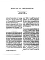
Adaptive Traffic Signal Control Using Fuzzy Logic

Adaptive Traffic Signal Control Using
Fuzzy
Logic
Stephen Chiu and
Sujeet
Chand
Rockwell International Science Center
1049
Camino
Dos
Rim
Thousand
Oaks,
CA
91360,
USA
Abstract

We present a distributed approach to traffic
signal control, where the signal timing parameters at a given
intersection are adjusted as functions of the local traffc
condition and of the signal timing parameters at adjacent
intersections. Thus, the signal timing parameters evolve
dynamically using only local information to improve trafic
flow.
This
distributed approach provides
for
a fault-tolerant,
highly responsive trafic management system.
The signal timing at an intersection is defined by three

parameters: cycle time, phase split,
and
offset. We use fuzzy
decision rules to adjust these three parameters based only on
local information. The amount of change in the timing
parameters during each cycle
is
limited to a
small
fraction of
the current parameters to ensure smooth transition. We show
the
effectiveness of this method through simulation
of
the
traffic
flow
in a network of controlled intersections.
I.
INTRODUCTION
With the steady increase
in
the number of automobiles on the
road, it has become ever more important
to
manage traffic
flow efficiently
to
optimize utilization of existing
road

capacity. High fuel cost and environmental concems also
provide important incentives for minimizing traffic delays.
To this end, computer technology
has
been
widely applied
to
optimize aaffic signal timing
to
facilitate traffic movement.
Traffic
signals
in use today typically operate
based
on a preset
timing schedule. The most common traffic control system
used in the United States is the Urban Traffic Control System
(UTCS),
developed by
the
Federal Highway Administration
in
the
1970s.
The
UTCS
generates timing schedules off-line on
a central computer based on average traffic conditions for a
specific time of day; the schedules are then downloaded to
the

local controllers at the corresponding time
of
day.
The
timing schedules are typically obtained by either maximizing
the bandwidth on arterial streets
or
minimizing a disutility
index that is generally a measure of delay and stops.
Computer
programs
such
as
MAXBAND
[13
and
TRANSYT-
7F
171
are well established means for performing these
optimizations.
0-7803-0614-7/93/$03.00 01993
IEEE
1371
The
off-line, global optimization approach
used
by
UTCS
cannot

respond
adequately
to
unpredictable
changes
in
traEfic
demand. With the availability of inexpensive
microprocessors, several
real-time
adaptive baffic control
systems were developed
in
the late
70's
and early
80's
to
address this problem. These systems
can
respond
to
changing
traffic demand by performing incremental
optimizations
at
the
local level. The most notable of these
are
SCATS

[2,3,61.
developed in Australia, and SCOOT
[3,5],
developed in
England. SCATS is installed in several major cities in
Australia, New Zealand, and
parts
of
Ask
recently the first
installation of SCATS
in
the U.S. was completed near
Detroit, Michigan. SCOOT is installed in over
40
cities, of
which
8
are
outside of England.
Both SCATS and SCOOT incrementally optimize the
signals' cycle
time,
phase split, and offset. The cycle time
is
the duration for completing all phases of a
signal;
phase split
is the division of the cycle time into
periods

of
green
signal
for competing approaches; offset
is
the
time
relationship
between the
start
of each phase among adjacent intersections.
SCATS organizes groups of intersections into subsystems.
Each subsystem contains only one critical intersection whose
timing parameters
are
adjusted
directly
by a
regional
computer
based
on the average prevailing traffic condition for the
area.
All other intersections in the subsystem are always
coordinated with the critical intersection, sharing
a
common
cycle time
and
coardinated phase

split
and
offset.
Subsystems
may
be
linked
to
form a
larger
coofdinated system
when
their
cycle times
are
nearly equal. At the lower level, each
intersection can independently shorten
or
omit a
particular
phase based
on
local traffic demand; however, any
time
saved
by ending a
phase
early must
be
added

to
the subsequent
phax
to maintain a common cycle time among all intersections in
the subsystem. The basic traffic data
used
by SCATS
is
the
"degree of saturation", defined
as
the
ratio
of the effectively
used green time
to
the
total
available green time. Cycle time
for a critical intersection is adjusted
to
maintain a high
degree
of saturation for the lane with the greatest degree
of
saturation. Phase split for a critical intersection
is
adjusted
to
maintain equal degrees of saturation on competing

approaches. The offsets among the intersections
in
a
subsystem
are
selected
to
minimize
stops
in the direction of
dominant traffic flow. Technical details are not available
from literature on exactly how
the
cycle
time
and phase split
of a critical intersection are adjusted. It seems that SCATS
does not explicitly optimize any specific performance
measure, such
as
average delay or stops.
SCOOT uses real-time traffic data
to
obtain traffic flow
models, called "cyclic flow profiles", on-line. The cyclic
flow profiles
are
then used
to
estimate how many vehicles

will arrive at a downstream signal when the signal is red.
This estimate provides predictions of queue size for different
hypothetical changes in the signal timing parameters.
SCOOTS objective is to minimize the sum of the average
queues in an
area.
A few seconds before every phase change,
SCOOT uses the flow model to determine whether it is better
to delay or advance the time of the phase change by
4
seconds, or leave it unaltered. Once a cycle, a similar
question is asked to determine whether the offset should
be
set
4
seconds earlier or later. Once every few minutes, a similar
question is asked to determine whether
the
cycle time should
be incremented or decremented by a few seconds. Thus,
SCOOT changes its timing parameters in fixed increments
to
optimize
an
explicit performance objective.
It is problematic that a specific performance objective will
be
appropriate for all traffic conditions. For example,
maximizing bandwidth on arterial streets may cause extended
wait time for vehicles on minor

streets.
On
the other hand,
minimizing delay and stops generally does not result in
maximum bandwidth. This problem is typically addressed by
the
use
of weighting factors; the
TRANSYT
optimization
program provides user-selectable link-to-link flow weighting,
stop weighting factors, and delay weighting factors.
A
traffic
engineer can vary these weighting factors until the program
produces a good
(by
human judgement) compromise solution.
Perhaps a performance index should be a function of the
traffic condition; it may be appropriate to emphasize
an
equitable distribution of movement opportunities when traffic
volume is low and emphasize overall network efficiency when
the traffic is congested.
In
view of the uncertainty in defining
a suitable performance measure, the reactive type of control
provided by
SCATS,
where there is no explicit effort to

optimize
any
specific performance measure, appears to have
merit. We believe implementing this type of control using
fuzzy logic decision rules can further enhance the
appropriateness of the control actions, increase control
flexibility, and produce performance characteristics that moce
closely match human's sensibility of "good" traffic
management.
In
past
work performed by Pappis and Mamdani
[4],
fuzzy
logic was applied to control an intersection of
two
one-way
streets.
It
was assumed that vehicle detectors were placed
sufficiently upstream from the intersection to inform the
controller about future
arrival
of vehicles at the intersection.
It
is then possible to predict the the number of vehicles that
will cross the intersection and the size of the queue that will
accumulate if no change to the the signal state takes place in
the next
N

seconds, for
N
=
1,2,

10.
The predicted
outcomes are evaluated by fuzzy decision rules to determine
the desirability of extending the current state for
N
more
seconds. Each of the possible extensions is assigned a degree
of confidence by the rules, and the extension with maximum
confidence is selected for implementation. Before the
extended period ends, the rules
are
applied again
to
see
if
further extensions
are
desirable.
Here we apply fuzzy logic to the general problem of
controlling multiple intersections in a network of two-way
streets. We propose a highly distributed architecture in which
each intersection independently adjusts its cycle time, phase
split, and offset using only local traffic
data
collected at the

intersection. This architecture provides for a fault-tolerant
traffic management system where traffic can
be
managed by
the collective actions
of
simple microprocessors located at
each intersection; hardware failure at a small number of
intersections should have minimal effect on overall network
performance. By requiring only local traffic data for
operation, the controllers can
be
installed individually and
incrementally into an area with existing signal controllers.
Each intersection
uses
an identical set of fuzzy decision rules
to adjust
its
timing parameters. The rules for adjusting the
cycle time and phase split follow the same general principles
used by SCATS: cycle time is adjusted
to
maintain a good
degree of saturation and phase split is adjusted
to
achieve
equal degrees of saturation on competing approaches. The
offset at each intersection is adjusted incrementally to
coordinate with the adjacent upstream intersection to

minimize stops in the direction of dominant traffic flow.
Through simulation
of
a small network of streets, the
distributed fuzzy control system has shown
to
be
effective in
rapidly reducing delay
and
stops.
II.
TRAFFIC
CONTROL
RULES
A
set of
40
fuzzy decision rules was used for adjusting the
signal timing parameters. The rules for adjusting cycle time,
phase split, and offset are decoupled
so
that
these
parameters
are adjusted independently; this greatly simplifies the rule
base. Although independent adjustment
of
these parameters
may result in one parameter change working against another,

no conflict was evident in simulations under various traffic
conditions. Since incremental adjustments
are
made
at
every
phase change, a conflicting adjustment will most likely
be
absorkd by the numerous successive adjustments.
A.
Cycle
Time
Adjustment
Cycle time is adjusted to maintain a good degree
of
saturation
on the approach with highest saturation. We define the degree
of saturation for a given approach
as
the actual number of
vehicles that passed through the intersection during the green
period divided by the maximum number of vehicles that can
pass through the intersection during that period.
Hence, the
degree of saturation is a measure of how effectively the green
period is being used. The primary reason for adjusting cycle
time
to
maintain
a given degree of saturation is not

to
ensure
1372
efficient use of green
periods,
but
to
control delay and stops.
When traffic volume is low, the cycle time must
be
reduced
to maintain a given degree of saturation; this
results
in
short
cycle times that reduce
the
delay
in
waiting for phase changes.
When the traffic volume is high, the cycle
time
must
be
increased to maintain the same degree
of
saturation; this
results in long cycle times that reduce the
numk
of

staps.
The rules for adjusting the cycle time
are
shown
in Fig.
1
and
the corresponding membership functions
are
shown
in Fig.
4.
The inputs to the rules are:
(1)
the highest degree of
saturation on any approach (denoted
as
"highest-sat" in the
rules), and
(2)
the highest degree of saturation
on
its
competing appmaches (denoted
as
"cross_sat"). The output of
the rules is the amount of adjustment
to
the current cycle
time, expressed

as
a fraction of the current cycle time. The
maximum adjustment allowed is
20%
of the current cycle
time. The rules basically adjust the cycle time in proportion
to the deviation
of
the degree of saturation from the desired
saturation value. However, when the highest saturation is
high and the saturation on the competing approach
is
low, we
can let the phase split adjustments alleviate the high
saturation. It should be noted that the "optimal" degree of
saturation
to
be
maintained by the controller is only
0.55,
whereas SCATS typically attempts
to
maintain a degree of
saturation of
0.9.
This discrepancy
arises
from
the method of
calculating the maximum (saturated) flow value. We derive

the
maximum
flow value
based
on a platoon
of
vehicles with
no gaps moving through the intersection at the
speed
limit,
while SCATS
uses
calibrated, more realistic values.
if
highest-sat is none
if
highest-sat is
low
if
highest-sat is slightly
low
if
highest-sat is
good
if highest-sat is high
6
cross-sat is not high
if highest-sat is high
6
cross-sat is high

if highest-sat is saturated
then cycl-change is n.big;
then cycl-change is n.med;
then cycl-change is n.sml;
then cycl-change is zero;
then cycl-change is p.sm1;
then cycl-change is p.med;
then cycl-change is p.big;
Fig.
I.
Rules
for
adjusting
cycle time.
B.
Phase Split Adjustment
Phase
split is adjusted
to
maintain equal degrees of saturation
on competing approaches. The rules for adjusting the phase
split is shown
in
Fig.
2
and the corresponding membership
functions
are
shown in Fig.
4.

The inputs
to
the rules
are:
(1)
the difference
between
the highest degree
of
saturation on
the east-west approaches and the highest degree of
saturation
on
the
north-south appmches ("sat-dW), and
(2)
the
highest
degree
of
saturation
on
any
approach ("highest-sat").
The
output
of
the
rules
is

the
amount of adjustment
to
the
current
east-west green
period,
expressed
as
a
fraction of
the
current
cycle time. Subaacting time from
the
w-west
green
Mod
is
equivalent
to
adding an
equal
amount
of
time
to
the
noRh-
south green

period.
When
the
saturation
difference
is large
and the highest degree of saturation
is
high,
the
green
period
is
adjusted
by
a
large amount
to
both
reduce
the
difference
and
alleviate the high saturation. When
the
highest degree of
saturation is low,
the
green
period

is
adjwted
by anly
a
small
amount to avoid excessive reduction in the degree of
saturation.
if
sat-diff is p.big
6
highest-sat is saturated
then green-change is p.biq;
if sat-diff is p.big
C
highest-sat is high
then green-change is p.big;
if sat-diff is p.big
6
highest-sat is not high
then green-change is p.med;
if sat-diff is n.big
6
highest-sat is saturated
then green-change is n.big;
if sat-diff is n.big
6
highest-sat is high
then green-change is n.big;
if sat-diff is n.big
6

highest-sat is not high
then green-change is n.med;
if sat-diff is p.med
&
highest-sat is saturated
then green-change is p.med;
if sat-diff is p.med
6
highest-sat is high
then green-change is p.med;
if sat-diff is p.med
6
highest-sat
is
not high
then green-change is
p.sml;
if sat-diff is n.med
6
highest-sat
is
saturated
then green-change is n.med;
if sat-diff is n.med
C
highest-sat
is
high
then green-change is n.med;
if sat-diff is n.med

6
highest-sat is not high
then green-change is n.sml;
if sat-diff is p.sml
then green-change is p.sml;
if sat-diff is n.sml
then green-change is n.sml;
if sat-diff is zero then green-change
is
zero;
Fig.
2.
Rules
for
adjusting
phase
split.
C.
Offset Adjustment
Offset is adjusted
to
coordinate adjacent signals in a way
that
minimizes stops
in
the direction of dominant
traffic
flow.
The controller first determines the dominant direction
from

the vehicle count for
each
approach.
Based
on the next green
time of the upstream intersection,
the
arrival
time of a vehicle
platoon leaving the upstream intersection can
be
calculated.
If
the local signal becomes green at that time, then the
vehicles will
pass
through the local intersection unstopped.
The required local adjustment
to
the time of
the
next phase
change is calculated based on this target green
time.
Fuzzy
rules are then applied to determine what fraction of the
1373
required adjustment can be reasonably executed in the current
cycle. The rules for determining the allowable adjustment
are

shown in Fig.
3
and the corresponding membership functions
are shown in Fig.
4.
The inputs
to
the rules
are:
(1) the
normalized difference between the traffic volume in the
dominant direction and the average volume in the remaining
directions ("vol-diff"); and
(2)
the required
time
adjustment
relative to the adjustable amount of time ("req-adjust"), e.g.,
the amount by which
the
current green phase is
to
be ended
early divided by the the current green period. The output of
the rules is the allowable adjustment, expressed
as
a fraction
of the required amount of adjustment. These rules will allow
a large fraction of the adjustment
to

be made if there is a
significant advantage to be gained by coordinating the flow in
the
dominant direction and that the adjustment
can
be made
without significant disruption
to
the current schedule.
if vol-diff is none
then allow-adjust is none;
if req-adjust is very.high
then allow-adjust is none;
if vol-diff is very.high
h
req-adjust is none
then allow-adjust is very high;
if vol-diff is very.high
6
req-adjust is low
then allow-adjust is very high;
if vol-diff is very.high
h
req-adjust is medium
then allow-adjust is high;
if vol-diff is very.high
h
req-adjust is high
then allow-adjust is medium;
if vol-diff is high

h
req-adjust
is
none
then allow-adjust is very high;
if vol-diff is high
&
req-adjust is .low
then allow-adjust is very high;
if vol-diff is high
h
req-adjust is medium
then allow-adjust is high;
if vol-diff
is
high
h
req-adjust is high
then allow-adjust is low;
if vol-diff is medium
6
req-adjust is none
then allow-adjust is very high;
if vol-diff is medium
&
req-adjust is low
then allow-adjust is high;
if
vol-diff is medium
h

req-adjust is medium
then allow-adjust is medium;
if vol-diff is medium
6
req-adjust is high
then allow-adjust is low;
if vol-diff is low
h
req-adjust is none
then allow-adjust is high;
if vol-diff is low
6
req-adjust is low
then allow-adjust is medium;
if vol-diff is low
h
req-adjust is medium
then allow-adjust is low;
if vol-diff is low
h
req-adjust is high
then allow-adjust is low;
Fig.
3.
Rules
for
adjusting
offset.
I
I

0.0
highestjd,
cross-sat
1
.o
I
I
-0.2
cycl-change, green-change
0.2
I
I
-0.5
sat-diff
0.5
I
I
0.0
vol-dlf,
re
q-adi
ust,
allow-adjust
1
.o
Fig.
4.
Membership
functions
used

in
des.
III.
SIMULATION RESULTS
Simulation was performed
to
verify the effectiveness of the
distributed fuzzy control scheme. We considered a small
network of intersections formed by six
streets,
shown in Fig.
5.
A mean vehicle arrival rate is assigned
to
each end of a
street. At every simulation time step, a random number is
generated for each lane of a street and compared with the
assigned vehicle arrival rate
to
determine whether a vehicle
should be added to the beginning of the lane. Some
simplifying assumptions were
used
in the simulation model:
(1)
unless stopped, a vehicle always moves at the speed
prescribed by the
speed
limit of
the

street,
(2)
a
vehicle cannot
change lane, and
(3)
a vehicle cannot
turn.
Vehicle counters
are assumed to be installed in all lanes of a street at each
intersection. When the the green phase begins for a given
approach, the number
of
vehicles passing through the
intersection during the green period
is
counted. The degree of
saturation for each approach is then calculated from the
vehicle count and the length of the green
period.
At the
start
of each phase change, the controller computes the time of the
next phase change using its current cycle time and phase split
values. The fuzzy decision rules
are
then applied
to
adjust the
time

of
the next phase change according to the offset
adjustment rules; the adjusted cycle time and phase split
values
are
used only
in
the subsequent computation of the
next phase change time.
1374
SOW
whh
+
1
I
I
I
It
I
Fig.
5.
Network
of
streets used in simulation.
Figure
6
shows the average waiting time
per
vehicle per
second spent in the network

as
a function -of time. Figure
7
shows the number of stops per minute encountered by all
vehicles. For the first
30
minutes of this simulation, all
intersections have a fixed cycle time of
40
seconds, a
green
duration of
20
seconds, and
start
their phases at the same
time. At the end of
30
minutes, intersections A,
B,
and
C
shown in Fig.
5
were allowed to adapt their timing
parameters according
to
the fuzzy decision rules. At the end
of
60

minutes, all intersections were allowed
to
adapt.
We
see that the improvement in waiting time is minimal when
only
3
intersections are adaptive. Furthermore, when only
3
intersections
are
adaptive, the minor improvement
in
waiting
time was obtained at the expense of greatly increased number
of stops. This
is
because the cycle time chosen by the
adaptive intersections (around
20
sec)
is widely different from
the cycle time for the fixed intersections
(40
sec). The
mismatch of cycle times resulted in a complete lack of
coordination between the adaptive intersections and the fixed
intersections, where timing adjustments to facilitate local
traffic movement can adversely affect the overall traffic
movement. When

all
intersections were allowed
to
adapt,
all
intersections auained similar cycle times (around
20
sec),
and
significant reductions in
both
waiting time and number of
stops were achieved.
Fig.
6.
Average waiting
time
for
the case in which all
intersections have
an
initial cycle time
of40
seconds.
Ipc,
U
I
I
800
"Olw

I
I
I
I
I
,
I
I
.I
I
Sintnections
I
I
J.)t
I
I
I
I
I
so
I I
I
OY)P~~OS)~O~DIDPD
Fig.
7.
Number
of
stops
for
the case in which all

intersections
have
an
initial cycle time
of40
seconds.
Tkc
(nk)
Figures
8
and
9
show the results of a simulation performed
using the
same
sequence of events, but with an initial cycle
time of
20
seconds and
green
duration
of
10
seconds
for
all
intersections.
In
this case, significant reductions in both
waiting time and number of

stops
were
achieved even
when
only
3
intersections
are
adaptive. This is because
the
cycle
time for the fixed intersections closely matches
that
chosen by
the adaptive intersections. Sharing a common cycle time
has
enabled the
3
adaptive intersections
to
have immediate positive
effect on overall system
performance.
1375
0
.ss
I
I
I
There

is
much that can
be
done
to
further
improve the present
fuzzy controller, such
as
including queue length
as
an
input
and using trend
data
for predictive control. The flexibility of
fuzzy decision rules greatly simplifies these extensions.
0.3
I
dlinttrsections
0.25-
0.2
-
d
intcrscctians
rt
I
REFERENCES
20
sec

cycletint,
I
3interseetions
I
1. Little,
J.,
Kelson, M. and Gartner,
N.
(1981).
MAXBAND:
A
Program
for Setting Signals on
Arteries
,,
;
;;o
;o
S,
&
&
i
and Triangular Networks.
Transportation Research
Record
795. National Research Council, Washington,
D.C., pp. 40-46.
0.15.
IDsccgrrtn
,

dDpt
0.1
Time
(nin)
Fig.
8.
Average waiting time
for
the Case in which all
intersections have an initial cycle time
of
20
seconds.
2.
bwrie,
p.
(1990). SCATS
-
A Traffic Responsive
Method of Controlling Urban Traffic. Sales information
brochure published by Roads
&
Traffic Authority,
Sydney, Australia.
3.
Luk,
J.
(1984). Two traffic-responsive
area
traffic

control methods: SCATS and SCOOT.
Traffic
Engineering
and
Control,
pp. 14-20.
4. Pappis, C. and Mamdani, E. (1977).
A
fuzzy logic
controller for a traffic junction.
IEEE Trans. Syst.,
Man, Cybern.
Vol. SMC-7,
No.
10.
5.
Robertson, D. and Bretherton,
R.
D. (1991).
Optimizing networks of traffic signals in
real
time
-
the
SCOOT method.
IEEE Trans. on Vehicular
Technology.
Vol. 40, No. 1, pp. 11-15.
Time
(mh)

6. Sims,
A.
(1979). The Sydney Coordinated Adaptive
Traffic System.
Proc. AXE Engineering Foundarion
Conference on Research Priorities in Computer Control
of
Urban Trafic Systems,
pp. 12-27.
Fig.
9.
Number
of
stops
for
the case in which all
intersections have an initial cycle time
of
20
seconds.
7. Wallace. C. et.
al.
(1988). TRANSYT-7F User’s Manual
Iv.
CONCLUDING
REMARKS
We have investigated the use of fuzzy decision rules for
adaptive traffic control.
A
highly distributed architecture

was
considered, where the timing parameters at each intersection
are
adjusted using only local information and coordinated only
with adjacent intersections. Although
this
localized approach
simplifies incremental integration of the fuzzy controller into
existing systems, simulation results show that the
effectiveness of a small number of “smart” intersections is
limited
if
they operate at a cycle time widely different from
the rest of the system. In this case, constraining the
controller to maintain a fixed cycle time that matches the
existing system may provide better overall performance. For
the case
in
which all intersections are adaptive, we need to
investigate whether better performance is achieved by
constraining all intersections to share a common variable
cycle time.
1376
(Releak 6). Prepared for F’HWA by the Transportation
Research Center, University of
Florida,
Gainesville,
FL.