starck, murtagh, fadili - sparse image and signal processing

Sparse Image and Signal Processing:
Wavelets, Curvelets, Morphological Diversity
This book presents the state of the art in sparse and multiscale image and signal process-
ing, covering linear multiscale transforms, such as wavelet, ridgelet, or curvelet trans-
forms, and non-linear multiscale transforms based on the median and mathematical
morphology operators. Recent concepts of sparsity and morphological diversity are de-
scribed and exploited for various problems such as denoising, inverse problem regular-
ization, sparse signal decomposition, blind source separation, and compressed sensing.
This book weds theory and practice in examining applications in areas such as astron-
omy, biology, physics, digital media, and forensics. A final chapter explores a paradigm
shift in signal processing, showing that previous limits to information sampling and
extraction can be overcome in very significant ways.
MATLAB and IDL code accompany these methods and applications to reproduce
the experiments and illustrate the reasoning and methodology of the research available
for download at the associated Web site.
Jean-Luc Starck is Senior Scientist at the Fundamental Laws of the Universe Research
Institute, CEA-Saclay. He holds a PhD from the University of Nice Sophia Antipolis and
the Observatory of the C
ˆ
ote d’Azur, and a Habilitation from the University of Paris 11.
He has held visiting appointments at the European Southern Observatory, the Univer-
sity of California Los Angeles, and the Statistics Department, Stanford University. He
is author of the following books: Image Processing and Data Analysis: The Multiscale
Approach and Astronomical Image and Data Analysis. In 2009, he won a European
Research Council Advanced Investigator award.
Fionn Murtagh directs Science Foundation Ireland’s national funding programs in In-
formation and Communications Technologies, and in Energy. He holds a PhD in Math-
ematical Statistics from the University of Paris 6, and a Habilitation from the Univer-
sity of Strasbourg. He has held professorial chairs in computer science at the University
of Ulster, Queen’s University Belfast, and now in the University of London at Royal

Holloway. He is a Member of the Royal Irish Academy, a Fellow of the International
Association for Pattern Recognition, and a Fellow of the British Computer Society.
Jalal M. Fadili graduated from the
´
Ecole Nationale Sup
´
erieure d’Ing
´
enieurs (ENSI),
Caen, France, and received MSc and PhD degrees in signal processing, and a Habilita-
tion, from the University of Caen. He was McDonnell-Pew Fellow at the University of
Cambridge in 1999–2000. Since 2001, he is Associate Professor of Signal and Image Pro-
cessing at ENSI. He has held visiting appointments at Queensland University of Tech-
nology, Stanford University, Caltech, and EPFL.

SPARSE IMAGE AND
SIGNAL PROCESSING
Wavelets, Curvelets,
Morphological Diversity
Jean-Luc Starck
Centre d’
´
Etudes de Saclay, France
Fionn Murtagh
Royal Holloway, University of London
Jalal M. Fadili
´
Ecole Nationale Sup
´
erieure d’Ing

´
enieurs, Caen
cambridge university press
Cambridge, New York, Melbourne, Madrid, Cape Town, Singapore,
S
˜
ao Paulo, Delhi, Dubai, Tokyo
Cambridge University Press
32 Avenue of the Americas, New York, NY 10013-2473, USA
www.cambridge.org
Information on this title: www.cambridge.org/9780521119139
C

Jean-Luc Starck, Fionn Murtagh, and Jalal M. Fadili 2010
This publication is in copyright. Subject to statutory exception
and to the provisions of relevant collective licensing agreements,
no reproduction of any part may take place without the written
permission of Cambridge University Press.
First published 2010
Printed in the United States of America
A catalog record for this publication is available from the British Library.
Library of Congress Cataloging in Publication data
Starck, J L. (Jean-Luc), 1965–
Sparse image and signal processing : wavelets, curvelets, morphological
diversity / Jean-Luc Starck, Fionn Murtagh, Jalal Fadili.
p. cm.
Includes bibliographical references and index.
ISBN 978-0-521-11913-9 (hardback)
1. Transformations (Mathematics) 2. Signal processing. 3. Image processing.
4. Sparse matrices. 5. Wavelets (Mathematics) I. Murtagh, Fionn. II. Fadili,

Jalal, 1973– III. Title.
QA601.S785 2010
621.36

7–dc22 2009047391
ISBN 978-0-521-11913-9 Hardback
Additional resources for this publication at www.SparseSignalRecipes.info
Cambridge University Press has no responsibility for the persistence or
accuracy of URLs for external or third-party Internet Web sites referred to in
this publication and does not guarantee that any content on such Web sites is,
or will remain, accurate or appropriate.
Contents
Acronyms page ix
Notation xiii
Preface xv
1 Introduction to the World of Sparsity . . . . 1
1.1 Sparse Representation 1
1.2 From Fourier to Wavelets 5
1.3 From Wavelets to Overcomplete Representations 6
1.4 Novel Applications of the Wavelet and Curvelet Transforms 8
1.5 Summary 15
2 The Wavelet Transform . 16
2.1 Introduction 16
2.2 The Continuous Wavelet Transform 16
2.3 Examples of Wavelet Functions 18
2.4 Continuous Wavelet Transform Algorithm 21
2.5 The Discrete Wavelet Transform 22
2.6 Nondyadic Resolution Factor 28
2.7 The Lifting Scheme 31
2.8 Wavelet Packets 34

2.9 Guided Numerical Experiments 38
2.10 Summary 44
3 Redundant Wavelet Transfor m . . . 45
3.1 Introduction 45
3.2 The Undecimated Wavelet Transform 46
3.3 Partially Decimated Wavelet Transform 49
3.4 The Dual-Tree Complex Wavelet Transform 51
3.5 Isotropic Undecimated Wavelet Transform: Starlet Transform 53
3.6 Nonorthogonal Filter Bank Design 58
3.7 Pyramidal Wavelet Transform 64
v
vi Contents
3.8 Guided Numerical Experiments 69
3.9 Summary 74
4 Nonlinear Multiscale Transforms . 75
4.1 Introduction 75
4.2 Decimated Nonlinear Transform 75
4.3 Multiscale Transform and Mathematical Morphology 77
4.4 Multiresolution Based on the Median Transform 81
4.5 Guided Numerical Experiments 86
4.6 Summary 88
5 The Ridgelet and Curvelet Transforms 89
5.1 Introduction 89
5.2 Background and Example 89
5.3 Ridgelets 91
5.4 Curvelets 100
5.5 Curvelets and Contrast Enhancement 110
5.6 Guided Numerical Experiments 112
5.7 Summary 118
6 SparsityandNoiseRemoval 119

6.1 Introduction 119
6.2 Term-By-Term Nonlinear Denoising 120
6.3 Block Nonlinear Denoising 127
6.4 Beyond Additive Gaussian Noise 132
6.5 Poisson Noise and the Haar Transform 134
6.6 Poisson Noise with Low Counts 136
6.7 Guided Numerical Experiments 143
6.8 Summary 145
7 Linear Inverse Problems . 149
7.1 Introduction 149
7.2 Sparsity-Regularized Linear Inverse Problems 151
7.3 Monotone Operator Splitting Framework 152
7.4 Selected Problems and Algorithms 160
7.5 Sparsity Penalty with Analysis Prior 170
7.6 Other Sparsity-Regularized Inverse Problems 172
7.7 General Discussion: Sparsity, Inverse Problems, and Iterative
Thresholding 174
7.8 Guided Numerical Experiments 176
7.9 Summary 178
8 Morphological Diversity . . 180
8.1 Introduction 180
8.2 Dictionary and Fast Transformation 183
8.3 Combined Denoising 183
8.4 Combined Deconvolution 188
8.5 Morphological Component Analysis 190
Contents vii
8.6 Texture-Cartoon Separation 198
8.7 Inpainting 204
8.8 Guided Numerical Experiments 210
8.9 Summary 216

9 Sparse Blind Source Separation . . 218
9.1 Introduction 218
9.2 Independent Component Analysis 220
9.3 Sparsity and Multichannel Data 224
9.4 Morphological Diversity and Blind Source Separation 226
9.5 Illustrative Experiments 237
9.6 Guided Numerical Experiments 242
9.7 Summary 244
10 Multiscale Geometric Analysis on the Sphere 245
10.1 Introduction 245
10.2 Data on the Sphere 246
10.3 Orthogonal Haar Wavelets on the Sphere 248
10.4 Continuous Wavelets on the Sphere 249
10.5 Redundant Wavelet Transform on the Sphere with Exact
Reconstruction 253
10.6 Curvelet Transform on the Sphere 261
10.7 Restoration and Decomposition on the Sphere 266
10.8 Applications 269
10.9 Guided Numerical Experiments 272
10.10 Summary 276
11 CompressedSensing 277
11.1 Introduction 277
11.2 Incoherence and Sparsity 278
11.3 The Sensing Protocol 278
11.4 Stable Compressed Sensing 280
11.5 Designing Good Matrices: Random Sensing 282
11.6 Sensing with Redundant Dictionaries 283
11.7 Compressed Sensing in Space Science 283
11.8 Guided Numerical Experiments 285
11.9 Summary 286

References 289
List of Algorithms 311
Index 313
Color Plates follow page 148

Acronyms
1-D, 2-D, 3-D one-dimensional, two-dimensional, three-dimensional
AAC advanced audio coding
AIC Akaike information criterion
BCR block-coordinate relaxation
BIC Bayesian information criterion
BP basis pursuit
BPDN basis pursuit denoising
BSS blind source separation
CCD charge-coupled device
CeCILL CEA CNRS INRIA Logiciel Libre
CMB cosmic microwave background
COBE Cosmic Background Explorer
CTS curvelet transform on the sphere
CS compressed sensing
CWT continuous wavelet transform
dB decibel
DCT discrete cosine transform
DCTG1, DCTG2 first-generation discrete curvelet transform, s econd-
generation discrete curvelet transform
DR Douglas-Rachford
DRT discrete ridgelet transform
DWT discrete wavelet transform
ECP equidistant coordinate partition
EEG electroencephalography

EFICA efficient fast independent component analysis
EM expectation maximization
ERS European remote sensing
ESA European Space Agency
FB forward-backward
FDR false discovery rate
FFT fast Fourier transform
ix
x Acronyms
FIR finite impulse response
FITS Flexible Image Transport System
fMRI functional magnetic resonance imaging
FSS fast slant stack
FWER familywise error rate
FWHM full width at half maximum
GCV generalized cross-validation
GGD generalized Gaussian distribution
GLESP Gauss-Legendre sky pixelization
GMCA generalized morphological component analysis
GUI graphical user interface
HEALPix hierarchical equal area isolatitude pixelization
HSD hybrid steepest descent
HTM hierarchical triangular mesh
ICA independent component analysis
ICF inertial confinement fusion
IDL interactive data language
IFFT inverse fast Fourier transform
IHT iterative hard thresholding
iid independently and identically distributed
IRAS Infrared Astronomical Satellite

ISO Infrared Space Observatory
IST iterative soft thresholding
IUWT isotropic undecimated wavelet (starlet) transform
JADE joint approximate diagonalization of eigen-matrices
JPEG Joint Photographic Experts Group
KL Kullback-Leibler
LARS least angle regression
LP linear programming
lsc lower semicontinuous
MAD median absolute deviation
MAP maximum a posteriori
MCA morphological component analysis
MDL minimum description length
MI mutual information
ML maximum likelihood
MMSE minimum mean squares estimator
MMT multiscale median transform
MMV multiple measurements vectors
MOLA Mars Orbiter Laser Altimeter
MOM mean of maximum
MP matching pursuit
MP3 MPEG-1 Audio Layer 3
MPEG Moving Picture Experts Group
MR magnetic resonance
MRF Markov random field
MSE mean square error
Acronyms xi
MS-VST multiscale variance stabilization transform
NLA nonlinear approximation
OFRT orthonormal finite ridgelet transform

OMP orthogonal matching pursuit
OSCIR Observatory Spectrometer and Camera for the Infrared
OWT orthogonal wavelet transform
PACS Photodetector Array Camera and Spectrometer
PCA principal components analysis
PCTS pyramidal curvelet transform on the sphere
PDE partial differential equation
pdf probability density function
PMT pyramidal median transform
POCS projections onto convex sets
PSF point spread function
PSNR peak signal-to-noise ratio
PWT partially decimated wavelet transform
PWTS pyramidal wavelet transform on the sphere
QMF quadrature mirror filters
RIC restricted isometry constant
RIP restricted isometry property
RNA relative Newton algorithm
SAR Synthetic Aperture Radar
SeaWiFS Sea-viewing Wide Field-of-view Sensor
SNR signal-to-noise ratio
s.t. subject to
STFT short-time Fourier transform
StOMP Stage-wise Orthogonal Matching Pursuit
SURE Stein unbiased risk estimator
TV total variation
UDWT undecimated discrete wavelet transform
USFFT unequispaced fast Fourier transform
UWT undecimated wavelet transform
UWTS undecimated wavelet transform on the sphere

VST variance-stabilizing transform
WMAP Wilkinson Microwave Anisotropy Probe
WT wavelet transform

Notation
Functions and Signals
f (t) continuous-time function, t ∈ R
f (t)or f (t
1
, ,t
d
) d-dimensional continuous-time function, t ∈ R
d
f [k] discrete-time signal, k ∈ Z,orkth entry of a
finite-dimensional vector
f [k]or f [k, l, ] d-dimensional discrete-time signal, k ∈ Z
d
¯
f time-reversed version of f as a function
(
¯
f (t) = f (−t), ∀t ∈ R) or signal
(
¯
f [k] = f [−k], ∀k ∈ Z)
ˆ
f Fourier transform of f
f
∗
complex conjugate of a function or signal

H(z) z transform of a discrete filter h
lhs = O(rhs) lhs is of order rhs; there exists a constant C > 0 such that
lhs ≤ Crhs
lhs ∼ rhs lhs is equivalent to rhs; lhs = O(rhs) and rhs = O(lhs)
1
{condition}
1 if condition is met, and zero otherwise
L
2
() space of square-integrable functions on a continuous
domain 

2
() space of square-summable signals on a discrete domain 

0
(H) class of proper lower-semicontinuous convex functions
from H to R ∪{+∞}
Operators on Signals or Functions
[·]
↓2
down-sampling or decimation by a f actor 2
[·]
↓2
e
down-sampling by a factor 2 that keeps even samples
[·]
↓2
o
down-sampling by a factor 2 that keeps odd samples

˘. or [·]
↑2
up-sampling by a factor 2, i.e., zero insertion between
each two samples
[·]
↑2
e
even-sample zero insertion
[·]
↑2
o
odd-sample zero insertion
xiii
xiv Notation
[·]
↓2,2
down-sampling or decimation by a factor 2 in each
direction of a two-dimensional image
∗ continuous convolution
 discrete convolution
 composition (arbitrary)
Matrices, Linear Operators, and Norms
·
T
transpose of a vector or a matrix
M
∗
adjoint of M
Gram matrix of MM
∗

M or M
T
M
M[i, j] entry at ith row and jth column of a matrix M
det(M) determinant of a matrix M
rank(M) rank of a matrix M
diag(M) diagonal matrix with the same diagonal elements as its
argument M
trace(M) trace of a square matrix M
vect(M) stacks the columns of M in a long column vector
M
+
pseudo-inverse of M
I identity operator or identity matrix of appropriate
dimension; I
n
if the dimension is not clear from the
context

·, ·

inner product (in a pre-Hilbert space)

·

associated norm

·

p

p ≥ 1, 
p
norm of a signal

·

0

0
quasi-norm of a signal; number of nonzero elements

·

TV
discrete total variation (semi)norm
∇ discrete gradient of an image
div discrete divergence operator (adjoint of ∇)
||| · ||| spectral norm for linear operators

·

F
Frobenius norm of a matrix
⊗ tensor product
Random Variables and Vectors
ε ∼ N (μ, ) ε is normally distributed with mean μ and covariance 
ε ∼ N (μ, σ
2
) ε is additive white Gaussian with mean μ and variance σ
2

ε ∼ P(λ) ε is Poisson distributed with intensity (mean) λ
E[.] expectation operator
Var[.] variance operator
φ(ε; μ, σ
2
) normal probability density function of mean μ and
variance σ
2
Φ(ε; μ, σ
2
) normal cumulative distribution of mean μ and
variance σ
2
Preface
Often, nowadays, one addresses public understanding of mathematics and rigor by
pointing to important applications and how they underpin a great deal of science
and engineering. In this context, multiple resolution methods in image and signal
processing, as discussed in depth in this book, are important. Results of such meth-
ods are often visual. Results, too, can often be presented to the layperson in an easily
understood way. In addition to those aspects that speak powerfully in favor of the
methods presented here, the following is worth noting. Among the most cited arti-
cles in statistics and signal processing, one finds works in the general area of what
we cover in this book.
The methods discussed in this book are essential underpinnings of data analysis,
of relevance to multimedia data processing and to image, video, and signal process-
ing. The methods discussed here feature very crucially in statistics, in mathematical
methods, and in computational techniques.
Domains of application are incredibly wide, including imaging and signal pro-
cessing in biology, medicine, and the life sciences generally; astronomy, physics, and
the natural sciences; seismology and land use studies, as indicative subdomains from

geology and geography in the earth sciences; materials science, metrology, and other
areas of mechanical and civil engineering; image and video compression, analysis,
and synthesis for movies and television; and so on.
There is a weakness, though, in regard to well-written available works in this
area: the very rigor of the methods also means that the ideas can be very deep.
When separated from the means to apply and to experiment with the methods, the
theory and underpinnings can require a great deal of background knowledge and
diligence – and study, too – to grasp the essential material.
Our aim in this book is to provide an essential bridge between theoretical back-
ground and easily applicable experimentation. We have an additional aim, namely,
that coverage be as extensive as can be, given the dynamic and broad field with
which we are dealing.
Our approach, which is wedded to theory and practice, is based on a great deal
of practical engagement across many application areas. Very varied applications
are used for illustration and discussion in this book. This is natural, given how
xv
xvi Preface
ubiquitous the wavelet and other multiresolution transforms have become. These
transforms have become essential building blocks for addressing problems across
most of data, signal, image, and indeed information handling and processing. We
can characterize our approach as premised on an embedded systems view of how
and where wavelets and multiresolution methods are to be used.
Each chapter has a section titled “Guided Numerical Experiments,” comple-
menting the accompanying description. In fact, these sections independently pro-
vide the reader with a set of recipes for quick and easy trial and assessment of the
methods presented. Our bridging of theory and practice uses openly accessible and
freely available as well as very widely used MATLAB toolboxes. In addition, inter-
active data language is used, and all code described and used here is freely available.
The scripts that we discuss in this book are available online (http://www.
SparseSignalRecipes.info) together with the sample images used. In this form, the

software code is succinct and easily shown in the text of the book. The code caters to
all commonly used platforms: Windows, Macintosh, Linux, and other Unix systems.
In this book, we exemplify the theme of reproducible research. Reproducibility
is at the heart of the scientific method and all successful technology development. In
theoretical disciplines, the gold standard has been set by mathematics, where formal
proof, in principle, allows anyone to reproduce the cognitive steps leading to verifi-
cation of a theorem. In experimental disciplines, such as biology, physics, or chem-
istry, for a result to be well established, particular attention is paid to experiment
replication. Computational science is a much younger field than mathematics but
is already of great importance. By reproducibility of research, here it is recognized
that the outcome of a research project is not just publication, but rather the en-
tire environment used to reproduce the results presented, including data, software,
and documentation. An inspiring early example was Don Knuth’s seminal notion of
literate programming, which he developed in the 1980s to ensure trust or even un-
derstanding for software code and algorithms. In the late 1980s, Jon Claerbout, of
Stanford University, used the Unix Make tool to guarantee automatic rebuilding of
all results in a paper. He imposed on his group the discipline that all research books
and publications originating from his group be completely reproducible.
In computational science, a paradigmatic end product is a figure in a paper. Un-
fortunately, it is rare that the reader can attempt to rebuild the authors’ complex
system in an attempt to understand what the authors might have done over months
or years. Through our providing software and data sets coupled to the figures in this
book, the reader will be able to reproduce what we have here.
This book provides both a means to access the state of the art in theory and a
means to experiment through the software provided. By applying, in practice, the
many cutting-edge signal processing approaches described here, the reader will gain
a great deal of understanding. As a work of reference, we believe that this book will
remain invaluable for a long time to come.
The book is aimed at graduate-level study, advanced undergraduate study, and
self-study. The target reader includes whoever has a professional interest in image

and signal processing. Additionally, the target reader is a domain specialist in data
analysis in any of a very wide swath of applications who wants to adopt innova-
tive approaches in his or her field. A further class of target reader is interested in
learning all there is to know about the potential of multiscale methods and also in
Preface xvii
having a very complete overview of the most recent perspectives in this area. An-
other class of target reader is undoubtedly the student – an advanced undergradu-
ate project student, for example, or a doctoral student – who needs to grasp theory
and application-oriented understanding quickly and decisively in quite varied ap-
plication fields as well as in statistics, industrially oriented mathematics, electrical
engineering, and elsewhere.
The central themes of this book are scale, sparsity, and morphological diversity.
The term sparsity implies a form of parsimony. Scale is synonymous with resolution.
Colleagues we would like to acknowledge include Bedros Afeyan, Nabila
Aghanim, Albert Bijaoui, Emmanuel Cand
`
es, Christophe Chesneau, David Don-
oho, Miki Elad, Olivier Forni, Yassir Moudden, Gabriel Peyr
´
e, and Bo Zhang. We
would like to particularly acknowledge J
´
er
ˆ
ome Bobin, who contributed to the blind
source separation chapter. We acknowledge joint analysis work with the following,
relating to images in Chapter 1: Will Aicken, P. A. M. Basheer, Kurt Birkle, Adrian
Long, and Paul Walsh.
The cover art was designed by Aur
´

elie Bordenave ().
We thank her for this work.

1
Introduction to the World of Sparsity
We first explore recent developments in multiresolution analysis. Essential ter-
minology is introduced in the scope of our general overview, which includes the
coverage of sparsity and sampling, best dictionaries, overcomplete representation
and redundancy, compressed sensing and sparse representation, and morphological
diversity.
Then we describe a range of applications of visualization, filtering, feature detec-
tion, and image grading. Applications range over Earth observation and astronomy,
medicine, civil engineering and materials science, and image databases generally.
1.1 SPARSE REPRESENTATION
1.1.1 Introduction
In the last decade, sparsity has emerged as one of the leading concepts in a wide
range of signal-processing applications (restoration, feature extraction, source sepa-
ration, and compression, to name only a few applications). Sparsity has long been an
attractive theoretical and practical signal property in many areas of applied math-
ematics (such as computational harmonic analysis, statistical estimation, and theo-
retical signal processing).
Recently, researchers spanning a wide range of viewpoints have advocated the
use of overcomplete signal representations. Such representations differ from the
more traditional representations because they offer a wider range of generating ele-
ments (called atoms). Indeed, the attractiveness of redundant signal representations
relies on their ability to economically (or compactly) represent a large class of sig-
nals. Potentially, this wider range allows more flexibility in signal representation
and adaptivity to its morphological content and entails more effectiveness in many
signal-processing tasks (restoration, separation, compression, and estimation). Neu-
roscience also underlined the role of overcompleteness. Indeed, the mammalian vi-

sual system has been shown to be likely in need of overcomplete representation
(Field 1999; Hyv
¨
arinen and Hoyer 2001; Olshausen and Field 1996a; Simoncelli and
1
2 Introduction to the World of Sparsity
Olshausen 2001). In that setting, overcomplete sparse coding may lead to more ef-
fective (sparser) codes.
The interest in sparsity has arisen owing to the new sampling theory, compressed
sensing (also called compressive sensing or compressive sampling), which provides
an alternative to the well-known Shannon sampling theory (Cand
`
es and Tao 2006;
Donoho 2006a; Cand
`
es et al. 2006b). Compressed sensing uses the prior knowledge
that signals are sparse, whereas Shannon theory was designed for frequency band–
limited signals. By establishing a direct link between sampling and sparsity, com-
pressed sensing has had a huge impact in many scientific fields such as coding and
information theory, signal and image acquisition and processing, medical imaging,
and geophysical and astronomical data analysis. Compressed sensing acts today as
wavelets did two decades ago, linking researchers from different fields. Further con-
tributing to the success of compressed sensing is that some traditional inverse prob-
lems, such as tomographic image reconstruction, can be understood as compressed
sensing problems (Cand
`
es et al. 2006b; Lustig et al. 2007). Such ill-posed problems
need to be regularized, and many different approaches to regularization have been
proposed in the last 30 years (Tikhonov regularization, Markov random fields, to-
tal variation, wavelets, etc.). But compressed sensing gives strong theoretical sup-

port for methods that seek a sparse solution because such a solution may be (under
certain conditions) the exact one. Similar results have not been demonstrated with
any other regularization method. These reasons explain why, just a few years after
seminal compressed sensing papers were published, many hundreds of papers have
already appeared in this field (see, e.g., the compressed sensing resources Web site
).
By emphasizing so rigorously the importance of sparsity, compressed sensing has
also cast light on all work related to sparse data representation (wavelet transform,
curvelet transform, etc.). Indeed, a signal is generally not sparse in direct space (i.e.,
pixel space), but it can be very sparse after being decomposed on a specific set of
functions.
1.1.2 What Is Sparsity?
1.1.2.1 Strictly Sparse Signals/Images
A signal x, considered as a vector in a finite-dimensional subspace of R
N
, x =
[
x[1], ,x[N]
]
, is strictly or exactly sparse if most of its entries are equal to
zero, that is, if its support (x) ={1 ≤ i ≤ N | x[i] = 0} is of cardinality k  N .
A k-sparse signal is a signal for which exactly k samples have a nonzero value.
If a signal is not sparse, it may be sparsified in an appropriate transform domain.
For instance, if x is a sine, it is clearly not sparse, but its Fourier transform is ex-
tremely sparse (actually, 1-sparse). Another example is a piecewise constant image
away from edges of finite length that has a sparse gradient.
More generally, we can model a signal x as the linear combination of T elemen-
tary waveforms, also called signal atoms, such that
x = α =
T


i=1
α[i]ϕ
i
, (1.1)
1.1 Sparse Representation 3
where α[i] are called the representation coefficients of x in the dictionary  =
[ϕ
1
, ,ϕ
T
](theN × T matrix whose columns are the atoms ϕ
i
, in general nor-
malized to a unit 
2
norm, i.e., ∀i ∈{1, ,T },

ϕ
i

2
=

N
n=1
|ϕ
i
[n]|
2

= 1).
Signals or images x that are sparse in  are those that can be written exactly as a
superposition of a small fraction of the atoms in the family
(
ϕ
i
)
i
.
1.1.2.2 Compressible Signals/Images
Signals and images of practical interest are not, in general, strictly sparse. Instead,
they may be compressible or weakly sparse in the sense that the sorted magni-
tudes |α
(i)
| of the representation coefficients α = 
T
x decay quickly according to
the power law


α
(i)


≤ Ci
−1/s
, i = 1, ,T ,
and the nonlinear approximation error of x from its k-largest coefficients (denoted
x
k

) decays as

x − x
k

≤ C(2/s − 1)
−1/2
k
1/2−1/s
, s < 2.
In other words, one can neglect all but perhaps a small fraction of the coefficients
without much loss. Thus x can be well approximated as k-sparse.
Smooth signals and piecewise smooth signals exhibit this property in the wavelet
domain (Mallat 2008). Owing to recent advances in harmonic analysis, many redun-
dant systems, s uch as the undecimated wavelet transform, curvelet, and contourlet,
have been shown to be very effective in sparsely representing images. As popular
examples, one may think of wavelets for smooth images with isotropic singularities
(Mallat 1989, 2008), bandlets (Le Pennec and Mallat 2005; Peyr
´
e and Mallat 2007;
Mallat and Peyr
´
e 2008), grouplets (Mallat 2009) or curvelets for representing piece-
wise smooth C
2
images away from C
2
contours (Cand
`
es and Donoho 2001; Cand

`
es
et al. 2006a), wave atoms or local discrete cosine transforms to represent locally
oscillating textures (Demanet and Ying 2007; Mallat 2008), and so on. Compress-
ibility of signals and images forms the foundation of transform coding, which is the
backbone of popular compression standards in audio (MP3, AAC), imaging (JPEG,
JPEG-2000), and video (MPEG).
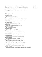
Figure 1.1 shows the histogram of an image in both the original domain (i.e.,
 = I, where I is the identity operator, hence α = x) and the curvelet domain. We
can see immediately that these two histograms are very different. The second his-
togram presents a typical sparse behavior (unimodal, sharply peaked with heavy
tails), where most of the coefficients are close to zero and few are in the tail of the
distribution.
Throughout the book, with a slight abuse of terminology, we may call signals and
images sparse, both those that are strictly sparse and those that are compressible.
1.1.3 Sparsity Terminology
1.1.3.1 Atom
As explained in the previous section, an atom is an elementary signal-representing
template. Examples include sinusoids, monomials, wavelets, and Gaussians. Using a
4 Introduction to the World of Sparsity
50 100 150 200
0
0.005
0.01
0.015
Gray level
30 20 10 0 10 20 30
0
0.5
1

1.5
Curvelet coefficient
Figure 1.1. Histogram of an image in (left) the original (pixel) domain and (right) the curvelet
domain.
collection of atoms as building blocks, one can construct more complex waveforms
by linear superposition.
1.1.3.2 Dictionary
A dictionary  is an indexed collection of atoms
(
ϕ
γ
)
γ ∈
, where  is a countable
set; that is, its cardinality
|

|
= T . The interpretation of the index γ depends on
the dictionary: frequency for the Fourier dictionary (i.e., sinusoids), position for the
Dirac dictionary (also known as standard unit vector basis or Kronecker basis), posi-
tion scale for the wavelet dictionary, translation-duration-frequency for cosine pack-
ets, and position-scale-orientation for the curvelet dictionary in two dimensions. In
discrete-time, finite-length signal processing, a dictionary is viewed as an N × T ma-
trix whose columns are the atoms, and the atoms are considered as column vectors.
When the dictionary has more columns than rows, T > N,itiscalledovercomplete
or redundant. The overcomplete case is the setting in which x = α amounts to an
underdetermined system of linear equations.
1.1.3.3 Analysis and Synthesis
Given a dictionary, one has to distinguish between analysis and synthesis operations.

Analysis is the operation that associates with each signal x a vector of coefficients
α attached to an atom: α = 
T
x.
1
Synthesis is the operation of reconstructing x by
1
The dictionary is supposed to be real. For a complex dictionary, 
T
is to be replaced by the conjugate
transpose (adjoint) 
∗
.
1.2 From Fourier to Wavelets 5
superposing atoms: x = α. Analysis and synthesis are different linear operations.
In the overcomplete case,  is not invertible, and the reconstruction is not unique
(see also Section 8.2 for further details).
1.1.4 Best Dictionary
Obviously, the best dictionary is the one that leads to the sparsest representation.
Hence we could imagine having a huge dictionary (i.e., T  N), but we would be
faced with a prohibitive computation time cost for calculating the α coefficients.
Therefore there is a trade-off between the complexity of our analysis (i.e., the size of
the dictionary) and computation time. Some specific dictionaries have the advantage
of having fast operators and are very good candidates for analyzing the data. The
Fourier dictionary is certainly the most well known, but many others have been
proposed in the literature such as wavelets (Mallat 2008), ridgelets (Cand
`
es and
Donoho 1999), curvelets (Cand
`

es and Donoho 2002; Cand
`
es et al. 2006a; Starck
et al. 2002), bandlets (Le Pennec and Mallat 2005), and contourlets (Do and Vetterli
2005), to name but a few candidates. We will present some of these in the chapters
to follow and show how to use them for many inverse problems such as denoising
or deconvolution.
1.2 FROM FOURIER TO WAVELETS
The Fourier transform is well suited only to the study of stationary signals, in which
all frequencies have an infinite coherence time, or, otherwise expressed, the signal’s
statistical properties do not change over time. Fourier analysis is based on global
information that is not adequate for the study of compact or local patterns.
As is well known, Fourier analysis uses basis functions consisting of sine and co-
sine functions. Their frequency content is time-independent. Hence the description
of the signal provided by Fourier analysis is purely in the frequency domain. Music
or the voice, however, imparts information in both the time and the frequency do-
mains. The windowed Fourier transform and the wavelet transform aim at an anal-
ysis of both time and frequency. A short, informal introduction to these different
methods can be found in the work of Bentley and McDonnell (1994), and further
material is covered by Chui (1992), Cohen (2003), and Mallat (2008).
For nonstationary analysis, a windowed Fourier transform (short-time Fourier
transform, STFT) can be used. Gabor (1946) introduced a local Fourier analysis,
taking into account a sliding Gaussian window. Such approaches provide tools for
investigating time and frequency. Stationarity is assumed within the window. The
smaller the window size, the better is the time resolution; however, the smaller the
window size, also, the more the number of discrete frequencies that can be repre-
sented in the frequency domain will be reduced, and therefore the more weakened
will be the discrimination potential among frequencies. The choice of window thus
leads to an uncertainty trade-off.
The STFT transform, for a continuous-time signal s(t), a window g around time

point τ , and frequency ω,is
STFT(τ,ω) =
+∞

−∞
s(t)g(t −τ)e
−j ωt
dt. (1.2)
6 Introduction to the World of Sparsity
Considering
k
τ,ω
(t) = g(t −τ)e
−j ωt
(1.3)
as a new basis, and rewriting this with window size a, inversely proportional to the
frequency ω, and with positional parameter b replacing τ ,as
k
b,a
(t) =
1
√
a
ψ
∗

t − b
a

, (1.4)

yields the continuous wavelet transform (CWT), where ψ
∗
is the complex conjugate
of ψ. In the STFT, the basis functions are windowed sinusoids, whereas in the CWT,
they are scaled versions of a so-called mother function ψ.
In the early 1980s, the wavelet transform was studied theoretically in geophysics
and mathematics by Morlet, Grossman, and Meyer. I n the late 1980s, links with
digital signal processing were pursued by Daubechies and Mallat, thereby putting
wavelets firmly into the application domain.
A wavelet mother function can take many forms, subject to some admissibility
constraints. The best choice of mother function for a particular application is not
given a priori.
From the basic wavelet formulation, one can distinguish (Mallat 2008) between
(1) the CWT, described earlier, and (2) the discrete wavelet transform, which dis-
cretizes the continuous transform but does not, in general, have an exact analytical
reconstruction formula; and within discrete transforms, distinction can be made be-
tween (3) redundant versus nonredundant (e.g., pyramidal) transforms and (4) or-
thonormal versus other bases of wavelets. The wavelet transform provides a decom-
position of the original data, allowing operations to be performed on the wavelet
coefficients, and then the data are reconstituted.
1.3 FROM WAVELETS TO OVERCOMPLETE REPRESENTATIONS
1.3.1 The Blessing of Overcomplete Representations
As discussed earlier, different wavelet transform algorithms correspond to different
wavelet dictionaries. When the dictionary is overcomplete, T > N, the number of
coefficients is larger than the number of signal samples. Because of the redundancy,
there is no unique way to reconstruct x from the coefficients α. For compression
applications, we obviously prefer to avoid this redundancy, which would require us
to encode a greater number of coefficients. But for other applications, such as image
restoration, it will be shown that redundant wavelet transforms outperform orthog-
onal wavelets. Redundancy here is welcome, and as long as we have fast analysis

and synthesis algorithms, we prefer to analyze the data with overcomplete repre-
sentations.
If wavelets are well designed for representing isotropic features, ridgelets or
curvelets lead to sparser representation for anisotropic structures. Both ridgelet and
curvelet dictionaries are overcomplete. Hence, as we will see throughout this book,
we can use different transforms, overcomplete or otherwise, to represent our data:
 the Fourier transform for stationary signals
 the windowed Fourier transform (or a local cosine transform) for locally station-
ary signals