Using maps and models as a tool for conservation and management in the age of the anthropocene pieces of evidence from indigenous protists and a local landscape of the philippine archipelago
Bạn đang xem bản rút gọn của tài liệu. Xem và tải ngay bản đầy đủ của tài liệu tại đây (994.26 KB, 78 trang )
THAI NGUYEN UNIVERSITY
UNIVERSITY OF AGRICULTURAL AND FORESTRY
JAMES EDUARD L. DIZON
USING MAPS AND MODELS AS A TOOL FOR CONSERVATION AND
MANAGEMENT IN THE AGE OF THE ANTHROPOCENE:
PIECES OF EVIDENCE FROM INDIGENOUS PROTISTS AND A LOCAL
LANDSCAPE OF THE PHILIPPINE ARCHIPELAGO
BACHELOR THESIS
Study Mode: Full-time
Major: Environmental Science and Management
Faculty: International Programs Office
Batch: K49 – AEP
Thai Nguyen, 10/22/2021
DOCUMENTATION PAGE WITH ABSTRACT
Thai Nguyen University of Agriculture and Forestry
Degree Program
Bachelor of Environmental Science and Management
Student name
James Eduard L. Dizon
Student ID
DTN1754290033
Using maps and models as a tool for conservation and
Thesis Title
management in the age of the Anthropocene: Pieces of evidence
from indigenous protists and a local landscape of the Philippine
archipelago
Supervisor (s)
Dr. Duong Van Thao & Dr. Nikki Heherson A. Dagamac
Abstract: Three independent yet cohesive topics that utilize maps and models to
address the gaps in major Anthropocene issues related to environmental management
in the Philippines is employed for this thesis. The first study reported potential suitable
geographical distributions of three different bright-spored myxomycetes namely,
Arcyria cinerea, Perichaena depressa, and Hemitrichia serpula. Three different
modeling approaches employing MaxEnt were performed in this study points this: (i)
expansion of the localized fundamental niches of the three myxomycetes species, (ii)
isothermality (BIO3) is the most influential bioclimatic predictor, and (iii) models
developed in this study can serve as a useful baseline to enhance the conservation
efforts for most habitats in the country that are directly affecting microbial communities
due to rampant habitat loss and rapid urbanization. The second study of this thesis
performed simple bioclimatic modeling to update the anecdotal reports of the diseasecausing pathogen on our common maize plants, Peronosclerosopora philippinensis.
ii
The correlative modeling also performed in this study showed the following: (i) mean
diurnal temperature (BIO2) affects the ecological distribution of the disease, (ii) range
expansion on other plantations of the country, and (iii) suggest potentialities on places
where the species is most likely to infect. The last component of this thesis utilizes
remote sensing technology to cover the urban coastline of Metro Manila. Interestingly,
this component has yielded the following results: (i) between 1992 and 2020, shoreline
changes have been detected within approximately 1.5 km. decreased, (ii) The northern
part of the study area, which shifted from being composed of trees and grasslands to
now enormous fishponds, and (iii) the critically important Ramsar site, LPPCHEA,
have maintained the preservation of its natural mangrove forest.
Overall, this
Bachelor’s thesis has shown how maps and models can be used in creating narratives
that can address interconnected environmental issues. However, despite these
advantages, this new mode of visuals should always be treated with caution and utmost
critical interpretations. Nevertheless, in silico/computer-assisted studies is the modern
approach that can be used by future environmental scientists and managers to address
pressing issues in this era of the Anthropocene.
Keywords:
conservation, machine learning, maximum entropy, niches,
urbanization
Number of pages
78
Date of
October 22, 2021
Submission:
iii
ACKNOWLEDGEMENT
● Firstly, I would like to thank MY FAMILY (Papa, Mama, Kuya, and Miggy)
for all the support they have given me throughout my thesis and my journey in
my academic life. I wouldn’t accomplish all of this without them.
● To my thesis supervisors, Dr. Nikki Heherson A. Dagamac and Dr. Duong
Van Thao, a big thanks for helping and guiding me in conducting my thesis.
● To Dr. Sittie Aisha B. Macabago of the University of Arkansas, Fayetteville,
USA, thank you for the help that you gave during my thesis especially on
MaxEnt modeling of the bright-spored myxomycetes.
● To Dr. Reuel M. Bennett of the University of Santo Tomas, Manila, Philippines
thank you for sharing your knowledge on the oomycete pathogens,
Peronosclerospora philippinensis.
● To the AEP Family, thank you for the help, support, understanding, updates,
and for answering all the questions about the thesis.
● My Vietnam family/friends, Henry, Raphael, Isaiah, JC, Ella, Angel, Elisha,
Jemimah, Ronnieca, Hanna for your continuous love and support.
● To my friends, Dale, Elmo, Austin, Marc, Francis, Noehl for your
understanding and support.
● To King for being there when I needed his help and guidance.
● To my mentor/life coach/adviser/brother, thank you for all the lessons that you
have taught me and all the advice that you gave me that helped me in
accomplishing the things that I never thought I would be able to do. Thank you
for believing in me and trusting my abilities, and for seeing the best in me even
when I don't believe it myself.
● To all who helped during the process of my thesis from the planning,
brainstorming, and up until the very last step, Thank you! To all of those who
supported and believed in me, all the stress, the hard work, the headache paid
off. Thank you very much, I appreciate it all.
iv
This Bachelor’s Thesis is dedicated to my family for their neverending love and support.
My Father, Eric M. Dizon
My Mother, Marilou L. Dizon
And my two brothers,
Eric Jason L. Dizon & Jericho Miguel L. Dizon
You have been my source of inspiration throughout my academic life.
Your love and support have been my strength during the hard times
and because of all of you, I made it.
v
37.99.44.45.67.22.55.77.77.99.44.45.67.22.55.37.99.44.45.67.22.55.77.77.99.44.45.67.22.55.77.C.37.99.44.45.67.22.55.77.77.99.44.45.67.22.55.77.C.37.99.44.45.67.22.77.C.37.99.44.45.67.22.55.77.77.99.44.45.67.22.55.77.C.37.99.44.45.67.22.77.99.44.45.67.22.55.77.C.37.99.44.45.67.22.55.77.C.37.99.44.45.67.22.55.77.C.37.99.44.45.67.22.55.77.C.33.44.55.54.78.655.43.22.2.4.55.2237.99.44.45.67.22.55.77.77.99.44.45.67.22.55.77.C.37.99.44.45.67.22.55.77.77.99.44.45.67.22.55.77.C.37.99.44.45.67.22.66
TABLE OF CONTENTS
List of Figures ............................................................................................................................ 1
List of Tables ............................................................................................................................. 2
List of Abbreviations ................................................................................................................. 3
CHAPTER I. INTRODUCTION ........................................................................................... 4
1.1. Research rationale ............................................................................................................... 4
1.2. Research questions and hypotheses .................................................................................... 5
1.2.1. Maxent modeling of three bright-spored species ...................................................... 5
1.2.2. Peronosclerospora philippinensis (downy mildew) in the Philippines .................... 6
1.2.3. LULC of urban coastline of Metro Manila ............................................................... 7
1.3. Research objectives ............................................................................................................. 8
1.3.1. Maxent modeling of three bright-spored species ...................................................... 8
1.3.2. Peronosclerospora philippinensis (downy mildew) in the Philippines .................... 8
1.3.3. LULC of urban coastline of Metro Manila ............................................................... 9
1.4. Scope and limitations .......................................................................................................... 9
1.5. Definition of terms ............................................................................................................ 10
CHAPTER II. LITERATURE REVIEW ............................................................................ 11
2.1. Myxomycetes .................................................................................................................... 11
2.2. Species Distribution Modeling (SDM) ............................................................................. 13
2.3. Land use/ Land cover classification using remotes sensing and its application to coastline
studies ...................................................................................................................................... 14
CHAPTER III. MATERIALS AND METHODS ............................................................... 16
3.1. Maxent modeling for the prediction of the suitable local geographical distribution of
selected bright spored myxomycetes in the Philippine archipelago ........................................ 16
3.1.1. Occurrence data and environmental layers ............................................................ 16
3.1.2. Modeling procedure ................................................................................................ 17
3.2. Updating the potential Philippine distribution of the maize pathogen, Peronosclerospora
philippinensis (downy mildew), using predictive machine learning approach........................ 19
3.2.1. Data Gathering ........................................................................................................ 19
3.2.2. Model performance and calibration ........................................................................ 21
3.3. Land use land cover change and coastline change detection of the urban coastline in Metro
Manila, Philippines .................................................................................................................. 22
3.3.1. Study Area .............................................................................................................. 22
3.3.2. Gathering of maps and data .................................................................................... 24
37.99.44.45.67.22.55.77.77.99.44.45.67.22.55.77.C.37.99.44.45.67.22.55.77.77.99.44.45.67.22.55.77.C.37.99.44.45.67.22.77.99.44.45.67.22.55.77.C.37.99.44.45.67.22.55.77.77.99.44.45.67.22.55.77.C.37.99.44.45.67.22.55.77.77.99.44.45.67.22.55.77.C.37.99.44.45.67.22.55.77.77.99.44.45.67.22.55.77.C.37.99.44.45.67.22.55.77.77.99.44.45.67.22.55.77.C.37.99.44.45.67.22.55.77.77.99.44.45.67.22.55.77.C.37.99.44.45.67.22.55.77.37.99.44.45.67.22.55.77.77.99.44.45.67.22.55.77.C.37.99.44.45.67.22.55.77.77.99.44.45.67.22.55.77.C.37.99.44.45.67.22.99
vi
37.99.44.45.67.22.55.77.77.99.44.45.67.22.55.37.99.44.45.67.22.55.77.77.99.44.45.67.22.55.77.C.37.99.44.45.67.22.55.77.77.99.44.45.67.22.55.77.C.37.99.44.45.67.22.77.C.37.99.44.45.67.22.55.77.77.99.44.45.67.22.55.77.C.37.99.44.45.67.22.77.99.44.45.67.22.55.77.C.37.99.44.45.67.22.55.77.C.37.99.44.45.67.22.55.77.C.37.99.44.45.67.22.55.77.C.33.44.55.54.78.655.43.22.2.4.55.2237.99.44.45.67.22.55.77.77.99.44.45.67.22.55.77.C.37.99.44.45.67.22.55.77.77.99.44.45.67.22.55.77.C.37.99.44.45.67.22.66
3.3.3. Processing of images............................................................................................... 24
3.3.4. Classifying the data ................................................................................................. 25
3.3.5. Accuracy Assessment ............................................................................................. 26
CHAPTER IV. RESULTS AND DISCUSSION ................................................................. 29
4.1. Maxent modeling for the prediction of the suitable local geographical distribution of
selected bright spored myxomycetes in the Philippine archipelago ........................................ 29
4.1.1. Results ..................................................................................................................... 29
4.1.2. Discussion ............................................................................................................... 36
4.2. Updating the potential Philippine distribution of the maize pathogen, Peronosclerospora
philippinensis (downy mildew), using predictive machine learning approach........................ 41
4.2.1. Results ..................................................................................................................... 41
4.2.2. Discussion ............................................................................................................... 42
4.3. Land use land cover change and coastline change detection of the urban coastline in Metro
Manila, Philippines .................................................................................................................. 44
4.3.1. Results ..................................................................................................................... 44
4.3.2. Discussion ............................................................................................................... 50
CHAPTER V. SUMMARY AND CONCLUSION ............................................................. 53
REFERENCES ........................................................................................................................ 56
APPENDICES ......................................................................................................................... 68
37.99.44.45.67.22.55.77.77.99.44.45.67.22.55.77.C.37.99.44.45.67.22.55.77.77.99.44.45.67.22.55.77.C.37.99.44.45.67.22.77.99.44.45.67.22.55.77.C.37.99.44.45.67.22.55.77.77.99.44.45.67.22.55.77.C.37.99.44.45.67.22.55.77.77.99.44.45.67.22.55.77.C.37.99.44.45.67.22.55.77.77.99.44.45.67.22.55.77.C.37.99.44.45.67.22.55.77.77.99.44.45.67.22.55.77.C.37.99.44.45.67.22.55.77.77.99.44.45.67.22.55.77.C.37.99.44.45.67.22.55.77.37.99.44.45.67.22.55.77.77.99.44.45.67.22.55.77.C.37.99.44.45.67.22.55.77.77.99.44.45.67.22.55.77.C.37.99.44.45.67.22.99
vii
37.99.44.45.67.22.55.77.77.99.44.45.67.22.55.37.99.44.45.67.22.55.77.77.99.44.45.67.22.55.77.C.37.99.44.45.67.22.55.77.77.99.44.45.67.22.55.77.C.37.99.44.45.67.22.77.C.37.99.44.45.67.22.55.77.77.99.44.45.67.22.55.77.C.37.99.44.45.67.22.77.99.44.45.67.22.55.77.C.37.99.44.45.67.22.55.77.C.37.99.44.45.67.22.55.77.C.37.99.44.45.67.22.55.77.C.33.44.55.54.78.655.43.22.2.4.55.2237.99.44.45.67.22.55.77.77.99.44.45.67.22.55.77.C.37.99.44.45.67.22.55.77.77.99.44.45.67.22.55.77.C.37.99.44.45.67.22.66
List of Figures
Figure 1. A) The map of the Philippines shows the location of Metro Manila. B) Metro Manila
and the provinces surrounding it. C) Landsat Map showing Metro Manila and the chosen study
area ........................................................................................................................................... 23
Figure 2. Occurrence points of three bright-spored species in the Philippines based on the
published geographic coordinates of species occurrences where each of the three bright-spored
species was recorded ................................................................................................................ 31
Figure 3. Results area under the curve (AUC) analysis, including mean AUC values for each
bright-spored species obtained using the three model approaches .......................................... 33
Figure 4. Species distribution models for the three bright-spored species of myxomycetes
showing a map of the Philippines and the predictive suitable habitat areas under the three model
approach generated by maximum entropy algorithm. The maps were presented on a heat map
based on the calculated probability of occurrence for the three bright-spored species ........... 35
Figure 5. Species distribution models for the localized distribution of Peronosclerospora
philippinenses and the predictive suitable habitat areas under the current and two climate
storylines (A2 and B1 scenarios) generated by maximum entropy algorithm. The maps were
presented on a heat map based on the calculated probability of occurrence ........................... 41
Figure 6. A) Map of Metro Manila showing the location of LPPCHEA in a thick red box. B)
An enlarged map that shows the location of LPPCHEA inside a thick red box ...................... 46
Figure 7. Land Use Land Cover change map from 1992-2020 of the Urban coastlines of Metro
Manila ...................................................................................................................................... 47
Figure 8. Overview of the major changes that happened in the urban coastline of Metro Manila.
A) Map of Metro Manila that shows the part of the coastline that has been changed (Source:
Google Earth Pro). In thick black boxes are the highlighted areas that emphasized B & D)
Coastline of the year 1992 (marked as the blue thin line). C & E) Coastline of the year 2020
(marked as the green thin line)................................................................................................. 49
37.99.44.45.67.22.55.77.77.99.44.45.67.22.55.77.C.37.99.44.45.67.22.55.77.77.99.44.45.67.22.55.77.C.37.99.44.45.67.22.77.99.44.45.67.22.55.77.C.37.99.44.45.67.22.55.77.77.99.44.45.67.22.55.77.C.37.99.44.45.67.22.55.77.77.99.44.45.67.22.55.77.C.37.99.44.45.67.22.55.77.77.99.44.45.67.22.55.77.C.37.99.44.45.67.22.55.77.77.99.44.45.67.22.55.77.C.37.99.44.45.67.22.55.77.77.99.44.45.67.22.55.77.C.37.99.44.45.67.22.55.77.37.99.44.45.67.22.55.77.77.99.44.45.67.22.55.77.C.37.99.44.45.67.22.55.77.77.99.44.45.67.22.55.77.C.37.99.44.45.67.22.99
1
37.99.44.45.67.22.55.77.77.99.44.45.67.22.55.37.99.44.45.67.22.55.77.77.99.44.45.67.22.55.77.C.37.99.44.45.67.22.55.77.77.99.44.45.67.22.55.77.C.37.99.44.45.67.22.77.C.37.99.44.45.67.22.55.77.77.99.44.45.67.22.55.77.C.37.99.44.45.67.22.77.99.44.45.67.22.55.77.C.37.99.44.45.67.22.55.77.C.37.99.44.45.67.22.55.77.C.37.99.44.45.67.22.55.77.C.33.44.55.54.78.655.43.22.2.4.55.2237.99.44.45.67.22.55.77.77.99.44.45.67.22.55.77.C.37.99.44.45.67.22.55.77.77.99.44.45.67.22.55.77.C.37.99.44.45.67.22.66
List of Tables
Table 1. Detailed information of the datasets used in this study............................................. 24
Table 2. Land cover classes used in the study and its definition ............................................ 25
Table 3. List of environmental variables in the Philippines used for the three-model approach
performed for this study and its percent contribution and Mean AUC values. Model approach
1 included all 19 bioclimatic variables with default regularization setting; model approach 2
increased the regularization multiplier suggested after ENMeval calculations; Model approach
3 includes the selected 9 bioclimatic variables after autocorrelation ...................................... 32
Table 4. Percentage and size of area of each class for the classified image of the study area 45
Table 5. Length of the Urban coastline from 1992-2020 ........................................................ 48
Table 6. Overall Accuracy and Kappa Coefficient of the classified datasets ......................... 48
37.99.44.45.67.22.55.77.77.99.44.45.67.22.55.77.C.37.99.44.45.67.22.55.77.77.99.44.45.67.22.55.77.C.37.99.44.45.67.22.77.99.44.45.67.22.55.77.C.37.99.44.45.67.22.55.77.77.99.44.45.67.22.55.77.C.37.99.44.45.67.22.55.77.77.99.44.45.67.22.55.77.C.37.99.44.45.67.22.55.77.77.99.44.45.67.22.55.77.C.37.99.44.45.67.22.55.77.77.99.44.45.67.22.55.77.C.37.99.44.45.67.22.55.77.77.99.44.45.67.22.55.77.C.37.99.44.45.67.22.55.77.37.99.44.45.67.22.55.77.77.99.44.45.67.22.55.77.C.37.99.44.45.67.22.55.77.77.99.44.45.67.22.55.77.C.37.99.44.45.67.22.99
2
37.99.44.45.67.22.55.77.77.99.44.45.67.22.55.37.99.44.45.67.22.55.77.77.99.44.45.67.22.55.77.C.37.99.44.45.67.22.55.77.77.99.44.45.67.22.55.77.C.37.99.44.45.67.22.77.C.37.99.44.45.67.22.55.77.77.99.44.45.67.22.55.77.C.37.99.44.45.67.22.77.99.44.45.67.22.55.77.C.37.99.44.45.67.22.55.77.C.37.99.44.45.67.22.55.77.C.37.99.44.45.67.22.55.77.C.33.44.55.54.78.655.43.22.2.4.55.2237.99.44.45.67.22.55.77.77.99.44.45.67.22.55.77.C.37.99.44.45.67.22.55.77.77.99.44.45.67.22.55.77.C.37.99.44.45.67.22.66
List of Abbreviation
AUC
Area Under the Curve
BARMM
Bangsamoro Autonomous Region of Muslim Mindanao
CALABARZON
Cavite, Laguna, Batangas, Rizal, Quezon
DTR
Diurnal Temperature Range
FT
Feature Type
GCM
Global Climate Model
IUCN
International Union for Conservation of Nature
LPPCHEA
Las Piñas – Parañaque Critical Habitat and Ecotourism Area
LULC
Land Use Land Cover
MIMAROPA
Mindoro, Marinduque, Romblon, Palawan
OLI
Operational Land Imager
RM
Regularization Multiplier
ROC
Receiver Operating Characteristic
TM
Thematic Mapper
USGS
United States Geological Survey
37.99.44.45.67.22.55.77.77.99.44.45.67.22.55.77.C.37.99.44.45.67.22.55.77.77.99.44.45.67.22.55.77.C.37.99.44.45.67.22.77.99.44.45.67.22.55.77.C.37.99.44.45.67.22.55.77.77.99.44.45.67.22.55.77.C.37.99.44.45.67.22.55.77.77.99.44.45.67.22.55.77.C.37.99.44.45.67.22.55.77.77.99.44.45.67.22.55.77.C.37.99.44.45.67.22.55.77.77.99.44.45.67.22.55.77.C.37.99.44.45.67.22.55.77.77.99.44.45.67.22.55.77.C.37.99.44.45.67.22.55.77.37.99.44.45.67.22.55.77.77.99.44.45.67.22.55.77.C.37.99.44.45.67.22.55.77.77.99.44.45.67.22.55.77.C.37.99.44.45.67.22.99
3
37.99.44.45.67.22.55.77.77.99.44.45.67.22.55.37.99.44.45.67.22.55.77.77.99.44.45.67.22.55.77.C.37.99.44.45.67.22.55.77.77.99.44.45.67.22.55.77.C.37.99.44.45.67.22.77.C.37.99.44.45.67.22.55.77.77.99.44.45.67.22.55.77.C.37.99.44.45.67.22.77.99.44.45.67.22.55.77.C.37.99.44.45.67.22.55.77.C.37.99.44.45.67.22.55.77.C.37.99.44.45.67.22.55.77.C.33.44.55.54.78.655.43.22.2.4.55.2237.99.44.45.67.22.55.77.77.99.44.45.67.22.55.77.C.37.99.44.45.67.22.55.77.77.99.44.45.67.22.55.77.C.37.99.44.45.67.22.66
CHAPTER I
INTRODUCTION
1.1.
RESEARCH RATIONALE
The age of the Anthropocene is raised with enormous environmental threats.
Besides the obvious problem brought by the changing climate on major natural
resources of the world, anthropocentric activities such as urbanization, industrialization,
etc. have certainly ameliorated many global pressing environmental issues including
developing third world countries like the Philippines.
The Philippines is an archipelago known to have the richest biodiversity in the
Southeast Asian region. Despite the known distribution of much indigenous flora and
fauna that have been reported for the last decades, major microbial communities that
play a vital role in agricultural or environmental processes have remained
circumstantial. Moreover, the coastline of the country is exposed to various complicated
natural processes that always result in long and short-term changes. Littoral transport is
responsible for carrying eroded materials along the beaches by waves and currents in
the near-shore zone, which results in shoreline alteration. These changes in the coastal
ecosystem all directly affect humankind, infrastructures, land, coastal natural
ecosystems, and coastal socio-economic value (Misra and Balaji 2015). For instance,
human activities during the Anthropocene caused many coastal habitats to be severely
impacted by eutrophication and chemical pollution in many coastlines of the Southeast
Asian region.
Given the same rate of effect of many anthropocentric activities both at the level
of wetland landscape and indigenous microbial flora in the country, policy
recommendations for sustainable environmental management that utilizes science37.99.44.45.67.22.55.77.77.99.44.45.67.22.55.77.C.37.99.44.45.67.22.55.77.77.99.44.45.67.22.55.77.C.37.99.44.45.67.22.77.99.44.45.67.22.55.77.C.37.99.44.45.67.22.55.77.77.99.44.45.67.22.55.77.C.37.99.44.45.67.22.55.77.77.99.44.45.67.22.55.77.C.37.99.44.45.67.22.55.77.77.99.44.45.67.22.55.77.C.37.99.44.45.67.22.55.77.77.99.44.45.67.22.55.77.C.37.99.44.45.67.22.55.77.77.99.44.45.67.22.55.77.C.37.99.44.45.67.22.55.77.37.99.44.45.67.22.55.77.77.99.44.45.67.22.55.77.C.37.99.44.45.67.22.55.77.77.99.44.45.67.22.55.77.C.37.99.44.45.67.22.99
4
37.99.44.45.67.22.55.77.77.99.44.45.67.22.55.37.99.44.45.67.22.55.77.77.99.44.45.67.22.55.77.C.37.99.44.45.67.22.55.77.77.99.44.45.67.22.55.77.C.37.99.44.45.67.22.77.C.37.99.44.45.67.22.55.77.77.99.44.45.67.22.55.77.C.37.99.44.45.67.22.77.99.44.45.67.22.55.77.C.37.99.44.45.67.22.55.77.C.37.99.44.45.67.22.55.77.C.37.99.44.45.67.22.55.77.C.33.44.55.54.78.655.43.22.2.4.55.2237.99.44.45.67.22.55.77.77.99.44.45.67.22.55.77.C.37.99.44.45.67.22.55.77.77.99.44.45.67.22.55.77.C.37.99.44.45.67.22.66
based evidence using the aforementioned subjects are still considered in their infancy.
In fact, mapping and modeling techniques promise visuals that can be used to predict
potentialities on the distribution of biological resources, update the expansive nature of
plant pathogens, and explain changes in land use. Such visuals are apparently
advantageous in creating possible management strategies that can be employed at the
conservation of forest ecosystems, agricultural management, and urban development of
the Philippines.
These are the main themes that this Bachelor’s thesis wishes to address. Hence,
this thesis is subdivided into three independent yet cohesive studies that utilize either
maps or models to address specific questions and hypotheses that are considered to be
a major research gap in terms of environmental management at the age of the
Anthropocene.
1.2.
RESEARCH QUESTIONS AND HYPOTHESES
1.2.1. Maxent modeling of three bright-spored species
Background: Among the countries in Southeast Asia, the Philippines have been able
to document the greatest number of records of plasmodial slime molds (myxomycetes)
for the region, currently having a total of 162 species (Macabago et al. 2020). Over the
last decades, since the myxomycetes surveys have been conducted in the Philippines,
most of the assessments were able to show the following: (1) major terrestrial
ecosystems harbor a diverse myxoflora for the country (Bernardo et al. 2018), (2)
variation on the diversity of most myxomycetes species randomly collected on different
substrates collected on priority areas for conservation in the Philippines occurs
37.99.44.45.67.22.55.77.77.99.44.45.67.22.55.77.C.37.99.44.45.67.22.55.77.77.99.44.45.67.22.55.77.C.37.99.44.45.67.22.77.99.44.45.67.22.55.77.C.37.99.44.45.67.22.55.77.77.99.44.45.67.22.55.77.C.37.99.44.45.67.22.55.77.77.99.44.45.67.22.55.77.C.37.99.44.45.67.22.55.77.77.99.44.45.67.22.55.77.C.37.99.44.45.67.22.55.77.77.99.44.45.67.22.55.77.C.37.99.44.45.67.22.55.77.77.99.44.45.67.22.55.77.C.37.99.44.45.67.22.55.77.37.99.44.45.67.22.55.77.77.99.44.45.67.22.55.77.C.37.99.44.45.67.22.55.77.77.99.44.45.67.22.55.77.C.37.99.44.45.67.22.99
5
37.99.44.45.67.22.55.77.77.99.44.45.67.22.55.37.99.44.45.67.22.55.77.77.99.44.45.67.22.55.77.C.37.99.44.45.67.22.55.77.77.99.44.45.67.22.55.77.C.37.99.44.45.67.22.77.C.37.99.44.45.67.22.55.77.77.99.44.45.67.22.55.77.C.37.99.44.45.67.22.77.99.44.45.67.22.55.77.C.37.99.44.45.67.22.55.77.C.37.99.44.45.67.22.55.77.C.37.99.44.45.67.22.55.77.C.33.44.55.54.78.655.43.22.2.4.55.2237.99.44.45.67.22.55.77.77.99.44.45.67.22.55.77.C.37.99.44.45.67.22.55.77.77.99.44.45.67.22.55.77.C.37.99.44.45.67.22.66
(Macabago et al. 2017; Pecundo et al. 2017), and (3) clear differences on the
occurrences of myxomycete assemblages exist (Dagamac et al. 2017). So far, there is
only a single study that used species distribution model (SDM) for Philippines
myxomycetes. In the paper of Almadrones-Reyes and Dagamac (2018), the suitable
habitat for the common dark-spored myxomycetes in the tropics, Diderma
hemisphaericum, was determined. It also predicted the range expansion of the species
in other islands of the Philippines in response to two climate change scenarios (A2 and
B1). With many reported myxomycetes species in the country, none have tried to predict
the geographical niches suitable for bright-spored myxomycetes.
Question: Using maxent modeling, what are the probable suitable habitats for the three
selected bright-spored myxomycetes species?
Hypothesis: The bioclimatic factor influences the determination of the expanding range
shifts of putative suitable habitats where the three selected bright-spored myxomycetes
will thrive.
1.2.2. Peronosclerospora philippinensis (downy mildew) in the Philippines
Background: The Philippines' maize-growing agricultural industry has been plagued
for a long time by downy mildews, more specifically by its causal pathogen,
Peronosclerospora philippinensis. The earliest record according to Exconde (1982) was
first conducted by Baker (1916), but the most definitive and comprehensive
documentation of the disease in the Philippines was done only by Weston (1920). For
the last decades, high disease occurrence has been reported in many parts of the
Philippines especially in Northern Luzon and in many areas of Mindanao despite many
37.99.44.45.67.22.55.77.77.99.44.45.67.22.55.77.C.37.99.44.45.67.22.55.77.77.99.44.45.67.22.55.77.C.37.99.44.45.67.22.77.99.44.45.67.22.55.77.C.37.99.44.45.67.22.55.77.77.99.44.45.67.22.55.77.C.37.99.44.45.67.22.55.77.77.99.44.45.67.22.55.77.C.37.99.44.45.67.22.55.77.77.99.44.45.67.22.55.77.C.37.99.44.45.67.22.55.77.77.99.44.45.67.22.55.77.C.37.99.44.45.67.22.55.77.77.99.44.45.67.22.55.77.C.37.99.44.45.67.22.55.77.37.99.44.45.67.22.55.77.77.99.44.45.67.22.55.77.C.37.99.44.45.67.22.55.77.77.99.44.45.67.22.55.77.C.37.99.44.45.67.22.99
6
37.99.44.45.67.22.55.77.77.99.44.45.67.22.55.37.99.44.45.67.22.55.77.77.99.44.45.67.22.55.77.C.37.99.44.45.67.22.55.77.77.99.44.45.67.22.55.77.C.37.99.44.45.67.22.77.C.37.99.44.45.67.22.55.77.77.99.44.45.67.22.55.77.C.37.99.44.45.67.22.77.99.44.45.67.22.55.77.C.37.99.44.45.67.22.55.77.C.37.99.44.45.67.22.55.77.C.37.99.44.45.67.22.55.77.C.33.44.55.54.78.655.43.22.2.4.55.2237.99.44.45.67.22.55.77.77.99.44.45.67.22.55.77.C.37.99.44.45.67.22.55.77.77.99.44.45.67.22.55.77.C.37.99.44.45.67.22.66
major crop techniques that have been utilized to mitigate the spread of the pathogenic
disease. Being the most virulent of the downy mildew family, P. philippinensis severely
causes economic loss to corn production with ca. 40-60% decrease in crop yield
observed every time there is an incidence of the pathogen. Despite this, the records for
the disease are merely anecdotal. In addition, the distribution of the disease and risk
maps for many plant pathogens in the country is still a missing piece.
Question: What is the possible distribution of the pathogen, Peronosclerospora
philippinensis, under different climate change scenarios?
Hypothesis: Similar to other fungal-like protist allies, these pathogens will have an
expanding range shift under different climate change storylines.
1.2.3. LULC of urban coastline of Metro Manila
Background: The urban coastline of Metro Manila is a prime example of a polluted
environment (Chang et al., 2009). It is one of the country’s most important bodies of
water because it is home to an international port, a large fishing area, and an oyster and
mussel aquaculture site (Prudente et al. 1994). Since pre-Hispanic times, the bay has
been the center of socio-economic growth, with both local and international ports. It
also has extensive natural resources, which have historically been the principal source
of income for communities in the bay’s coastal section. Due to the rapid rise in
population and industrialization in the watershed due to the growing human population,
the bay’s water quality has decreased substantially (Jacinto et al. 2006). Increased
incidences of hypoxia and anoxia, regular blooms of toxic microalgae, and chronic red
tides generated by dinoflagellates are all consequences of increased organic loads
37.99.44.45.67.22.55.77.77.99.44.45.67.22.55.77.C.37.99.44.45.67.22.55.77.77.99.44.45.67.22.55.77.C.37.99.44.45.67.22.77.99.44.45.67.22.55.77.C.37.99.44.45.67.22.55.77.77.99.44.45.67.22.55.77.C.37.99.44.45.67.22.55.77.77.99.44.45.67.22.55.77.C.37.99.44.45.67.22.55.77.77.99.44.45.67.22.55.77.C.37.99.44.45.67.22.55.77.77.99.44.45.67.22.55.77.C.37.99.44.45.67.22.55.77.77.99.44.45.67.22.55.77.C.37.99.44.45.67.22.55.77.37.99.44.45.67.22.55.77.77.99.44.45.67.22.55.77.C.37.99.44.45.67.22.55.77.77.99.44.45.67.22.55.77.C.37.99.44.45.67.22.99
7
37.99.44.45.67.22.55.77.77.99.44.45.67.22.55.37.99.44.45.67.22.55.77.77.99.44.45.67.22.55.77.C.37.99.44.45.67.22.55.77.77.99.44.45.67.22.55.77.C.37.99.44.45.67.22.77.C.37.99.44.45.67.22.55.77.77.99.44.45.67.22.55.77.C.37.99.44.45.67.22.77.99.44.45.67.22.55.77.C.37.99.44.45.67.22.55.77.C.37.99.44.45.67.22.55.77.C.37.99.44.45.67.22.55.77.C.33.44.55.54.78.655.43.22.2.4.55.2237.99.44.45.67.22.55.77.77.99.44.45.67.22.55.77.C.37.99.44.45.67.22.55.77.77.99.44.45.67.22.55.77.C.37.99.44.45.67.22.66
entering the bay from excessive urban emissions of nutrients (nitrogen and phosphorus)
and heavy metals (Chang et al. 2009). Manila Bay is one of the marine pollution hot
spots in the East Asian Seas, according to the GEF/UNDP/IMO/PEMSEA project
(Maria et al., 2009). However, the solution for these environmental issues described
herein entails proper and sustainable management.
Question: What are the major changes in the urban coastline of Metro Manila in the
span of 30 years (1992-2020)?
Hypothesis: A clear change in the coastal land use in Metro Manila’s Bay over the last
30 years is imminent.
1.3.
RESEARCH OBJECTIVES
1.3.1. Maxent modeling of three bright-spored species
● To show the possible suitable habitats and distribution of the three brightspored species in the Philippines
● To create a predictive distribution map of the three bright-spored species using
three different model approaches.
1.3.2. Peronosclerospora philippinensis (downy mildew) in the Philippines
● To produce maps that visualize the distribution of Peronosclerospora
philippinensis species in the Philippines under different climate change
scenarios.
37.99.44.45.67.22.55.77.77.99.44.45.67.22.55.77.C.37.99.44.45.67.22.55.77.77.99.44.45.67.22.55.77.C.37.99.44.45.67.22.77.99.44.45.67.22.55.77.C.37.99.44.45.67.22.55.77.77.99.44.45.67.22.55.77.C.37.99.44.45.67.22.55.77.77.99.44.45.67.22.55.77.C.37.99.44.45.67.22.55.77.77.99.44.45.67.22.55.77.C.37.99.44.45.67.22.55.77.77.99.44.45.67.22.55.77.C.37.99.44.45.67.22.55.77.77.99.44.45.67.22.55.77.C.37.99.44.45.67.22.55.77.37.99.44.45.67.22.55.77.77.99.44.45.67.22.55.77.C.37.99.44.45.67.22.55.77.77.99.44.45.67.22.55.77.C.37.99.44.45.67.22.99
8
37.99.44.45.67.22.55.77.77.99.44.45.67.22.55.37.99.44.45.67.22.55.77.77.99.44.45.67.22.55.77.C.37.99.44.45.67.22.55.77.77.99.44.45.67.22.55.77.C.37.99.44.45.67.22.77.C.37.99.44.45.67.22.55.77.77.99.44.45.67.22.55.77.C.37.99.44.45.67.22.77.99.44.45.67.22.55.77.C.37.99.44.45.67.22.55.77.C.37.99.44.45.67.22.55.77.C.37.99.44.45.67.22.55.77.C.33.44.55.54.78.655.43.22.2.4.55.2237.99.44.45.67.22.55.77.77.99.44.45.67.22.55.77.C.37.99.44.45.67.22.55.77.77.99.44.45.67.22.55.77.C.37.99.44.45.67.22.66
1.3.3. LULC of urban coastline of Metro Manila
● To create a map that shows the changes in the land use/land cover around the
coastal area of Metro Manila
● To show the major changes that happen in the coastline in the last 40 years
1.4.
SCOPE AND LIMITATIONS
● Three independent Anthropocene issues are addressed in this study: (1) potential
habitat suitable for three selected bright-spored myxomycete species in the
Philippines, (2) updating the distribution of a plant pathogen under changing
climate scenarios, and (3) detect the land use and land cover change of the
coastline in the urban capital of the Philippines
● To address the issues mentioned above, this study will employ two important
visualization techniques ([1] predictive models generated using MaxEnt
algorithm and [2] LULC classification maps performed utilizing the ArcGIS
software) to address environmental management issues at the age of the
Anthropocene.
● The results of this study are strictly performed using computer-generated in silico
analysis, hence no field ground-truthing or site validation has been performed
due to the restriction implemented by the Philippine local government during the
course of the research study.
37.99.44.45.67.22.55.77.77.99.44.45.67.22.55.77.C.37.99.44.45.67.22.55.77.77.99.44.45.67.22.55.77.C.37.99.44.45.67.22.77.99.44.45.67.22.55.77.C.37.99.44.45.67.22.55.77.77.99.44.45.67.22.55.77.C.37.99.44.45.67.22.55.77.77.99.44.45.67.22.55.77.C.37.99.44.45.67.22.55.77.77.99.44.45.67.22.55.77.C.37.99.44.45.67.22.55.77.77.99.44.45.67.22.55.77.C.37.99.44.45.67.22.55.77.77.99.44.45.67.22.55.77.C.37.99.44.45.67.22.55.77.37.99.44.45.67.22.55.77.77.99.44.45.67.22.55.77.C.37.99.44.45.67.22.55.77.77.99.44.45.67.22.55.77.C.37.99.44.45.67.22.99
9
37.99.44.45.67.22.55.77.77.99.44.45.67.22.55.37.99.44.45.67.22.55.77.77.99.44.45.67.22.55.77.C.37.99.44.45.67.22.55.77.77.99.44.45.67.22.55.77.C.37.99.44.45.67.22.77.C.37.99.44.45.67.22.55.77.77.99.44.45.67.22.55.77.C.37.99.44.45.67.22.77.99.44.45.67.22.55.77.C.37.99.44.45.67.22.55.77.C.37.99.44.45.67.22.55.77.C.37.99.44.45.67.22.55.77.C.33.44.55.54.78.655.43.22.2.4.55.2237.99.44.45.67.22.55.77.77.99.44.45.67.22.55.77.C.37.99.44.45.67.22.55.77.77.99.44.45.67.22.55.77.C.37.99.44.45.67.22.66
1.5.
DEFINITION OF TERMS
Bioclimatic variables are commonly used in species distribution modeling and similar
ecological modeling approaches to represent annual trends, seasonality, and extreme or
limiting environmental circumstances.
Interactive Supervised Classification is an ArcMap tool that speeds up classification
that includes all the bands available in the image layer selected.
International Union for Conservation of Nature (IUCN) is an international
organization dedicated to the conservation of nature and the sustainable management of
natural resources.
PhilGIS is a website where you can access and download different Philippine geospatial
data.
37.99.44.45.67.22.55.77.77.99.44.45.67.22.55.77.C.37.99.44.45.67.22.55.77.77.99.44.45.67.22.55.77.C.37.99.44.45.67.22.77.99.44.45.67.22.55.77.C.37.99.44.45.67.22.55.77.77.99.44.45.67.22.55.77.C.37.99.44.45.67.22.55.77.77.99.44.45.67.22.55.77.C.37.99.44.45.67.22.55.77.77.99.44.45.67.22.55.77.C.37.99.44.45.67.22.55.77.77.99.44.45.67.22.55.77.C.37.99.44.45.67.22.55.77.77.99.44.45.67.22.55.77.C.37.99.44.45.67.22.55.77.37.99.44.45.67.22.55.77.77.99.44.45.67.22.55.77.C.37.99.44.45.67.22.55.77.77.99.44.45.67.22.55.77.C.37.99.44.45.67.22.99
10
37.99.44.45.67.22.55.77.77.99.44.45.67.22.55.37.99.44.45.67.22.55.77.77.99.44.45.67.22.55.77.C.37.99.44.45.67.22.55.77.77.99.44.45.67.22.55.77.C.37.99.44.45.67.22.77.C.37.99.44.45.67.22.55.77.77.99.44.45.67.22.55.77.C.37.99.44.45.67.22.77.99.44.45.67.22.55.77.C.37.99.44.45.67.22.55.77.C.37.99.44.45.67.22.55.77.C.37.99.44.45.67.22.55.77.C.33.44.55.54.78.655.43.22.2.4.55.2237.99.44.45.67.22.55.77.77.99.44.45.67.22.55.77.C.37.99.44.45.67.22.55.77.77.99.44.45.67.22.55.77.C.37.99.44.45.67.22.66
CHAPTER II
LITERATURE REVIEW
2.1. Myxomycetes
Myxomycetes are a small group of species, 998 of which are distributed
worldwide. It is categorized in the kingdoms of Plantae and Animalia since
myxomycetes are usually found in the same environments as fungi, and are considered
a taxon within the Fungi kingdom (Baba & Sevindik, 2018). Researchers performed a
phylogenetic study of highly conserved, 1-alpha (EF-1α) gene sequences of the
elongation factor and showed that myxomycetes are not fungi (Baldauf & Doolittle,
1997).
A myxomycete's life cycle comprises two morphologically distinct trophic
stages, one consisting of uninucleate amoebae, and the other consisting of a distinctive
network of multinucleates; the plasmodium (Baba, 2012). Bacteria are consumed by the
plasmodium, hyphae fungi, and other micro-organisms. A large variety of microbes can
thus function as nutrient species. Certainly, bacteria are the most important of those
nutrients (Baba & Sevindik, 2018). The food of myxomycetes are bacteria and fungi,
but later in the life cycle of myxomycetes, the engulfed bacteria or fungi develop
mutuality with myxomycetes (Cohen, 1941).
Myxomycetes are phagotrophic
bacteriovores and fungivores. They might also make use of some organic matter (Ergul
et al., 2005). The presence of myxomycetes is correlated with rotting or living plant
material in terrestrial forest habitats. Humidity and temperature play a major role in
their diversity and abundance, and other physical and biotic factors such as light
intensity, pH substrate, environmental degradation, and the existence of bacteria, fungi,
37.99.44.45.67.22.55.77.77.99.44.45.67.22.55.77.C.37.99.44.45.67.22.55.77.77.99.44.45.67.22.55.77.C.37.99.44.45.67.22.77.99.44.45.67.22.55.77.C.37.99.44.45.67.22.55.77.77.99.44.45.67.22.55.77.C.37.99.44.45.67.22.55.77.77.99.44.45.67.22.55.77.C.37.99.44.45.67.22.55.77.77.99.44.45.67.22.55.77.C.37.99.44.45.67.22.55.77.77.99.44.45.67.22.55.77.C.37.99.44.45.67.22.55.77.77.99.44.45.67.22.55.77.C.37.99.44.45.67.22.55.77.37.99.44.45.67.22.55.77.77.99.44.45.67.22.55.77.C.37.99.44.45.67.22.55.77.77.99.44.45.67.22.55.77.C.37.99.44.45.67.22.99
11
37.99.44.45.67.22.55.77.77.99.44.45.67.22.55.37.99.44.45.67.22.55.77.77.99.44.45.67.22.55.77.C.37.99.44.45.67.22.55.77.77.99.44.45.67.22.55.77.C.37.99.44.45.67.22.77.C.37.99.44.45.67.22.55.77.77.99.44.45.67.22.55.77.C.37.99.44.45.67.22.77.99.44.45.67.22.55.77.C.37.99.44.45.67.22.55.77.C.37.99.44.45.67.22.55.77.C.37.99.44.45.67.22.55.77.C.33.44.55.54.78.655.43.22.2.4.55.2237.99.44.45.67.22.55.77.77.99.44.45.67.22.55.77.C.37.99.44.45.67.22.55.77.77.99.44.45.67.22.55.77.C.37.99.44.45.67.22.66
and insects have also been considered. Environmental pollution and the rise in toxins
also reduce the diversity of Mycetozoa (Ko et al., 2011).
Unlike other protists, myxomycetes or commonly known as 'slime molds’
produce macroscopic fruiting species that are fairly easy to capture and classify
(Stephenson & Stempen, 1994). Slime molds are important because they accumulate
high metals in their cells, similar to fungi (Keller & Everhart, 2010). Slime molds eat
bacteria and other microorganisms, but they also provide suitable substrates and habitats
for different kinds of fungi and insects, primarily Coleoptera or beetles, Latridiidae, and
Diptera or flies. In fact, some beetle species use not only the spores but also the
plasmodia of slime molds as a nutritional source (Stephenson & Stempen, 1994). The
distribution of myxomycetes is widespread and has been observed in a wide variety of
habitats, including temperate forests (Kazunari, 2010; Takahashi & Hada, 2009),
tropical rainforests (Dagamac, 2012), dry land ecosystems, and northern Siberia tundra.
Myxomycete diversity has also been investigated in soils as part of the greater protozoan
community (Feest & Madelin, 1985; Kamono et al., 2009). These studies found that the
abundance of myxomycetes was highest in grassland and agricultural soils (Feest &
Madelin, 1985). While urbanization is one of the most ubiquitous types of disruption,
few studies have been conducted on the urban ecology of myxomycetes (Ing, 1998). In
addition, myxomycetes tend to be immune to a variety of disturbance types. For
example, forest fragmentation and habitat loss have generally reduced the diversity of
myxomycetes in the Amazon rainforest (Rojas & Stephenson, 2013).
37.99.44.45.67.22.55.77.77.99.44.45.67.22.55.77.C.37.99.44.45.67.22.55.77.77.99.44.45.67.22.55.77.C.37.99.44.45.67.22.77.99.44.45.67.22.55.77.C.37.99.44.45.67.22.55.77.77.99.44.45.67.22.55.77.C.37.99.44.45.67.22.55.77.77.99.44.45.67.22.55.77.C.37.99.44.45.67.22.55.77.77.99.44.45.67.22.55.77.C.37.99.44.45.67.22.55.77.77.99.44.45.67.22.55.77.C.37.99.44.45.67.22.55.77.77.99.44.45.67.22.55.77.C.37.99.44.45.67.22.55.77.37.99.44.45.67.22.55.77.77.99.44.45.67.22.55.77.C.37.99.44.45.67.22.55.77.77.99.44.45.67.22.55.77.C.37.99.44.45.67.22.99
12
37.99.44.45.67.22.55.77.77.99.44.45.67.22.55.37.99.44.45.67.22.55.77.77.99.44.45.67.22.55.77.C.37.99.44.45.67.22.55.77.77.99.44.45.67.22.55.77.C.37.99.44.45.67.22.77.C.37.99.44.45.67.22.55.77.77.99.44.45.67.22.55.77.C.37.99.44.45.67.22.77.99.44.45.67.22.55.77.C.37.99.44.45.67.22.55.77.C.37.99.44.45.67.22.55.77.C.37.99.44.45.67.22.55.77.C.33.44.55.54.78.655.43.22.2.4.55.2237.99.44.45.67.22.55.77.77.99.44.45.67.22.55.77.C.37.99.44.45.67.22.55.77.77.99.44.45.67.22.55.77.C.37.99.44.45.67.22.66
2.2. Species Distribution Modelling (SDM)
Modeling the potential distribution of many macroecological organisms (Cabral
et al. 2017; Connolly et al. 2017; Guisan and Rahbek 2011) have been widely tackled
in many kinds of literature including those organisms that are ephemeral in nature, such
as fungi (see Ocampo-Chavira et al. 2020; Yuan et al. 2015; Rohr et al. 2011) or fungal
allies (see Duque-Lazo et al. 2016, Aguilar and Lado. 2012) that are once classified as
species belonging to the Kingdom Fungi. In fact, species distribution models are an
emerging tool in the study of fungi, and their use is expanding across species and
research topics (Hao et al. 2020). However, in spite of the growing interest for this
important tool to be utilized, most of the reported studies concentrated on macrofungi
(see Sato et al. 2020), lichens (see Dymytrova et al. 2016, Braidwood and Ellis 2012),
and fungal pathogens (see Bosso et al. 2017; Narouei-Khandan et al. 2017). Very
limited SDM studies have been reported so far, especially on fungus-like protists that
are widely known to be an important microbial predator on the soil biota. Among these
protists, myxomycetes are one of the few groups with macroscopically visible fruit
bodies that are found in a wide array of ecological habitats. Unlike the true fungi,
myxomycetes are predominantly sexual (Feng et al. 2016) and the fructifications of
these protists have very limited diagnostic morphological characters which can easily
be withered. Moreover, myxomycetes are classified as a monophyletic taxon within the
Amoebozoa (Adl et al. 2012, 2018; Ruggiero et al. 2015) and are classified into two
clades:
bright-spored
and
dark-spored,
which
are
now
officially
called
Lucisporomycetidae and Columellomycetidae, respectively. Rostafiński (1875)
established the first classification based on comprehensible criteria, dividing
37.99.44.45.67.22.55.77.77.99.44.45.67.22.55.77.C.37.99.44.45.67.22.55.77.77.99.44.45.67.22.55.77.C.37.99.44.45.67.22.77.99.44.45.67.22.55.77.C.37.99.44.45.67.22.55.77.77.99.44.45.67.22.55.77.C.37.99.44.45.67.22.55.77.77.99.44.45.67.22.55.77.C.37.99.44.45.67.22.55.77.77.99.44.45.67.22.55.77.C.37.99.44.45.67.22.55.77.77.99.44.45.67.22.55.77.C.37.99.44.45.67.22.55.77.77.99.44.45.67.22.55.77.C.37.99.44.45.67.22.55.77.37.99.44.45.67.22.55.77.77.99.44.45.67.22.55.77.C.37.99.44.45.67.22.55.77.77.99.44.45.67.22.55.77.C.37.99.44.45.67.22.99
13
37.99.44.45.67.22.55.77.77.99.44.45.67.22.55.37.99.44.45.67.22.55.77.77.99.44.45.67.22.55.77.C.37.99.44.45.67.22.55.77.77.99.44.45.67.22.55.77.C.37.99.44.45.67.22.77.C.37.99.44.45.67.22.55.77.77.99.44.45.67.22.55.77.C.37.99.44.45.67.22.77.99.44.45.67.22.55.77.C.37.99.44.45.67.22.55.77.C.37.99.44.45.67.22.55.77.C.37.99.44.45.67.22.55.77.C.33.44.55.54.78.655.43.22.2.4.55.2237.99.44.45.67.22.55.77.77.99.44.45.67.22.55.77.C.37.99.44.45.67.22.55.77.77.99.44.45.67.22.55.77.C.37.99.44.45.67.22.66
myxomycetes into two "subdivisions" based on the color of the spore mass: the darkspored and bright-spored. This classification was based on a combination of
fructification morphological characteristics, although plasmodium appearance and
fruiting body growth were also taken into account to some degree (Ross 1973).
2.3. Land use/ Land cover classification using remote sensing and its application
to coastline studies
Several types of thematic data crucial to GIS analysis, such as data on land use
and land cover features, are mostly derived via remote sensing. Landsat satellite images
and aerial photos are commonly used in assessing the land cover distribution (Rwanga
& Ndambuki, 2017) During the late twentieth and early twenty-first centuries, rapid and
uncontrolled population growth, combined with industrialization, accelerated the rate
of land-use/land-cover (LULC) change many times, especially in developing nations
(Talukdar et al. 2020).
LULC change is important in a variety of sectors that rely on Earth observations,
including urban planning (Hashem et al. 2015; Rahman et al. 2012), environmental
vulnerabilities, and impact assessment (Liou et al. 2017; Talukdar et al. 2018; Nguyen
et al. 2016), natural calamities and hazards observation (Che et al. 2014; Dao et al. 2015;
Zhang et al. 2019), and soil erosion and salinity assessment (Chen et al. 2019; Braun &
Hochschild, 2017). LULC is becoming more widely recognized as a major driver of
changes in the environment (Lambin et al. 2001; Goldewijk & Ramankutty 2004). The
current challenge is to preserve the natural environment while maintaining or improving
the economic and social benefits derived from their use. As a result, it is important to
37.99.44.45.67.22.55.77.77.99.44.45.67.22.55.77.C.37.99.44.45.67.22.55.77.77.99.44.45.67.22.55.77.C.37.99.44.45.67.22.77.99.44.45.67.22.55.77.C.37.99.44.45.67.22.55.77.77.99.44.45.67.22.55.77.C.37.99.44.45.67.22.55.77.77.99.44.45.67.22.55.77.C.37.99.44.45.67.22.55.77.77.99.44.45.67.22.55.77.C.37.99.44.45.67.22.55.77.77.99.44.45.67.22.55.77.C.37.99.44.45.67.22.55.77.77.99.44.45.67.22.55.77.C.37.99.44.45.67.22.55.77.37.99.44.45.67.22.55.77.77.99.44.45.67.22.55.77.C.37.99.44.45.67.22.55.77.77.99.44.45.67.22.55.77.C.37.99.44.45.67.22.99
14
37.99.44.45.67.22.55.77.77.99.44.45.67.22.55.37.99.44.45.67.22.55.77.77.99.44.45.67.22.55.77.C.37.99.44.45.67.22.55.77.77.99.44.45.67.22.55.77.C.37.99.44.45.67.22.77.C.37.99.44.45.67.22.55.77.77.99.44.45.67.22.55.77.C.37.99.44.45.67.22.77.99.44.45.67.22.55.77.C.37.99.44.45.67.22.55.77.C.37.99.44.45.67.22.55.77.C.37.99.44.45.67.22.55.77.C.33.44.55.54.78.655.43.22.2.4.55.2237.99.44.45.67.22.55.77.77.99.44.45.67.22.55.77.C.37.99.44.45.67.22.55.77.77.99.44.45.67.22.55.77.C.37.99.44.45.67.22.66
comprehend the pattern and trends of LULC changes. Developments in remote sensing
and related technologies have allowed for the collection of useful spatiotemporal data
on LULC. Within the last two decades, the search for methods used in obtaining and
producing accurate LULC classification and identifying LULC change over time has
been a major focus of remote sensing research (Manandhar et al. 2009). For LULC
mapping, satellite pictures provide the advantages of multi-temporal availability and
high spatial coverage. Research on mapping, monitoring, and predicting LULC trends
have been conducted over the last few decades using medium- and low-resolution
observations from satellites such as Landsat, Moderate Resolution Imaging
Spectroradiometer (MODIS) Indian Remote Sensing (IRS) Advanced Spaceborne
Thermal Emission, and Reflection Radiometer (ASTER), Satellite for observation of
Earth (SPOT) and others (Mas et al. 2017; Wentz et al. 2008; Toure et al. 2018; Usman
et al 2020; Stefanov & Netzband, 2005).
Assessing changes in land use/land cover (LULC) remains significant in
environmental issues and environmental sustainability since it helps to understand
better and visualize the changes that have occurred in the environment. Significant
global population growth has been followed by economic activity that has resulted in
urbanization and subsequent construction land development, resulting in rapid LULC
shifts (Guan et al. 2011; Halmy et al. 2015; Zheng et al. 2015). Monitoring the LULC
provides an effective, sustainable plan for the urbanized coastal area that is significant
for improving future urban development and management
37.99.44.45.67.22.55.77.77.99.44.45.67.22.55.77.C.37.99.44.45.67.22.55.77.77.99.44.45.67.22.55.77.C.37.99.44.45.67.22.77.99.44.45.67.22.55.77.C.37.99.44.45.67.22.55.77.77.99.44.45.67.22.55.77.C.37.99.44.45.67.22.55.77.77.99.44.45.67.22.55.77.C.37.99.44.45.67.22.55.77.77.99.44.45.67.22.55.77.C.37.99.44.45.67.22.55.77.77.99.44.45.67.22.55.77.C.37.99.44.45.67.22.55.77.77.99.44.45.67.22.55.77.C.37.99.44.45.67.22.55.77.37.99.44.45.67.22.55.77.77.99.44.45.67.22.55.77.C.37.99.44.45.67.22.55.77.77.99.44.45.67.22.55.77.C.37.99.44.45.67.22.99
15
37.99.44.45.67.22.55.77.77.99.44.45.67.22.55.37.99.44.45.67.22.55.77.77.99.44.45.67.22.55.77.C.37.99.44.45.67.22.55.77.77.99.44.45.67.22.55.77.C.37.99.44.45.67.22.77.C.37.99.44.45.67.22.55.77.77.99.44.45.67.22.55.77.C.37.99.44.45.67.22.77.99.44.45.67.22.55.77.C.37.99.44.45.67.22.55.77.C.37.99.44.45.67.22.55.77.C.37.99.44.45.67.22.55.77.C.33.44.55.54.78.655.43.22.2.4.55.2237.99.44.45.67.22.55.77.77.99.44.45.67.22.55.77.C.37.99.44.45.67.22.55.77.77.99.44.45.67.22.55.77.C.37.99.44.45.67.22.66
CHAPTER III
MATERIALS AND METHODS
3.1. MAXENT MODELING FOR THE PREDICTION OF SUITABLE LOCAL
GEOGRAPHICAL DISTRIBUTION OF SELECTED BRIGHT SPORED
MYXOMYCETES IN THE PHILIPPINE ARCHIPELAGO
3.1.1. Occurrence data and environmental layers
For this study, three bright-spored myxomycete species were selected based on
their known occurrence in the Philippines: Arcyria cinerea representing the
abundantly/cosmopolitan occurrence, Perichaena depressa depicting common
occurrence, and Hemitrichia serpula as the occasionally occurring slime molds. The
distribution of these bright-spored representatives was surveyed using all known local
reports, grey publications, and personal records accounted by the last author of this
study. To verify the accuracy of all the 201 geographic coordinates used for this
correlative modeling study, an initial data checking was conducted. All the coordinates
were initially transformed into a CSV file that was then overlaid on a Philippine map
using ArcGIS ver. 10.3. All points that were eliminated on the base map were then
rechecked and corrected.
The environmental layers for this study were the 19 bioclimatic variables in the
Philippines with a raster resolution of 1km obtained from the PhilGIS website
( Since the downloaded environmental layers from PhilGIS were all
in GeoTIFF format, the ArcGIS software was utilized to convert all the 19 GRID file
layers into an ASCII extension (file format compatible with the modeling software used
for this study).
37.99.44.45.67.22.55.77.77.99.44.45.67.22.55.77.C.37.99.44.45.67.22.55.77.77.99.44.45.67.22.55.77.C.37.99.44.45.67.22.77.99.44.45.67.22.55.77.C.37.99.44.45.67.22.55.77.77.99.44.45.67.22.55.77.C.37.99.44.45.67.22.55.77.77.99.44.45.67.22.55.77.C.37.99.44.45.67.22.55.77.77.99.44.45.67.22.55.77.C.37.99.44.45.67.22.55.77.77.99.44.45.67.22.55.77.C.37.99.44.45.67.22.55.77.77.99.44.45.67.22.55.77.C.37.99.44.45.67.22.55.77.37.99.44.45.67.22.55.77.77.99.44.45.67.22.55.77.C.37.99.44.45.67.22.55.77.77.99.44.45.67.22.55.77.C.37.99.44.45.67.22.99
16
37.99.44.45.67.22.55.77.77.99.44.45.67.22.55.37.99.44.45.67.22.55.77.77.99.44.45.67.22.55.77.C.37.99.44.45.67.22.55.77.77.99.44.45.67.22.55.77.C.37.99.44.45.67.22.77.C.37.99.44.45.67.22.55.77.77.99.44.45.67.22.55.77.C.37.99.44.45.67.22.77.99.44.45.67.22.55.77.C.37.99.44.45.67.22.55.77.C.37.99.44.45.67.22.55.77.C.37.99.44.45.67.22.55.77.C.33.44.55.54.78.655.43.22.2.4.55.2237.99.44.45.67.22.55.77.77.99.44.45.67.22.55.77.C.37.99.44.45.67.22.55.77.77.99.44.45.67.22.55.77.C.37.99.44.45.67.22.66
3.1.2. Modeling procedure
MaxEnt
software
(ver.
3.4.4)
was
/>
downloaded
MaxEnt
from
generalizes
individual observations of species presence using entropy and does not require or even
include points where the species is absent within the theoretical context. MaxEnt ranks
a species' habitat suitability on a scale of 0 to 1, with 0 being the least suitable and 1
being the most suitable (Kamyo and Asanok,2020). In this study, three approaches
(Table 3) were used for each bright-spored myxomycetes species. Firstly, with the use
of MaxEnt's default settings (see Table 3). Secondly, to provide pseudo-absence
correction, the input files were subjected to an ENMeval analysis performed using R
Studio. Lastly, the autocorrelations among the 19 bioclimatic variables were analyzed,
reducing now the possible environmental layers that can be used for the correlative
modeling.
For the first model, the transformed CSV file of the occurrence records of each
bright-spored myxomycetes and the converted ASCII format of the 19 bioclimatic
environmental layers were used as input files in the MaxEnt software. The model was
run using the default regularization settings (regularization multiplier = 0, feature type
= Auto) in Maxent. To determine the significance of each biophysical variable, the
following settings were chosen: (i) “Create a response curve” and “Do jackknife test to
measure variable importance,” and (ii) the output format was set to “logistic”. In
accordance with Yang et al. (2013), the random test percentage was adjusted to 30%
and the file format turned into logistic for all models. A total of 10 runs were set for
37.99.44.45.67.22.55.77.77.99.44.45.67.22.55.77.C.37.99.44.45.67.22.55.77.77.99.44.45.67.22.55.77.C.37.99.44.45.67.22.77.99.44.45.67.22.55.77.C.37.99.44.45.67.22.55.77.77.99.44.45.67.22.55.77.C.37.99.44.45.67.22.55.77.77.99.44.45.67.22.55.77.C.37.99.44.45.67.22.55.77.77.99.44.45.67.22.55.77.C.37.99.44.45.67.22.55.77.77.99.44.45.67.22.55.77.C.37.99.44.45.67.22.55.77.77.99.44.45.67.22.55.77.C.37.99.44.45.67.22.55.77.37.99.44.45.67.22.55.77.77.99.44.45.67.22.55.77.C.37.99.44.45.67.22.55.77.77.99.44.45.67.22.55.77.C.37.99.44.45.67.22.99
17
37.99.44.45.67.22.55.77.77.99.44.45.67.22.55.37.99.44.45.67.22.55.77.77.99.44.45.67.22.55.77.C.37.99.44.45.67.22.55.77.77.99.44.45.67.22.55.77.C.37.99.44.45.67.22.77.C.37.99.44.45.67.22.55.77.77.99.44.45.67.22.55.77.C.37.99.44.45.67.22.77.99.44.45.67.22.55.77.C.37.99.44.45.67.22.55.77.C.37.99.44.45.67.22.55.77.C.37.99.44.45.67.22.55.77.C.33.44.55.54.78.655.43.22.2.4.55.2237.99.44.45.67.22.55.77.77.99.44.45.67.22.55.77.C.37.99.44.45.67.22.55.77.77.99.44.45.67.22.55.77.C.37.99.44.45.67.22.66
each model approach. The algorithm runs either 1000 iterations of these processes or
continues until it reaches a convergence threshold of 0.00001 (Yuan et al. 2015).
In the second model, ENMeval was used to optimize model complexity in order
to balance the goodness of fit and predictive ability. In addition, the use of this R-based
modeling evaluation modifies the models to improve predictive ability and avoids
issues of possible overfitting (Muscarella et al. 2014). For this approach, the fine-tuned
setting generated from the ENMeval analysis (method = randomkfold, kfold=10)
suggested the adjustment of a regularization multiplier (RM) and feature type (FT) for
each bright spored myxomycetes as follows: Arcyria cinerea (2.5 [RM] / LQHPT [FT]);
Perichaena depressa (1 [RM]/ LQ [FT]) ; Hemitrichia serpula (2.5 [RM] / H [FT]).
For the third approach, the SDMToolbox in ArcMap 10.3 was utilized to check
for autocorrelations among the environmental variables. The ASCII file of 19
environmental layers was uploaded in ArcMap 10.3 and the tool “Remove highly
correlated variables” was used under the SDMToolbox. Variables with correlation
coefficients of >0.8 were chosen following the Spearman correlation for a total of 9
variables (BIO2, BIO4, BIO7, BIO8, BIO12, BIO16, BIO17, BIO18, and BIO19).
These variables were used to produce the ENMeval analysis for each species in the third
model approach. In this case ENMeval suggested the following settings: Arcyria
cinerea (2 [RM] / LQH [FT]); Perichaena depressa (0.5 [RM]/ LQ [FT]); Hemitrichia
serpula (2.5 [RM] / LQHPT [FT]). The random sampling process was performed ten
times for all the models to make sure that the results were not affected by the random
collection of points and the average of those ten runs was used in this study.
37.99.44.45.67.22.55.77.77.99.44.45.67.22.55.77.C.37.99.44.45.67.22.55.77.77.99.44.45.67.22.55.77.C.37.99.44.45.67.22.77.99.44.45.67.22.55.77.C.37.99.44.45.67.22.55.77.77.99.44.45.67.22.55.77.C.37.99.44.45.67.22.55.77.77.99.44.45.67.22.55.77.C.37.99.44.45.67.22.55.77.77.99.44.45.67.22.55.77.C.37.99.44.45.67.22.55.77.77.99.44.45.67.22.55.77.C.37.99.44.45.67.22.55.77.77.99.44.45.67.22.55.77.C.37.99.44.45.67.22.55.77.37.99.44.45.67.22.55.77.77.99.44.45.67.22.55.77.C.37.99.44.45.67.22.55.77.77.99.44.45.67.22.55.77.C.37.99.44.45.67.22.99
18