WETLAND AND WATER RESOURCE MODELING AND ASSESSMENT: A Watershed Perspective - Chapter 9 pot

99
9
Spatially Distributed
Watershed Model
of Water and
Materials Runoff
Thomas E. Croley II and Chansheng He
9.1 INTRODUCTION
Agricultural nonpoint source contamination of water resources by pesticides, fertil-
izers, animal wastes, and soil erosion is a major problem in much of the Laurentian
Great Lakes Basin, located between the United States and Canada. Point source con-
taminations, such as combined sewerage overows (CSOs), also add wastes to water
ows. Soil erosion and sedimentation reduce soil fertility and agricultural productiv-
ity, decrease the service life of reservoirs and lakes, and increase ooding and costs
for dredging harbors and treating wastewater. Improper management of fertilizers,
pesticides, and animal and human wastes can cause increased levels of nitrogen,
phosphorus, and toxic substances in both surface water and groundwater. Sediment,
waste, pesticide, and nutrient loadings to surface and subsurface waters can result in
oxygen depletion and eutrophication in receiving lakes, as well as secondary impacts
such as harmful algal blooms and beach closings due to viral and bacterial and/or
toxin delivery to affected sites. The U.S. Environmental Protection Agency (EPA)
has identied contaminated sediments, urban runoff and storm sewers, and agri-
culture as the primary sources of pollutants causing impairment of Great Lakes
shoreline waters (USEPA 2002). Prediction of various ecological system variables or
consequences (such as beach closings), as well as effective management of pollution
at the watershed scale, require estimation of both point and nonpoint source material
transport through a watershed by hydrological processes. However, currently there
are no integrated ne-resolution spatially distributed, physically based watershed-
scale hydrological/water quality models available to evaluate movement of materials
(sediments, animal and human wastes, agricultural chemicals, nutrients, etc.) in both
surface and subsurface waters in the Great Lakes watersheds.

The Great Lakes Environmental Research Laboratory (GLERL) and Western
Michigan University are developing an integrated, spatially distributed, physically-
based hydrology and water quality model. It is a nonpoint source runoff and water
quality model used to evaluate both agricultural nonpoint source loading from soil
erosion, fertilizers, animal manure, and pesticides, and point source loadings at the
watershed level. GLERL is augmenting an existing physically based distributed
64142.indb 99 11/12/07 9:59:05 AM
© 2008 by Taylor & Francis Group, LLC
100 Wetland and Water Resource Modeling and Assessment
surface/subsurface hydrology model (their Distributed Large Basin Runoff Model)
by adding material transport capabilities to it. This will facilitate effective Great
Lakes watershed management decision making, by allowing identication of critical
risk areas and tracking of different sources of pollutants for implementation of water
quality programs, and will augment ecological prediction efforts. This paper briey
reviews distributed watershed models of water and agricultural materials runoff and
identies their limitations, and then presents our resultant distributed model of water
and material movement within a watershed.
9.2 AGRICULTURAL RUNOFF MODELS
Estimating point and nonpoint source pollutions and CSOs is critical for planning
and enforcement agencies in protection of surface water and groundwater quality.
During the past four decades, a number of simulation models have been developed
to aid in the understanding and management of surface runoff, sediment, nutrient
leaching, and pollutant transport processes. The widely used water quality mod-
els include ANSWERS (Areal Nonpoint Source Watershed Environment Simula-
tion) (Beasley and Huggins 1980), CREAMS (Chemicals, Runoff, and Erosion from
Agricultural Management Systems) (Knisel 1980), GLEAMS (Groundwater Load-
ing Effects of Agricultural Management Systems) (Leonard et al. 1987), AGNPS
(Agricultural Nonpoint Source Pollution Model) (Young et al. 1989), EPIC (Erosion
Productivity Impact Calculator) (Sharpley and Williams 1990), and SWAT (Soil and
Water Assessment Tool) (Arnold et al. 1998) to name a few. These models all use the

SCS Curve Number method, an empirical formula for predicting runoff from daily
rainfall. Although the Curve Number method has been widely used worldwide, it is
an event-based (storm hydrograph) method not really suitable for continuous simula-
tions. Researchers have expressed concern that it does not reproduce measured run-
off from specic storm rainfall events because the time distribution is not considered
(Kawkins 1978; Wischmeier and Smith 1978; Beven 2000; Garen and Moore 2005).
Limitations of the Curve Number method also include (1) no explicit account of
the effect of the antecedent moisture conditions in runoff computation, (2) difcul-
ties in separating storm runoff from the total discharge hydrograph, and (3) runoff
processes not considered by the empirical formula (Beven 2000; Garen and Moore
2005). Consequently, estimates of runoff and inltration derived from the Curve
Number method may not well represent the actual. As sediment, nutrient, and pesti-
cide loadings are directly related to inltration and runoff, use of the Curve Number
method may also result in incorrect estimates of nonpoint source pollution rates.
Due to the limitations of the Curve Number method, ANSWERS, CREAMS,
GLEAMS, AGNPS, and SWAT were developed to assess impacts of different agri-
cultural management practices, not to predict exact pesticide, nutrient, and sediment
loading in a study area (Ghadiri and Rose 1992; Beven 2000; Garen and Moore
2005). In addition, most water quality models, such as CREAMS and GLEAMS, are
eld-size models and cannot be used directly at the watershed scale. Applications
of these models have been limited to eld-scale or small experimental watersheds.
Some models, such as ANSWERS, CREAMS, EPIC, and AGNPS, also do not con-
sider subsurface and groundwater processes.
64142.indb 100 11/12/07 9:59:05 AM
© 2008 by Taylor & Francis Group, LLC
Spatially Distributed Watershed Model of Water and Materials Runoff 101
Recently, several water quality models have been modied to take into consider-
ation available multiple physical and agricultural databases. The USEPA designated
two of the most widely used water quality models, SWAT and HSPF (Hydrologic
Simulation Program in FORTRAN) (Bicknell et al. 1996), for simulation of hydrol-

ogy and water quality nationwide. SWAT is a comprehensive watershed model and
considers runoff production, percolation, evapotranspiration, snowmelt, channel and
reservoir routing, lateral subsurface ow, groundwater ow, sediment yield, crop
growth, nitrogen and phosphorous, and pesticides. But it uses the curve number
method for estimating runoff, and therefore has the same limitations the curve num-
ber method has in runoff simulation. The basic simulation unit in SWAT is the sub-
watershed, instead of a ne-resolution grid network, thus limiting its incorporation
of spatial variability in simulating hydrologic processes.
Evolved from the Stanford Watershed Model (Crawford and Linsley 1966),
HSPF is one of the most extensively used general hydrologic and water quality mod-
els (Bicknell et al. 1996). Under the auspices of the USEPA, the rst version of the
HSPF was completed in 1980. Since then, the model has gone through extensive
revisions, corrections, renements, and validations in many areas, and is one of the
three simulation models included in BASINS (Better Assessment Science Integrat-
ing Point and Nonpoint Sources), the USEPA’s watershed modeling tools for support
of water quality management programs throughout the country (Lahlou et al. 1998).
HSPF utilizes time series meteorology data to simulate hydrological processes in
both pervious and impervious land segments. The hydrological processes in the
model include accumulation and melting of snow and ice, water budget, sediment
transport, soil moisture, and temperature. The water quality modules of the model
include concentration and transport of nitrogen, phosphorus, pesticides, and other
pollutants. However, HSPF requires extensive input parameters such as wind speed,
dew point temperature, potential evapotranspiration, and channel characteristics.
Many of these parameters are not available in most watersheds, particularly large
watersheds. In addition, HSPF is a semidistributed model since a basin is divided
into lumped-parameter model applications to subbasins and land parcels to coarsely
represent spatial variations of rainfall and land surface. Moreover, neither SWAT
nor HSPF considers nonpoint sources from animal manure and CSOs and infectious
diseases. Thus, there is an urgent need for the development of a spatially distributed,
physically based watershed model that simulates both point and nonpoint source pol-

lutions in the Great Lakes Basin.
9.3 DISTRIBUTED LARGE BASIN RUNOFF MODEL
GLERL developed a large basin runoff model in the 1980s for estimating daily
rainfall/runoff relationships on each of the 121 large watersheds surrounding the
Laurentian Great Lakes (Croley 2002). It is physically based to provide good rep-
resentations of hydrologic processes and to ensure that results are tractable and
explainable. It is a lumped-parameter model of basin outow consisting of a cascade
of moisture storages or “tanks,” each modeled as a linear reservoir, where tank out-
ows are proportional to tank storage. We applied it to a 1-km
2
“cell” of a watershed
and modied it to allow lateral ows between adjacent cells for moisture storage; see
64142.indb 101 11/12/07 9:59:06 AM
© 2008 by Taylor & Francis Group, LLC
102 Wetland and Water Resource Modeling and Assessment
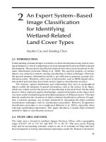
Figure 9.1. By grouping cell applications appropriately, we built a spatially distrib-
uted accounting of moisture in several layers (zones), the distributed large basin run-
off model (DLBRM). Daily precipitation, air temperature, and insolation (the latter
available from cloud cover and meteorological summaries as a function of location
and time of the year) may be used to determine snowpack accumulations, snowmelt
(degree-day computations), and supply, s, into the upper soil zone. Water ow, u, also
enters from upstream cells’ upper soil zones. The total supply is divided into sur-
Supply, s
α
g
G
(s+u)
U
C
Snow Pack

Melt, m Runoff
Snow Rain
Insolation
Precipitation
Temperature
Evapotranspiration, β
ℓ
e
p
L
Upstream, ℓ
Downstream, α
ℓ
L
Evapotranspiration, β
u
e
p
U
Upstream, u
Downstream, α
u
U
Evapotranspiration, β
g
e
p
G
Upstream, g
Downstream, α

w
G
Evaporation, β
s
e
p
S
Upstream, h
Downstream, α
s
S
Surface
Runoff
Interflow
Ground
Water
Percolation, α
p
U
Deep Percolation, α
d
L
Upper Soil
Moisture, U
Lower Soil
Moisture, L
Groundwater
Moisture, G
Surface
Moisture, S

α
i
L
FIGURE 9.1 Model schematic for one cell.
64142.indb 102 11/12/07 9:59:06 AM
© 2008 by Taylor & Francis Group, LLC
Spatially Distributed Watershed Model of Water and Materials Runoff 103
face runoff,
s u U C+
( )
, and inltration to the upper soil zone,
s u U C+
( )
−
( )
1
,
in relation to the upper soil zone moisture content, U, and the fraction it represents
of the upper soil zone capacity, C (variable area inltration). Percolation to the lower
soil zone, a
p
U, evapotranspiration, b
u
e
p
U, and lateral ow to a downstream upper
soil zone, a
u
U, are taken as outows from a linear reservoir (ow is proportional
to storage). Likewise, water ow, ,, enters the lower soil zone from upstream cells’

lower soil zones. Interow from the lower soil zone to the surface, a
i
L, evapotrans-
piration, b
,
e
p
L, deep percolation to the groundwater zone, a
d
L, and lateral ow to
a downstream lower soil zone, a
,
L, are linearly proportional to the lower soil zone
moisture content, L. Water ow, g, enters the groundwater zone from upstream cells’
groundwater zones. Groundwater ow, a
g
G, evapotranspiration from the ground-
water zone, b
g
e
p
G, and lateral ow to a downstream groundwater zone, a
w
G, are
linearly proportional to the groundwater zone moisture content, G. Finally, water
ow, h, enters the surface zone from upstream cells’ surface zones. Evaporation from
the surface storage, b
s
e
p

S, and lateral ow to a downstream surface zone, a
s
S, are
linearly proportional to the surface zone moisture, S. Additionally, evaporation and
evapotranspiration are dependent on potential evapotranspiration, e
p
, as determined
independently from a heat balance over the watershed, appropriate for small areas.
The alpha coefcients (a) represent linear reservoir proportionality factors and the
beta coefcients (b) represent partial linear reservoir coefcients associated with

d
dt
U s u s u
U
C
U U e U
p u u p
= + − +
( )
− − −α α β
(9.1)

d
dt
L U L L L e L
p i d p
= − − − + −α α α α β
, ,
,

(9.2)

d
dt
G L G G g e G
d g w g p
= − − + −α α α β
(9.3)

d
dt
S s u
U
C
L G S h e S
i g s s p
= +
( )
+ + − + −α α α β
(9.4)
Solution
Consideration of equations (9.1)–(9.4) reveals multiple analytical solutions; while
tractable, a simpler approach uses a numerical solution based on nite difference
approximations of equations (9.1)–(9.4). Consider equation (9.1) approximated with
nite differences,

∆ ∆ ∆U s u t
s u
C
e U t

p u u p
≅ +
( )
−
+
( )
+ + +






α α β
(9.5)
64142.indb 103 11/12/07 9:59:10 AM
evapotranspiration. From Figure 9.1,
© 2008 by Taylor & Francis Group, LLC
104 Wetland and Water Resource Modeling and Assessment
where ΔU = change in upper soil zone moisture storage over time interval Δt,
s
,
u
,
and
e
p
= average supply, upstream inow, and potential evapotranspiration rates,
respectively, over time interval Δt, and
U

= average upper soil zone moisture storage
over time interval Δt. By taking ΔU = U – U
0
(where U
0
and U are beginning-of- and
end-of-time-interval storages, respectively) and
U U≅
, equation (9.5) becomes

U
U s u t
s u
C
e t
p u u p
≅
+ +
( )
+
+
+ + +






0
1

∆
∆α α β
(9.6)
Equation (9.6) is good for small Δt and as
∆t → 0
, equation (9.6) approaches the
true solution (converges) to equation (9.1). Likewise, using similarly dened terms,
equations (9.2)–(9.4) become

L
L U t
e t
p
i d p
≅
+ +
( )
+ + + +
( )
0
1
α
α α α β

 
∆
∆
(9.7)

G

G L g t
e t
d
g w g p
≅
+ +
( )
+ + +
( )
0
1
α
α α β
∆
∆
(9.8)

S
S
s u
C
U L G h t
e t
i g
s s p
≅
+
+
+ + +







+ +
( )
0
1
α α
α β
∆
∆
(9.9)
As equations (9.6)–(9.9) are used over time interval Δt, end-of-time-interval values
are computed from beginning-of-time-interval values (e.g., U from U
0
). These end-
of-time-interval values for one time interval become beginning-of-time-interval val-
ues for the subsequent time interval.
Each cell’s inow hydrographs must be known before its outow hydrograph
can be modeled; therefore we arranged calculations in a ow network to assure this.
It is determined automatically from a watershed map of cell ow directions. The
ow network is implemented to minimize the number of pending hydrographs in
computer storage and the time required for them to be in computer storage. We used
the same network for surface, upper soil, lower soil, and groundwater storages. We
implemented routing network computations as a recursive routine to compute out-
ow, which calls itself to compute inows (which are upstream outows) (Croley and
He 2005, 2006).
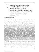
9.3.1 APPLICATION

We have discretized 18 watersheds to date. The elevation map for the Kalamazoo
tions taken from a 30-m digital elevation model (DEM) available from the United
64142.indb 104 11/12/07 9:59:15 AM
River watershed in southwestern Michigan is shown in Figure 9.2. We used eleva-
© 2008 by Taylor & Francis Group, LLC
Spatially Distributed Watershed Model of Water and Materials Runoff 105
States Geological Survey (USGS). We also used USGS land cover characteristics
and the U.S. Department of Agriculture State Soil Geographic Database to add land
cover, upper and lower soil zone parameters (depth, actual water content, and perme-
we used gradient search techniques to minimize root mean square error between
modeled and actual basin outow by selecting the best spatial averages for each
of the eleven parameters; the spatial variation of each parameter follows a selected
watershed characteristic, as shown here and arrived at by experimentation.

α α
p
i
p i
U
f K
( )
= ( , %)80
(9.10)

β β
u
i
u i
U
f K

( )
= ( , %)80
(9.11)

α α
i
i
i i
L
f K
( )
= ( , %)80
(9.12)

α α
d
i
d i
L
f K
( )
= ( , %)80
(9.13)

β β
 
( )
=
i
i

L
f K( , %)80
(9.14)

α α
g
i
g i
L
f K
( )
= ( , %)80
(9.15)

α α
η
s
i
s
i
i
f
s
( )
=







, %80
(9.16)

α α
u
i
u i
U
f K
( )
= ( , %)80
(9.17)

α α
 
( )
=
i
i
L
f K( , %)80
(9.18)

α α
w
i
w i
L
f K

( )
= ( , %)80
(9.19)
Saugatuck,
Michigan, USA
86° 13´ W. Lon.
42° 40´ N. Lat.
612 km east-west
332 km north-south
N
180.00 360.00
FIGURE 9.2 Kalamazoo watershed elevations (m).
64142.indb 105 11/12/07 9:59:20 AM
ability), soil texture, and surface roughness; see Croley et al. (2005). In application,
© 2008 by Taylor & Francis Group, LLC
106 Wetland and Water Resource Modeling and Assessment

C C f C
i
i
U
( )
= ( , %)80
(9.20)

f x
x
n
x
i

i
j
j
n
( , )
%
ε
ε
= −










+
=
∑
1
1
100
1
1
(9.21)
where
α

•
( )
i
= linear reservoir coefcient for cell i,
α
•
= spatial average value of the
linear reservoir coefcient (from parameter calibration),
β
•
( )
i
and
β
•
are dened
similarly for partial linear reservoir coefcients (used in evapotranspiration),
C
i
( )

and
C
are dened similarly for the upper soil zone capacity,
K
i
U
= upper and
K
i

L
=
lower soil zone permeability in cell i, s
i
= slope of cell i,
η
i
= Manning’s roughness
coefcient for cell i,
C
i
U
= upper soil zone available water capacity, x
i
= data value
for cell i, and n = number of cells in the watershed.
Note two parameters not shown here, which govern the heat balance used for snow-
melt and potential evapotranspiration, are taken as spatially constant over the water-
shed. Also, the partial linear reservoir coefcients for the groundwater and surface
zones are taken as zero, ignoring evapotranspiration from those two zones. Thus
there are 13 parameters (of a possible 15) searched in the calibration. To speed up
calibrations, we preprocessed all meteorology for all watershed cells and preloaded
it into computer memory. The correlation between modeled and observed watershed
outows was 0.88, the root mean square error was 0.19 mm/d (compare with a mean
ow of 0.78 mm/d); the ratio of modeled to actual mean ow was 1.00, and the
ratio of modeled to actual ow standard deviation was 0.87 (Croley and He 2006).
We used the model to look at modeling alternatives, including alternative evapo-
transpiration calculations, spatial parameter patterns, and solar insolation estimates.
We also explored scaling effects in using lumped parameter model calibrations to
calculate initial distributed model parameter values (Croley and He 2005; Croley et

al. 2005).
9.3.2 TESTING
As a test of equations (9.6)–(9.9), we used them for Δt = 1.5 minutes to approxi-
mate the solution of equations (9.1)–(9.4) over about 17 years of daily values for
the Maumee River watershed (Croley and He 2006) and found them identical (in
all variables) through three signicant digits (all that were inspected) with the
exact analytical solution. For Δt = 15 minutes, the solution was nearly identical
with only an occasional difference of one in the third signicant digit. As the Mau-
mee River watershed has a very “ashy” response to precipitation (very fast upper
soil and surface storage zones) these comparisons are deemed signicant and the
time intervals should be more than adequate for the slower response of lower soil
and groundwater zones (the Maumee application has no lower soil or groundwater
zones).
64142.indb 106 11/12/07 9:59:25 AM
© 2008 by Taylor & Francis Group, LLC
Spatially Distributed Watershed Model of Water and Materials Runoff 107
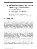
9.4 MATERIALS RUNOFF MODEL
Consider now the addition of some material or pollutant dissolved in, or carried by,
Figure 9.3. At any time, let the concentration of this conservative pollutant in the
inow u be c
u
and in the supply s be c
s
. If these ows do not mix together, then the
fraction U/C of each of these ows runs off directly (without even entering the upper
soil zone) and the surface runoff of pollutant is
sc uc U C
s u
+
( )

. If the concentra-
tion in the upper soil zone moisture storage U is c
U
, then the percolating pollutant is
a
p
Uc
U
and the lateral pollutant ow downstream to the next cell’s upper soil zone is
a
u
Uc
U
. Taking pollutant movement with evaporation as zero, mass continuity (of the
pollutant) gives:

d
dt
Uc sc uc sc uc
U
C
Uc Uc
U s u s u p U u U
( )
= + − +
( )
− −α α
(9.22)
or

d
dt
U s u s u
U
C
U U
c c c c c p c u c
= + − +
( )
− −α α
(9.23)
where s
c
= sc
s
, u
c
= uc
u
, and U
c
= Uc
U
.
s
c
U
c
L
c

G
c
S
c
α
i
L
c
α
g
G
c
α
s
S
c
α
p
U
c
α
d
L
c
h
c
u
c
α
u

U
c
α
ℓ
L
c
(s
c
+u
c
)
U
C
α
w
G
c
g
c
ℓ
c
FIGURE 9.3 Distributed “pollutant” ows schematic for a single cell.
64142.indb 107 11/12/07 9:59:27 AM
the water ows in Figure 9.1, except that none is considered to be evaporated; see
© 2008 by Taylor & Francis Group, LLC
108 Wetland and Water Resource Modeling and Assessment
Likewise from Figure 9.3, mass continuity of the pollutant gives:

d
dt

L U L L L
c p c i c d c c c
= − − − +α α α α


(9.24)

d
dt
G L G G g
c d c g c w c c
= − − +α α α
(9.25)

d
dt
S s u
U
C
L G S h
c c c i c g c s c c
= +
( )
+ + − +α α α
(9.26)
where L
c
, G
c
, and S

c
are the amounts of pollutant in the lower soil zone, the ground-
water zone, and surface storage, respectively, and ,
c
, g
c
, and h
c
are the upstream
pollutant ows from the lower soil zone, the groundwater zone, and surface storage,
respectively.
Solution
Similar to the numerical solution of equations (9.1)–(9.4) [(9.6)–(9.9)], the numerical
solution for equations (9.23)–(9.26) becomes

U
U s u t s u
U
C
t
t
c
c c c c c
p u
≅
+ +
( )
− +
( )
+ +

( )
0
1
∆ ∆
∆α α
(9.27)

L
L U t
t
c
c p c c
i d
≅
+ +
( )
+ + +
( )
0
1
α
α α α


∆
∆
(9.28)

G
G L g t

t
c
c d c c
g w
≅
+ +
( )
+ +
( )
0
1
α
α α
∆
∆
(9.29)

S
S
s u
C
U L G h t
t
c
c
c c
i c g c c
s
≅
+

+
+ + +






+
0
1
α α
α
∆
∆
(9.30)
where terms are dened for material ows in a manner similar to that for water
ows. We used the same network for surface, upper soil, lower soil, and groundwater
storage of pollutant as we used for water ows.
9.4.1 INITIAL AND BOUNDARY CONDITIONS
Suppose a pollutant deposit P exists on top of the upper soil zone. Precipitation or
snowmelt on top of this deposit will produce a supply s to the upper soil zone that
64142.indb 108 11/12/07 9:59:31 AM
© 2008 by Taylor & Francis Group, LLC
Spatially Distributed Watershed Model of Water and Materials Runoff 109
will dissolve some of this pollutant, producing a pollutant concentration c
s
. If we
regard this process as independent of other ows to the top of the upper soil zone (u
and u

c
= uc
u
), we can model the pollutant uptake as follows.

d
dt
P sc P
P
s
= − >
= =
,
,
if
if
0
0 0
(9.31)
The nite difference solution is

P P sc t sc t P
sc t P
s s
s
= − <
= ≥
0 0
0
0

∆ ∆
∆
,
,
if
if
(9.32)
where P and P
0
are the end- and beginning-of-time-interval pollutant values,
respectively. The pollutant delivered to the top of the upper soil zone would be
s u sc uc
c c s u
+ = +
as used in equations (9.27) and (9.30).
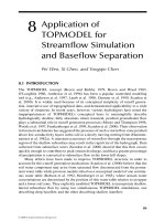
9.5 EXAMPLE SIMULATION
Selected lateral ows simulated by the model for the upper soil zone, groundwater
for the rst two months of 1952. Although the simulation was daily, the ows are
shown weekly in Figure 9.4. The initial conditions for this simulation included 1 cm
of (arbitrary) pollutant on the surface of the watershed on 1 January 1952. Within
two weeks it was gone from the surface (@ c
s
= 1.0 m
3
of pollutant / m
3
of water).
Columns 1 through 3 in Figure 9.4 show that lateral water ows in the watershed
were fairly uniform for the period with perhaps higher surface water ows on 1 and
15 January (more of the streamow network is seen to respond then). Column 4

illustrates that even at the end of day 1, the upper soil zone already had pollutant in
it; uper soil zone (USZ) pollutant ows peaked on 15 January and slowly tapered off
through the end of February. Pollutant did not appear in any sizable manner in the
groundwater zone until the end of February, as illustrated in column 5 of Figure 9.4.
The pollutant ow in the surface network, shown in the last column in Figure 9.4,
responds midway between the USZ and ground water zone (GWZ) responses. There
is a high ush on the rst day, corresponding with the initial condition (placing pol-
lutant on the surface of the watershed at the beginning of day 1) and the increased
surface water ow; the surface pollutant map shows extensive response. The surface
response then drops off as pollutant is only available in the USZ and GWZ. How-
ever, on 15 January, the surface pollutant response increases with the ush of water
through the USZ that occurs then (see third row in columns 3 and 4 in Figure 9.4).
9.6 SUMMARY
Prediction and management of watershed water quality require estimation of non-
point source material movement throughout the watershed. We briey reviewed
64142.indb 109 11/12/07 9:59:33 AM
zone, and surface zone are shown in Figure 9.4 for the Kalamazoo River watershed
© 2008 by Taylor & Francis Group, LLC
110 Wetland and Water Resource Modeling and Assessment
distributed agricultural runoff models and learned that there are no integrated
spatially distributed, physically based watershed-scale hydrological/water quality
models available to evaluate movement of materials in both surface and subsurface
waters. Either the hydrology is limited to very simple empirical descriptions or the
application is made to only very coarse spatial discretizations of the watershed. We
adapted an existing lumped-parameter conceptual water balance model of watershed
hydrology into a spatially distributed model of runoff. It employs moisture storage
in the upper and lower soil zones, in a groundwater zone, and on the surface, with
lateral ows from all storages into similar storages in adjacent grid cells dened over
the watershed. By applying the surface drainage network to all storage lateral ows,
we can trace the movement of water throughout the watershed. We further adapt the

distributed model to incorporate the storage and movement of an arbitrary mate-
rial, conservative in nature, and to trace its movement throughout the watershed. By
0 1(19520101) 0 20(19520101) 0 500(19520101) 0 0.05(19520101) 0 0.5(19520101) 0 10(19520101)
0 1(19520108) 0 20(19520108) 0 500(19520108) 0 0.05(19520108) 0 0.5(19520108) 0 10(19520108)
0 1(19520115) 0 20(19520115) 0 500(19520115) 0 0.05(19520115) 0 0.5(19520115) 0 10(19520115)
0 1(19520122) 0 20(19520122) 0 500(19520122) 0 0.05(19520122) 0 0.5(19520122) 0 10(19520122)
0 1(19520129) 0 20(19520129) 0 500(19520129) 0 0.05(19520129) 0 0.5(19520129) 0 10(19520129)
0 1(19520205) 0 20(19520205) 0 500(19520205) 0 0.05(19520205) 0 0.5(19520205) 0 10(19520205)
0 1(19520212) 0 20(19520212) 0 500(19520212) 0 0.05(19520212) 0 0.5(19520212) 0 10(19520212)
0 1(19520219) 0 20(19520219) 0 500(19520219) 0 0.05(19520219) 0 0.5(19520219) 0 10(19520219)
0 1(19520226) 0 20(19520226) 0 500(19520226) 0 0.05(19520226) 0 0.5(19520226) 0 10(19520226)
USZ
Water Water Water Pollutant Pollutant Pollutant
USZGWZ GWZ SurfaceSurface
FIGURE 9.4 Kalamazoo model lateral ows (cm/d).
64142.indb 110 11/12/07 9:59:34 AM
© 2008 by Taylor & Francis Group, LLC
Spatially Distributed Watershed Model of Water and Materials Runoff 111
employing a numerical solution instead of the analytical solution used in the original
lumped-parameter water balance model, we are able to easily represent the mass
balance of both water and an arbitrary conservative pollutant spatially throughout
all storage zones in the watershed. Model testing reveals that the numerical solu-
tion converges to the analytical solution for a 1-km
2
grid on a watershed with a
very fast response. By assigning initial pollutant surface amounts and introducing a
single parameter (pollutant concentration in water), we can model its movement. In
a simple example on the Kalamazoo River watershed, in which a uniform layer of
pollutant is assumed initially, we present the consecutive spatial distributions that
occur over a two-month simulation, demonstrating that the model could be used to

simulate real-world material movement in a watershed.
ACKNOWLEDGMENTS
This is GLERL Contribution No. 1375.
REFERENCES
Arnold, G., R. Srinavasan, R. S. Muttiah, and J. R. Williams. 1998. Large area hydrologic
modeling and assessment. Part I: Model development. Journal of the American Water
Resources Association 34: 73–89.
Beasley, D. B., and L. F. Huggins. 1980. ANSWERS (Areal Nonpoint Source Watershed Envi-
ronment Simulation): User’s manual. West Lafayette, IN: Department of Agricultural
Engineering, Purdue University.
Beven, K. J. 2000. Rainfall-runoff modeling: The primer. New York: John Wiley & Sons.
Bicknell, B. R., J. C. Imhoff, J. Kittle, A. S. Donigian, and R. C. Johansen. 1996. Hydrologi-
cal Simulation Program—FORTRAN, user’s manual for release 11. Athens, GA: U.S.
Environmental Protection Agency, Environmental Research Laboratory.
Crawford, N. H., and R. K. Linsley. 1966. Digital simulation in hydrology: Stanford water-
shed model IV. Technical Report 39. Stanford, CA: Department of Civil Engineering,
Stanford University.
Croley, T. E. II., 2002. Large basin runoff model. In Mathematical models of large water-
shed hydrology, ed. V. Singh, D. Frevert, and S. Meyer. Littleton, CO: Water Resources
Publications, 717–770.
Croley, T. E., II, and C. He. 2005, Distributed-parameter large basin runoff model I: Model
development. Journal of Hydrologic Engineering 10: 173–181.
Croley, T. E., II, and C. He. 2006. Watershed surface and subsurface spatial intraows. Jour-
nal of Hydrologic Engineering 11(1):12–20.
Croley, T. E., II, C. He, and D. H. Lee. 2005. Distributed-parameter large basin runoff model
II: Application. Journal of Hydrologic Engineering 10: 182–191.
Garen, D. C., and D. S. Moore. 2005. Curve number hydrology in water quality modeling:
uses, abuses, and future directions. Journal of the American Water Resources Associa-
tion 41: 377–388.
Ghadiri, H., and C. W. Rose. 1992, Modeling chemical transport in soils: Natural and applied

contaminants. Ann Arbor, MI: Lewis Publishers.
Kawkins, R. H. 1978. Runoff curve number relationships with varying site moisture. Journal
of the Irrigation and Drainage Division 104: 389–398.
Knisel, W. G. 1980. CREAMS: A eldscale model for chemical, runoff, and erosion from
agricultural management systems, Conservation Report No. 26. Washington, DC: U.S.
Department of Agriculture, Science and Education Administration.
64142.indb 111 11/12/07 9:59:34 AM
© 2008 by Taylor & Francis Group, LLC
112 Wetland and Water Resource Modeling and Assessment
Lahlou, N., L. Shoemaker, S. Choudhury, R. Elmer, A. Hu, H. Manguerra, and A. Parker.
1998. BASINS V.2.0 user’s manual. Washington, DC: U.S. Environmental Protection
Agency Ofce of Water, EPA-823-B-98-006.
Leonard, R. A., W. G. Knisel, and D. A. Still. 1987. GLEAMS: Groundwater loading effects
of agricultural management systems. Transactions of ASAE 30:1403–1418.
Sharpley, A. N., and J. R. Williams. 1990. EPIC—erosion/productivity impact calculator,
Technical Bulletin No. 1768. Washington, DC: U.S. Department of Agriculture, Agri-
cultural Research Service.
U.S. Environmental Protection Agency. 2002. National water quality inventory 2000 report.
EPA-841-R-02-001. Washington, DC: U.S. Environmental Protection Agency.
Wischmeier, W. H., and D. D. Smith. 1978. Predicting rainfall erosion losses. Agricultural
Handbook No. 537. Washington, DC: U.S. Department of Agriculture.
Young, R. A., C. A. Onstad, D. D. Bosch, and W. P. Anderson. 1989. AGNPS: A nonpoint-
source pollution model for evaluating agricultural watersheds. Journal of Soil and
Water Conservation 44:168–173.
64142.indb 112 11/12/07 9:59:34 AM
© 2008 by Taylor & Francis Group, LLC