WETLAND AND WATER RESOURCE MODELING AND ASSESSMENT: A Watershed Perspective - Chapter 13 potx

Part IV
Wetland Biology and Ecology
© 2008 by Taylor & Francis Group, LLC
153
13
Soil Erosion Assessment
Using Universal Soil Loss
Equation (USLE) and
Spatial Technologies—
ACaseStudyatXiushui
Watershed, China
Hui Li, Xiaoling Chen, Liqiao Tian,
and Zhongyi Wu
13.1 INTRODUCTION
Accelerated soil erosion is one of the most serious environmental problems in the
world. In China, millions of tons of topsoil are eroded and transported every year,
which not only degrades soil resources but also causes detrimental environmental
consequences. Soil erosion affects productivity by changing soil properties, and par-
ticularly by destroying topsoil structure, reducing soil volume and water holding
capacity, reducing inltration, increasing runoff and washing away nutrients such
as nitrogen, phosphorus, and organic matter (Meyer et al. 1985; Oyedele 1996). The
resulting sediments act as carriers of pollutants including heavy metals, pesticides,
and others.
Jiangxi is a province that suffers severely from soil erosion. The total affected
area is 336.12 × l0
4
ha, which accounts for 95.5% of the total provincial area, and is
mainly distributed in the upper and middle valley of the Xiu River, Ganjiang River,
Xin River, Fu River, and around Poyang Lake.
The Xiushui watershed discharges water and sediments into Poyang Lake, which
is the largest freshwater lake in China and an important international wetland with

considerable ecosystem functions. Regional economic development, deforestation,
and soil erosion in the Xiushui watershed have degraded the wetland ecological
environment of Poyang Lake. Before effective management measures can be taken,
the amount and location of soil that has been eroded must be quantied.
There are many models available for erosion estimation. Some of these models
are based on physical parameters such as the WEPP (Water Erosion Prediction Proj-
ect), and some are empirically orientated, such as the universal soil loss equation
© 2008 by Taylor & Francis Group, LLC
154 Wetland and Water Resource Modeling and Assessment
(USLE). However, modeling soil erosion is difcult because of the complexity of
the interactions of factors that inuence the erosion (Wischmeier and Smith 1978).
The objective of this paper is to estimate soil erosion and prioritize watersheds with
respect to the intensity of soil erosion using the USLE.
13.2 STUDY AREA
Niushui Watershed
N
Xiushui Xian
Wuning Xian
Yongxiu Xian
Anvi Xian
Jing’ an Xian
Tonggu Xian
0
20 40
60
80
KM
Legend
River
Country

Fengxin Xian
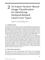
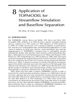
FIGURE 13.1 Location of Xiushui watershed.
© 2008 by Taylor & Francis Group, LLC
Xiushui watershed is a subset of the Poyang Lake watershed in Jiangxi Province
(Figure 13.1). It covers 14,606 km
2
and is located between 28° 22′ 29″ to 29° 32′ 18″
north latitude and 114° 3′ 15″ to 115° 55′ 32″ east longitude. Most of the watershed is
mountainous area ranging from about 1 m to 1772 m above sea level with an average
elevation of 341 m above sea level. The Xiu River runs from the southwest to the east
and then discharges into Poyang Lake. The watershed is characterized by a fragile
Soil Erosion Assessment Using Universal Soil Loss Equation (USLE) 155
ecosystem with frequent oods and relatively lagged development compared with its
neighborhood, due to its unique geographic characteristics.
The watershed is situated in a subtropical zone with a monsoonal climate. The
annual average temperature is 17°C. Annual precipitation averages 1613.7 mm, of
which 73.1% occurs between March and August. The dominant agricultural crops
are rice, cotton, and tea. The major soil types consist of red soil, brown soil, yel-
low-brown soil, weakly developed red soil, yellow soil, and paddy soil. The land is
partially cultivated while the rest is covered with vegetation.
13.3 METHODS
The overall methodology involves using a soil erosion model, USLE, in a GIS (geo-
graphic information system) that incorporates data derived from remote sensing
imagery, statistical data obtained from weather stations, and information from soil
surveys. Individual raster data layers were built for each factor in USLE and pro-
cessed by cell-grid modeling procedures in GIS to account for the spatial variability
across the domain. With a consideration of the resolutions of all source data and the
study site, the grid cells were set to 100 × 100 square meters.
13.3.1 GOVERNING EQUATION
The USLE was hailed as one of the most signicant developments in soil and water

conservation in the twentieth century. It is an empirical technology that has been
applied around the world to estimate soil erosion by raindrop impact and surface
runoff. The USLE provides a quick approach to estimating long-term average annual
soil loss. The model was originally developed and widely applied for a plane area.
However, studies in mountainous areas have been conducted as well, and the results
veried its ability to model complex landscapes (Bancy et al. 2000, Lufafa et al.
2003). It is expressed as follows:
(13.1)
where A is annual soil loss (t ha
−1
yr
−1
); R is the rainfall erosivity factor; K is the soil
erodibility factor; L is the slope length factor; S is the slope steepness factor; C is the
crop and management factor; and P is the conservation supporting practices factor.
L, S, C, and P are dimensionless.
13.3.2 DETERMINING THE USLE FACTOR VALUES
13.3.2.1 Rainfall Erosivity (R) Factor
The R factor represents the rainfall and runoff’s impact on soil. Originally, it was
calculated as the total kinetic energy of the storm and its maximum 30-minute inten-
sity (I30). Frequently, however, there are not enough data available to compute the R
value using this method, especially for a large area. Different replacement methods
have been developed over time for the computation of R. An erosivity index for river
© 2008 by Taylor & Francis Group, LLC
A R K L S C P= ⋅ ⋅ ⋅ ⋅ ⋅

156 Wetland and Water Resource Modeling and Assessment
basins, developed by Fournier (1960), was subsequently modied by the FAO (Food
and Agriculture Organization of the United Nations) as follows:
(13.2)

where r
i
is the rainfall per month and P is the annual rainfall. This index is summed
for the whole year and found to be linearly correlated with the EI30 index (R) of the
USLE as follows:
(13.3)
where a and b are the constants that need to be determined and vary widely among
different climatic zones. You and Li (1999) presented the values of a and b for Taihe
County, Jiangxi province, which is only one hundred kilometers away from the study
area.
According to his study, a and b are 4.17 and −152, respectively. The unit of R was
then converted into MJ mm ha
−2
h
−1
. Due to the large area of the watershed, data
from seven meteorological stations were chosen to calculate the precipitation of the
entire watershed. Among the seven stations, one is situated within the watershed,
and the other six are in the neighborhood of the study area. Monthly rainfall data of
seven stations over a time span from 1971 to 2000 were collected from the national
meteorological bureau. The R value was calculated based on each of the seven sta-
tions by using the aforementioned method, and then interpolated into a continuous
surface in GIS.
13.3.2.2 Soil Erodibility (K) Factor
The K factor measures soil susceptibility to rill and inter-rill erosion. Various meth-
ods for computing the K value were developed by researchers. As for this study, the
detailed soil properties such as silt, sand, clay, and organic matter content could be
acquired from the results of China’s second soil survey. Liang et al. (1999) studied
the area’s soil erodibility and presented the K factor values corresponding to differ-
ent soil types. In this study, we adopted their results for the estimation.

13.3.2.3 TopographicFactor(LS)
Slope length and slope gradient have substantial effects on soil erosion by water.
The two effects are represented in the USLE by the slope length factor (L) and the
slope steepness factor (S). L and S are best determined by pacing or measuring in the
eld, but extensive eldwork is both time consuming and labor extensive. A digital
elevation model (DEM) is a useful source for describing the topography of the land
surface and is employed in LS calculation. There are some problems found in LS
estimation by traditional methods, which assume that the length factor is dened as
the distance to the divide or upslope border of the eld. However, two-dimensional
overland ow and the resulting soil loss actually depend on the area per unit of con-
tour length contributing runoff to that point. The latter may differ considerably from
© 2008 by Taylor & Francis Group, LLC
F r P
i
i
=
=
∑
2
1
12
/

R a F b= ⋅ +

Soil Erosion Assessment Using Universal Soil Loss Equation (USLE) 157
the manually measured slope length, as it is strongly affected by ow convergence
and/or divergence (Desmet and Govers 1996). The new concept was forwarded and
some software such as Usle2D (Desmet and Govers 2000) was designed to overcome
this problem by replacing the slope length by the unit contributing area.

13.3.2.4 Crop and Management Factor (C)
The C factor in the USLE measures the combined effect of the interrelated cover and
crop management variables (Folly et al. 1996). The C factor could be evaluated from
long-term experiments where soil loss is measured from land under various crops
and crop management practices. However, such experimental installations are rarely
available for a wide range of areas. Remote sensing provides a powerful tool for
the observation and study of landscapes. Vegetation indices (VI) are robust spectral
measures of the amount of vegetation present on the ground. They typically involve
transformations of spectral information to enhance the vegetation signal and allow
for precise intercomparisons of spatiotemporal variations in terrestrial photosyn-
thetic activity (United States Geological Survey [USGS] 2004). Vegetation indices
(VI) are widely used to measure the amount, structure, and condition of vegetation.
Evidence indicates that there is a relationship between the VI and C factor (Tweddale
et al. 2000). With this in mind, we could develop a more efcient method for C factor
estimation. Ma (2003) and Cai et al. (2000) presented the relationship between veg-
etation cover and NDVI (Normalized Distance Vegetation Index), vegetation cover
and C factor, respectively. They are expressed as follows:
where C is the C factor in the USLE. MODIS Level 3 series products cover NDVI,
and the USGS NDVI data used in this study was compiled based on the images
obtained from June 1 to 15, 2004.
13.3.2.5 Erosion Control Practice Factor (P)
The erosion control practice factor (P factor) is dened as the ratio of soil loss with
a given surface condition to soil loss with up-and-downhill plowing. The P factor
accounts for the erosion control effectiveness of such land treatments as contouring,
compacting, establishing sediment basins, and other control structures (Angimaa et al.
2003). However, most of the study areas are mountains covered with forest, and there
is no signicant conservation practice installed. In this study, P was assumed to be 1.
© 2008 by Taylor & Francis Group, LLC

V I

c c
= +108 49 0 717. .

R
2
0 77= .

(13.4)
where V
c
is vegetation cover (%) and I
c
is the NDVI.
The following is the relationship between C factor and vegetation cover:

C V
C V V
C V
c
c c
c
= ≤
= − < ≤
= ≥
1 0
0 658 0 3436 0 78 3
0 78
. . lg . %
%3






(13.5)
158 Wetland and Water Resource Modeling and Assessment
13.4 RESULTS AND DISCUSSION
13.4.1 F
ACTORS IN USLE
The monthly average rainfall and the calculated rainfall erosivity are listed in
Table 13.1, which shows that most of the precipitation was concentrated in May,
June, and July. This result suggests that most of the erosion might occur within the
rainfall season and can be largely ascribed to major storms.
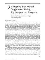
The rainfall erosivity ranges from 5,733.4 to 12,628 and the highest erosivity was
observed in Lushan, which is situated just northeast of the watershed. The nearby
Jiujiang station has an erosivity of only 5,733.4 for the lower elevation with less
rainfall compared to Lushan. Nanchang, the northernmost station with the most ade-
quate rainfall, has an erosivity of 9,284.1. Jian, whose station is latitudinally located
between Xiushui and Nanchang, has less rainfall erosivity compared to Nanchang.
The general rainfall erosivity is shown in Figure 13.2.
TABLE 13.1
Monthly average of rainfall and rainfall runoff erosivity
for each meteorological station.
a
Station Jan Feb Mar Apr May Jun Jul Aug Sep Oct Nov Dec Erosivity
Xiushui 70.2 93.6 147.9 222.9 215.4 299.4 177.9 116.7 84.6 78.9 63.6 42.6 8520.8
Lushan 75.9 99.6 157.5 224.1 258.0 315.9 249.9 289.2 149.1 115.5 85.5 48.0 12628
Nangchang 74.1 100.8 175.5 223.8 243.9 306.6 144.0 129.0 68.7 59.7 56.7 41.4 9284.1
Pingjiang 72.9 89.4 146.1 198.0 214.2 251.7 174.3 134.7 73.2 76.8 60.9 39.9 7162
Jian 73.4 103.2 169.0 224.4 214.6 234.0 116.3 134.5 79.6 74.2 55.0 40.7 7041.8

Jiujiang 51.8 95.0 137.0 183.6 193.1 213.7 141.0 131.8 95.5 96.5 64.8 40.3 5733.4
Jiayu 58.5 73.2 124.5 166.3 188.3 244.8 163.0 123.6 75.1 95.7 64.4 36.8 6017.3
a
Units for rainfall and erosivity are mm and MJ mm hm
−2
h
−1
, respectively.
FIGURE 13.2 Map of rainfall erosivity. (See color insert after p. 162.)
© 2008 by Taylor & Francis Group, LLC
K Value Map
5733.4 12628
Soil Erosion Assessment Using Universal Soil Loss Equation (USLE) 159
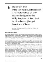
The K factor value for each soil type was obtained from previous studies done
in the area. The K factor map was thus prepared by assigning the K value to each
soil type in a soil map. The values are given in Table 13.2 and the map shown in
Figure 13.3. The erodibility of soils in this area varied from 0.12 for brown soil to
0.413 for moisture paddy soil. As shown in the K value map (Figure 13.3), the most
easily erodible soil is only distributed in the easternmost portion of the watershed
and covers a very small area. The soil with the biggest erosion is in the middle and
eastern part of the study area and did not account for the larger area as well. The rest
of the watershed is occupied by soils with relatively moderate erodibility.
The LS factor was calculated from the DEM for the entire watershed (Figure 13.4).
The statistics demonstrate the variation of LS values (Table 13.3). We can determine
from the LS map that the low LS value (at area) is distributed along the valleys of the
Xiushui River and its tributaries. The high LS value is in the mountainous area with
steep slopes, which may result in higher amounts of erosion. The LS value ranges
from 0 in very at valleys to more than 300 in steep mountains. As to the distribution
of LS values, 37.31% of the area is under 10, which indicates that the region is not
topographically prone to erosion. LS values between 10 and 50 account for 37.51%

of the watershed. The rest exhibit high LS values of more than 50 and extremely
high values of more than 300, which cover 24.86% and 0.33%, respectively, and will
surely result in severe erosion if no conservation practices are installed. Such large
K Value Map
0.0158 0.0544
FIGURE 13.3 Map of soil erodiblility. (See color insert after p. 162.)
TABLE 13.2
K values for major soils.
a
Soil
Red
earth
Brown
earths
Yellow-
brown
earths
Weakly
developed
red earths
Yellow
earths
Moisture
paddy
K value 0.0304 0.0158 0.0288 0.0299 0.0252 0.0544
a
Units for soil erodibility is MghMJ
−1
mm
−1

.
© 2008 by Taylor & Francis Group, LLC
160 Wetland and Water Resource Modeling and Assessment
variation of LS values can be ascribed to the complex mountainous landforms of the
area, which is very typical in the erosion-stricken areas of southern China.
A map of cover and management factors is shown in Figure 13.5. It could be gen-
erally concluded that most of the watershed area is well covered with dense vegetation
except certain sites in the northern and southern mountains whose severe deforesta-
tion would result in a very high C value and thus might lead to serious erosion.
In this study, a grid cell size (of all raster layers) was set to 100 × 100 m. However,
the original resolution of the DEM is 93 × 93 m, and MODIS NDVI’s is 250 × 250 m.
The nearest neighborhood resample method was used to transform the raster layers
into the desired resolution with an accuracy of less than one pixel. Given the same
resolutions, the raster layers could be conducted using GIS overlay procedures.
The resolution will affect the accuracy of the result. The ner the resolution,
the better the accuracy yields and vice versa. However, the ne resolution increases
the amount of data, which results in longer processing time and the need for greater
storage capacity. It is usually suitable for detailed analysis in small geographic areas.
The coarse resolution has no such problems but it leads to larger errors. Taking both
study area and input efforts into consideration, we identied the resolution to be 100
× 100 m, which was found to be appropriate and effective.
LS Value Map
0 >435
FIGURE 13.4 Map of topography. (See color insert after p. 162.)
TABLE 13.3
LS distribution for the watershed.
LS Cell counts Percent (%) LS Cell counts Percent (%)
0–10 546781 37.31% 50–100 252131 17.20%
10–20 181687 12.40% 100–200 98130 6.70%
20–30 146752 10.01% 200–300 14025 0.96%

30–50 221265 15.10% >300 4849 0.33%
© 2008 by Taylor & Francis Group, LLC
© 2008 by Taylor & Francis Group, LLC
Soil Erosion Assessment Using Universal Soil Loss Equation (USLE) 161
13.4.2  erosion intensity
After the factor values were assigned or calculated for each of the grid cells, the
factor maps were overlaid to produce a visualization of soil erosion estimation
(Figure 13.6). The map indicates that the whole area is generally at very low risk
for erosion.
Some statistical results showed that annual average soil losses for the watershed
were 14.36 tons/ha and the standard deviation was 27.28 tons/ha, which suggests that
the variation among estimations for the entire watershed was rather small. However,
some extremely high estimations of more than 500 tons/ha occur in certain places,
which is in accord with the current situation as mentioned in the introduction section
of this paper. Measures, such as constructing terraces, strip cropping and returning
eld to forest should be taken to prevent further soil erosion.
The estimation was further prioritized into six classes: very slight, slight, mod-
erate, severe, very severe, and extremely severe, according to the soil erosion clas-
C Value Map
0 0.001 1.0
FIgure 13.5 
0 0.001 >500
t/ha
Estimation of erosion
FIgure 13.6  Map of erosion intensity. (See color insert after p. 162.)
Map of cover and management. (See color insert after p. 162.)
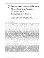
sication criterion of China (Figure 13.7). From Figure 13.7, we can conclude that
162 Wetland and Water Resource Modeling and Assessment
89.14% of the watershed is under the tolerable erosion amount (5 tons/ha); 10.86%
of the study area undergoes erosion, among which only 0.7% and 0.21% suffer from

very and extremely severe erosion, respectively. Some very high estimates were
observed in mountainous places with bad deforestation and could be distributed into
the high LS and C values for these places. The rest of the watershed is relatively less
affected by erosion.
As seen in the maps, the estimated erosion is very sensitive to the LS and C fac-
tors. The patterns in LS and C value maps are very similar to those of the erosion
map, which may illustrate again that the soil conservation measures should be aimed
at decreasing slope with less length and providing better cover to protect soil from
rainfall and runoff detachment.
This method is not veried by real data for there is no measured data avail-
able. However, a four-day intensive eld measurement effort was made in early July
2005 in order to collect ground truth information for erosion intensity. Thirty-three
sites were checked and the vegetation cover and slope were investigated to estimate
the erosion level. According to the eld analysis, the estimations of this method
generally reected the erosion conditions of this watershed. Further investigations
were made to explain the most likely reasons for the erosion, which could be sum-
marized as follows: the construction new roads, the construction of quarries, the
chopping of the forest for fuel or wood, and forest res. All of the activities result in
poor vegetation cover, thus exposing the soil directly to raindrop splash and runoff
detachment.
13.5 CONCLUSIONS
In general, it is clear from the results of this study that USLE is an effective model
for the qualitative as well as quantitative assessments of soil erosion intensity for the
purposes of conservation management. Remote sensing imaging has provided valu-
able data sources, and the MODIS Level 3 VI products provide robust vegetation
measurements for derivation of the C factor in this study. It is difcult to estimate the
0-5 5-25 25-50 50-80 80-150 >150
Erosion estimation (ton/ha/y)
89.14%
7.50%

1.67%
0.79%
0.70%
0.21%
Area (km
2
)
14000
12000
10000
8000
6000
4000
2000
0
FIGURE 13.7 Histogram of erosion estimation.
© 2008 by Taylor & Francis Group, LLC
FIGURE 2.3
FIGURE 2.4
FIGURE 2.5
© 2008 by Taylor & Francis Group, LLC
FIGURE 3.1
FIGURE 3.3
© 2008 by Taylor & Francis Group, LLC

FIGURE 4.6 FIGURE 4.7
© 2008 by Taylor & Francis Group, LLC

FIGURE 4.9 FIGURE 4.11
© 2008 by Taylor & Francis Group, LLC

FIGURE 7.1
FIGURE 7.5
© 2008 by Taylor & Francis Group, LLC
FIGURE 7.6
FIGURE 10.2
© 2008 by Taylor & Francis Group, LLC
FIGURE 12.1
© 2008 by Taylor & Francis Group, LLC
FIGURE 13.2

FIGURE 13.3 FIGURE 13.4

FIGURE 13.5 FIGURE 13.6
© 2008 by Taylor & Francis Group, LLC
FIGURE 16.1
FIGURE 16.6
© 2008 by Taylor & Francis Group, LLC
FIGURE 17.2
FIGURE 17.7
© 2008 by Taylor & Francis Group, LLC
FIGURE 17.4
© 2008 by Taylor & Francis Group, LLC
FIGURE 18.6
© 2008 by Taylor & Francis Group, LLC
FIGURE 18.7
FIGURE 18.8
© 2008 by Taylor & Francis Group, LLC
FIGURE 20.4
© 2008 by Taylor & Francis Group, LLC