Heavy Metals in the Environment: Using Wetlands for Their Removal - Chapter 15 (end) pot

169

A

PPENDICES

L1401-frame-A1 Page 169 Monday, April 10, 2000 10:23 AM
© 2000 by CRC Press LLC

171

A

PPENDIX

A1
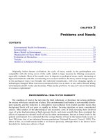
Symbols Used in Systems Diagrams
(a) Producer (b)Consumer
(c) Miscellaneous
Box
(g) Storage
(h) Interaction
(Production)
(i) Switch
(j) Amplifier (l) Exchange
(f) Heat Sink(d) Source
(k) Adding &
Splitting
(e) Defined Boundary
$

L1401-frame-A1 Page 171 Monday, April 10, 2000 10:23 AM
© 2000 by CRC Press LLC

173

A

PPENDIX

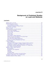
A4
Biogeochemical Cycle of Lead
and the Energy Hierarchy

Howard T. Odum

Table A4.1 Global Storages of Lead
Note Item E10 Grams

1 Seawater recently 2.74 E3
2 Seawater originally 21.9
3 Atmosphere now 1.84
4 Atmosphere originally 0.28
5 Soil, glaciers 4.8 E5
6 Deltas, wetlands, sediments 4.8 E9
7 Land 3.2 E9
8 Ore 1.4 E4
9 Civilization 3.47 E4

Notes:

1, 3, 5, 6. Nriagu (1978, page 10).
2. Use concentration in the deep sea as representative:
0.02

µ

g/kg (from Chow and Patterson, 1966).
(2 E-5 g/m

3

)(1.37 E9 m

3

seawater) = 2.7 E4 g.
4. In original air 5.3 E-10 g/m

3

surface air (from Patter-
son, 1965).
(5.3 E-10 g/m

3

)(1 E-3 m

3

/g surface air)(5.2 E21 g
atmosphere) = 0.28 E10 g.
7. Lead is 16 ppm in rock (Bowen, 1979) 2.2 E24 g.
Uplifted continental sediments: (16 E-6 g/g rock)(2.2
E24 g) = 3.15 E19 g.
8. Lead reserves 141 E6 short tons (Kesler, 1978).
(141 E6)(0.907) = 128 E6 tonne = 1.28 E14 g.
9. Civilization storage, order of magnitude estimate: Net
production rate in Figure 4.6 (4000–534 E9
g/year)(100 years) = 3.47 E14 g.

L1401-frame-A4 Page 173 Monday, April 10, 2000 10:25 AM
© 2000 by CRC Press LLC

174 HEAVY METALS IN THE ENVIRONMENT: USING WETLANDS FOR THEIR REMOVAL

Table A4.2 Global Flows of Lead in Figure 4.6
Note Item E9 Grams/Year

1 Seawater to sediments 2.5
2 Seawater to atmosphere 2 E-5
3 Atmosphere to seawater 210
4 Atmosphere to ecosystems 320
5 Ecosystems runoff to deltas 720
6 Predevelopment runoff 180
7 Deltas to open seawaters 34
8 Deltas and sediments to deep earth ?
9 Deltas, sediments to land 94
10 Sedimentary land to ecosystems 400

11 Normal weathering to ecosystems 18
12 Deep earth to land ?
13 Continental land to ores ?
14 Ores to economy 4000
15 Deep earth to ores ?
16 Economy to atmosphere 440
17 Economy via rivers to sediments 60
18 Economy solids to land 34
19 Volcanoes to atmosphere 0.4
20 Land to atmosphere 5.9
21 Land dust and organics to atmosphere 32

Notes:

1–5, 8, 10, 12–19, 21. Nriagu (1978).
6. River runoff before wastes: 180 E9 g/year (from Bowen,
1966).
Natural denudation 1.1 E10 g/year (Tatsumoto and Patter-
son, 1963).
7. To open sea 34 E9 g/year (after Tatsumoto and Patterson,
1968 quoted by Chow, 1978).
9. Land cycle: (2.4 cm/1000 year)(2.6 g/cm

3

)(1.5 E18 cm

3

) =

9.36 E15 g/year.
(9.36 E15 g/year)(10 E-6 g lead/g land) = 93.6 E9.
11. 180,000 tons/year from natural weathering of rocks
(Volesky, 1990).
20. Land to atmosphere: 5.9 E9 g/year (Lantzy and Mackenzie,
1979).

L1401-frame-A4 Page 174 Monday, April 10, 2000 10:25 AM
© 2000 by CRC Press LLC

BIOGEOCHEMICAL CYCLE OF LEAD AND THE ENERGY HIERARCHY 175

Table A4.3 Emergy per Mass and Concentration of Lead Graphed in Figure 4.7
Note Item Concentration (g/m3)
Emergy per Mass
(sej/g)

1 Ocean 3 E-5 0
2 Inland cycle 16 1 E9
3 Recycled in wetland 100 1.7 E9
4 Lead core 6.55 E4 4.5 E9
5Refined lead 11.3 E6 7.3 E10

Notes:

g = gram; m

3

= cubic meter; sej = solar emjoules; cm

3

= cubic centimeter.
1. Zero emergy when no further dispersion is possible (no available energy in the
concentration); ocean has lowest lead concentration of the main phases
of the geobiosphere (Garrels, Mackenzie, and Hunt, 1975).
2. Assigned a share of the global emergy contribution to the continental earth cycle
(Kuroda, 1982; Drever et al., 1988). Transformity is that of the land cycle
= (9.44 E24 sej/year)/(9.36 E15 g/year) = 1.0 E9 sej/g.
3. Evaluated from wetland system containing lead (Figure 4.7). Emergy in support,
6.3 E10 sej/m

2

/year from Table 5.4 divided by 0.1 g/m

2

/day from Figure
8.2 times 365 days/year = 1.73 E9 sej/g. See Figure 4.6. Concentration
in wetland = 100 ppm.
4. Assigned a share of the global emergy contribution (9.44 E24 sej/year) to the
earth cycle in maintaining orographic uplift (2.15 E15 g/year). Lead in
ore, 6.55% (Kesler, 1978).
5. Emergy per gram from Pritchard, Appendix A11, Figure A11.7 and Table A11.6;
lead per volume = (11.3 g/cm

3

)(1 E6 cm

3

/m

3

) = 11.3 E6 g/m

3

.

L1401-frame-A4 Page 175 Monday, April 10, 2000 10:25 AM
© 2000 by CRC Press LLC

177

A

PPENDIX

A5

A

Field Measurement Methods

Lowell Pritchard, Jr.

This appendix provides details for the diurnal oxygen method for primary production under
water, for using leaf area index for production by emergent plants, for tests of toxicity by planting
seedlings, and for the study of small invertebrate animals and their biodiversity.

DIURNAL OXYGEN MEASUREMENTS

Gross primary productivity and community respiration were estimated for underwater components
(submerged and algae) with diurnal oxygen measurements every 3 h over a 24-h period. Dissolved
oxygen measurements were made with an oxygen meter (YSI model 54A) with the probe attached
to a 2-m rod. the probe was gently moved about in the water at a depth of about 20 cm to provide
current necessary for electrode operation. Temperature was recorded at the time of measurements.
Several standard Winkler titrations were performed to confirm D.O. meter readings, using the
azide modification (American Public Health Association, 1985). Sampling was done with a BOD
bottle (300 ml) in a sampler designed to minimize aeration during collection. The sampler was
extended on a 3-m pole held forward so that gas bubbles released from the sediments by footsteps
would not influence the composition of the sample. Reagents were added, and titrations were carried
out within a few hours.

CALCULATION OF DIFFUSION CONSTANT

Based on movement of dye and water depth, a diffusion coefficient was calculated each time
according to the Bansal equation (Bansal, 1973). The very slow rates of water movement in open
water areas of Steele City Bay were estimated using a drop of dye, stopwatch, and a meter stick.
Rates of dye front movement were calculated. Surface water turnover as shown by dye movement
was related to wind movement and proximity to windbreaks, and the fact that the winter measure-
ments gave a higher diffusion coefficient was due to greater windiness.
The summer 1990 conditions were similar for all sites, but the winter 1991 wind and water
movement conditions were variable, so the sites were broken into three groups and a different
average value for water velocity was applied to each group.

Rates of flow and water depth are the two parameters that determine the overall reaeration
coefficient in the empirical work of Churchill et al. (1962) and the analysis of Bansal (1973). Bansal
gives the reaeration coefficient relationship as the general formula

L1401-frame-A5 Page 177 Monday, April 10, 2000 10:32 AM
© 2000 by CRC Press LLC

178 HEAVY METALS IN THE ENVIRONMENT: USING WETLANDS FOR THEIR REMOVAL

where K

2

= reaeration coefficient in reciprocal seconds.
To convert K

2(base e)

, K

2(base 10)

was multiplied by 2302. The effect of temperature on the reaeration
coefficient is given by the following empirical relationship (Bansal, 1973):
When this form of the reaeration coefficient is used, results are given as concentration change
per unit time (dC/dt) rather than mass flux per area per unit time (dm/dt), because the depth of
water is included in the calculation of the reaeration coefficient. A separate calculation is required
for every depth and velocity condition. The formula for change in gas concentration due to
diffusion comes from the two-film theory of gas transfer (Metcalf and Eddy Inc., 1979) and can
be expressed as

where dC/dt = change in concentration, ppm h

–1

K

2

= diffusion coefficient h

–1

C

s

= saturation concentration of oxygen in solution, ppm
C = concentration of oxygen in solution, ppm
The diffusion coefficient is sometimes expressed as total oxygen flux across the water surface
per hour (g O

2

m

–2

h

–1

) for a 100% oxygen deficit (i.e., 0% saturation). At a 100% oxygen deficit,
C above = 0, and the change in the concentration equation reduces to
Units of ppm-h

–1

are equivalent to g m

–3

h

–1

, so multiplying by depth in meters yields the desired
units of g O

2

m

–2

h

–1

at 100% oxygen deficit. These values are given in Table A5

A

.1. They are
comparable to values for the diffusion coefficient given by Odum (1956), which range from 0.03
to 0.08 g O

2

m

–2

h

–1

for still water.
The diurnal curve method of calculating metabolism was used (Odum, 1985). From the raw
data for dissolved oxygen concentration and temperature, rates of change were calculated. Oxygen
deficit or excess was determined from a table of solubilities (American Public Health Association,
1985). From the diffusion-corrected rate-of-change curve for oxygen, gross production, net
production, and community respiration were determined graphically using a compensating polar
planimeter (see Figure 5.4). As a simplification, respiration was calculated to increase linearly
throughout the day.

WATER LILY LEAF AREA INDEX

The leaf area index of floating vegetation was measured using a line-intercept transect 5 m in
length. The intercept lengths were recorded for individual leaves of

Nymphaea

. Totals of intercept
lengths divided by transect length gave a value for the leaf area index.
K
2 base 10, 20°C()
cV
a
D
b
=
K
2T°()
K
220°()
∗
1.016()
T20–
=
dC
dt
K
2 base e()
∗
C
s
C–()=
dC
dt
K

2
C
s
=

L1401-frame-A5 Page 178 Monday, April 10, 2000 10:32 AM
© 2000 by CRC Press LLC

FIELD MEASUREMENT METHODS 179

CANOPY LEAF AREA INDEX

Leaf area index for (

Nyssa

) trees in areas of very low canopy coverage (locations F and G) was
estimated by grouping branches into size classes, visually estimating (from the ground) leaves per
branch for each class, and branches per trunk, for five trunks of known diameter in each sample
area. The length and width of 100 leaves from each sample area were measured. The area of each
leaf was calculated assuming elliptic proportions (area =

π

ab, where a and b are the lengths of the
semiaxes). Average leaf area was multiplied by leaves per trunk to obtain total leaf area for five
trunks. The total leaf area per unit basal trunk area was calculated and multiplied by the total basal
area of trees in marked plots (see below under Woody plant sampling). This number, divided by
the area of the plots, gave a leaf area index.
The leaf area index for areas of much higher canopy coverage was estimated using a vertical

line-intercept method. Using a bow and arrow, a string was shot vertically into the canopy. Leaves
touching the string were counted. This procedure was repeated at 20 different points. If the area
overhead was open sky, a value of zero was recorded.
Leaf area index was also calculated from collected litterfall. Litterfall baskets were attached to
trees in all plots in forested areas (F, G, H, and the reference forest; see Figures 1.3 and 5.2). Litter
was collected on each field trip, separated into leaves and other material, dried, and weighed.
An area/mass ratio was determined for dried leaves by weighing uniformly punched circles of
known area. Petiolar mass was subtracted from the collective leaf mass, and the area/mass ratio
was used to convert the corrected leaf mass to leaf area. The leaf areas were summed over the year

Table A5

A

.1 Calculation of Reaeration Coefficient from Measured Water Velocity and Depth

According to Bansal Equation
Site
Velocity
(ft s

–1

) ±S.E.
Depth
(ft)
K

2(base 10,20°C)

(s

–1

)
K

2(base e,20°C)

(h

–1

)
Oxygen flux at
100% deficit
(g O

2

m

–2

h

–1

)

Winter

B 0.017 0.007 2.62 0.000001 0.010 0.064
C 0.017 0.007 2.46 0.000001 0.011 0.066
D 0.017 0.007 2.95 0.000001 0.009 0.061
F 0.017 0.007 1.15 0.000003 0.032 0.089
G 0.017 0.007 1.64 0.000002 0.019 0.077

Summer

A 0.106 0.031 1.80 0.000006 0.051 0.299
B 0.037 0.005 2.95 0.000001 0.014 0.131
C 0.037 0.005 2.79 0.000001 0.015 0.134
D 0.016 0.001 3.28 0.000000 0.007 0.075
F 0.016 0.001 2.13 0.000001 0.013 0.089
G 0.037 0.005 2.30 0.000002 0.019 0.145
RP 0.106 0.031 2.30 0.000004 0.036 0.271

Note:

D = depth of water column.
V = water velocity.
c = 0.000054 s

–1

at 20°C.
a = 0.6 a constant.
b = –1.4, a constant.

s = seconds; ft = feet; h = hours; g = grams.
K

2

= aeration coefficient using logarithm to the base 10.
From Bansal, 1973. K

2(base1 0,20°C)

= cV

a

/D

b

, where a = 0.6, b = 1.4, and c = 0.000054.

L1401-frame-A5 Page 179 Monday, April 10, 2000 10:32 AM
© 2000 by CRC Press LLC

180 HEAVY METALS IN THE ENVIRONMENT: USING WETLANDS FOR THEIR REMOVAL

and divided by the area of the trip to determine the leaf area index for the leaf fall shadow of the
tree (assuming on average a vertical drop). For locations without closed canopies, the calculated
leaf area index was multiplied by the fraction of the area actually canopied to calculate the overall
leaf area index for the location. For the 20

×

20-m plots in locations F and G, the canopied fraction
of the plot was estimated by counting

Nyssa

greater than 10 cm dbh and multiplying by their
estimated individual canopy area.

PRODUCTION SUMMARY

The leaf area index for the reference forest canopy (control pond, station RF) was converted
to a gross primary productivity value using an LAI/gross primary productivity linear regression
from data on wetland forests given by Brown et al. (1984). Gross primary productivities for the
other areas were assigned in proportion to their relative leaf area indices.
Gross primary production was calculated for

Nymphaea

by setting the highest leaf area index
equal to two times a conservative estimate of freshwater marsh net primary production (= 1000 g
dry weight/m

2

; Mitsch and Gosselink, 1986). Productivities for other locations were assigned based
on the ratios of leaf area indices. For both trees and water lilies the energy conversion value of 4.5
kcal/g dry weight was used (E.P. Odum, 1983).
Aquatic gross primary production reported above in terms of g O

2

m

–2

day

–1

was converted to
energy terms using the conversion of 3.5 kcal/g O

2

from the simple formula for photosynthesis
(Cole, 1975).

MACROINVERTEBRATES

At each sample location, five cores 7.7 cm in diameter and 10 cm in depth were taken with a
cylindrical mini-Wilding-type sampler designed to isolate a portion of the water column above the
sediment. The sampled material was transferred to a U.S. Standard No. 30 sieve bucket (Weber,
1973). Fine particulates were removed in the field by partially submerging and agitating the bucket,
taking care not to allow exchange of materials except through the sieve bottom. Remaining material
was drained, placed in screw-top 1-gal plastic containers, labeled, and then saturated with rose
bengal stain solution. After a few hours the stain solution was drained. Since the peaty material
retained a significant amount of water, 90% ethanol was added as a preservative, rather than the
recommended 70%.

PROCESSING, IDENTIFICATION, AND ANALYSIS

From each sample, small aliquots were removed, washed under water in a No. 30 sieve, and
placed in a water-filled pan (Weber, 1973). Macroinvertebrates visible to the naked eye were
removed with forceps and stored in vials in 70% ethanol. This was repeated for the entire sample.
Whole specimens were identified to the family level, with the exceptions of crustaceans,
gastropods, and oligochaetes. Where specimens were damaged, only portions with heads were
counted in the analysis. Early instars and pupae were identified to the lowest reliable level.
Chironomidae were separated into feeding guilds, and Culicidae were identified to genus or to
species where possible. References for identification included Pennak (1978), McCafferty (1981),
and Merritt and Cummins (1984). Data collected were summarized for taxonomic groups. Densities
(individuals/area), family richness (number of families/sample), and diversity indices were calcu-
lated for each sample (Tables A5

B

.2 and A5

B

.3).

L1401-frame-A5 Page 180 Monday, April 10, 2000 10:32 AM
© 2000 by CRC Press LLC

FIELD MEASUREMENT METHODS 181

DIVERSITY INDICES

Diversity was calculated using three indices. The Shannon diversity index is given by
where H

′

is the information in bits per individual, p

i

is the proportion of individuals in a sample
belonging to taxon i, and n is the total number of taxa in the sample. Sample variance of H

′

is given by
(Zar, 1984), where N is the total number of individuals in the sample, f

i

is the frequency of
observation of each taxon, and the degrees of freedom are
Simpson diversity was calculated using the dominance measure
Simpson diversity is then simply
with variance
Margalef’s (1968) diversity index was calculated as
where S is the total number of taxa in the sample.

SEEDLING SURVIVAL

To determine whether regeneration by seedling had been hindered either by the toxicity of

metals in the sediments or by flooding, seedlings of bald cypress (

Taxodium distichum

), pond
cypress (

T. ascendens

), and blackgum (

Nyssa sylvatica

var.

biflora

) were planted on recently
H′ p
i
p
i
()
2
ln
i1=
n
∑
=
s

2
Σf
i
f
2i
ln()
2
Σf
i
f
2i
ln()
2
N⁄–
N
2
=
DF
s
1
2
s
2
2
+()
2
s
1
2
()

2
N
1

s
2
2
()
2
N
2
+
=
L
Σn
1
n
1
1–()
NN 1–()
=
D
s
1L–=
s
2
4 Σp
i
3
Σp

i
2
()
2
–[]N⁄=
Ma
S1–()
N
2
ln
=

L1401-frame-A5 Page 181 Monday, April 10, 2000 10:32 AM
© 2000 by CRC Press LLC

182 HEAVY METALS IN THE ENVIRONMENT: USING WETLANDS FOR THEIR REMOVAL

exposed sediments in Steele City Bay (locations F, G, and H) and in the reference forest area (see
Figures 1.3 and 5.2). The hydrologic conditions were recorded along with the heights of the
individuals planted. On each successive field trip that water levels permitted, the height and
condition of each individual were recorded.
L1401-frame-A5 Page 182 Monday, April 10, 2000 10:32 AM
© 2000 by CRC Press LLC
183
APPENDIX A5B
Data on Biota in Sapp Swamp
Lowell Pritchard, Jr.
L1401-frame-A5 Page 183 Monday, April 10, 2000 10:32 AM
© 2000 by CRC Press LLC
184 HEAVY METALS IN THE ENVIRONMENT: USING WETLANDS FOR THEIR REMOVAL

Table A5B.2 Benthic Macroinvertebrate Sampling
Location
Taxon Lowest Level Stage A1 A2 B C D F G H RF RP
Raw Data, August 21, 1990
Annelida
Oligochaeta Oligochaeta ? 5 4
Arachnida
Acarina Hydracarina ? 2 10
Isopoda
?
Ostracods/Clodocerans
? 1 5 3
Copepoda
? 1 2 3 1 1
Coleoptera
Dytiscidae
A 1
Dytiscidae
L 3 3
Haliplidae Peltodytes A
1
Haliplidae
L
1
Hydrophilidae
A 2 1
Hydrophilidae
L 2
Noteridae
A 1 1 2

Chrysomelidae
L 4 2 2 1 3
Diptera Unknown pupae P 5 1 1 6
Culicidae Aedes L2
Ceratopogonidae Bezzia complex L 2 2 31 10 9
Dolichopodidae
L 1 2
Chironomidae Tanypodinae L 8 12 2 14 2 5
Chironomidae Chironomini L 236 46 17 6 3 124
Chaoboridae
L 2 8 10 3
Hemiptera
Notonectidae A 1
Mesoveliidae N 1 1
Dipsochoridae
N 1
Odonata
Anisoptera
N
Zygoptera
N 1
Libellulidae N 1 1 4
Collembola
C 1
Raw Data, February 3, 1991
Annelida
Oligochaeta Oligochaeta ?
3
Nemetoda
72

L1401-frame-A5 Page 184 Monday, April 10, 2000 10:32 AM
© 2000 by CRC Press LLC
DATA ON BIOTA IN SAPP SWAMP 185
Arachnida
Acarina Hydracarina ? 1 1 2 2 2
Isopoda
? 2 3
Ostracods/Clodocerans
? 10 3 3 1 1 2 8 1
Copepoda
? 3 1 4 3 10
Coleoptera
Dytiscidae
A 1
Dytiscidae
L
Haliplidae Peltodytes A
Haliplidae
L
Hydrophilidae
A
Hydrophilidae
L
Noteridae
A
5
Chrysomelidae
L 1 1 1 5
Curculionidae
1

Diptera Unknown pupa P
1
Culicidae Aedes L1
Certatopogonidae Bezzia complex L 2 6 5 12 19 6 39
Dolichopodidae
L 1 11 1 10
Chironomidae Tanypodinae L 3 21 15 2 2 2 1
Chironomidae Chironomini L 3 53 1 34 54 94 21 12 75
Chaoboridae L 1 4 1 2
Empididae
2 1
Tabanidae
11 2
Tipulidae
2
Unknown
132
Hemiptera
Notonectidae
A
Mesoveliidae
N
Dipsochoridae
N
Unknown Homoptera
1
Odonata
Anisoptera
N
Zygoptera

N
Libellulidae
N 1
Unknown 1
21110112
Unknown 2
1133
Unknown 3
1
Collembola
1
a
A = adult, L = larva, N = nymph, P = pupa.
L1401-frame-A5 Page 185 Monday, April 10, 2000 10:32 AM
© 2000 by CRC Press LLC
186 HEAVY METALS IN THE ENVIRONMENT: USING WETLANDS FOR THEIR REMOVAL
Table A5B.3 Observed Vascular Plant Species Over 2 Years
Occurrence
ABCDFGHRFRP
Woody species X ? ?
Acer rubrum X
Styrax americana XXXX
Cephalanthus occidentalis XXXXXX
Nyssa sylvatica var. biflora XXXX
Taxodium ascendens ?X
Ilex cassine var. myrtifolia X
Quercus laurifolia
Herbaceous species X
Nymphoides aquatica XXXXXXX X
Nymphaea odorata X

Eleocharis equisetoides X
E. baldwinii XXXXX X
Utricularia sp. X?X
Myrica cerifera X
Juncus effusus XX
Scirpus cyperinus ?X
Physalis sp. ? X
Ludwigia leptocarpa XX
L. decurrens ?X X
Cyperus erythrorhizos ?X
Polygonum hydropiperoides X
Panicum sp. X
Eupatorium capillifolium X
Saururus cernuus X
Number of species 33231016795
L1401-frame-A5 Page 186 Monday, April 10, 2000 10:32 AM
© 2000 by CRC Press LLC

187

A

PPENDIX

A6

A

Methods Used for Chemical Analysis
of Waters and Sediments

Shanshin Ton and Joseph J. Delfino

The following are the chemical analysis methods used to obtain data reported in Chapter 6.

CHEMICAL ANALYSIS OF WATER SAMPLES

Surface water samples were analyzed for total phosphorus, total nitrogen (Kjeldahl nitrogen,
ammonium nitrogen, and nitrite + nitrate nitrogen), and total lead. The analytical methods used to
determine the water quality parameters in this study followed those of the U.S. Environmental Pro-
tection Agency (EPA, 1979) and/or

Standard Methods

(American Public Health Association, 1985).

ANALYSIS OF SEDIMENT AND VEGETATION TISSUE

Following the procedures which were described by Delfino and Enderson (1978), all samples
were digested with nitric acid and hydrogen peroxide and filtered before analysis by atomic
absorption spectrophotometry.
Approximately 0.1 g dry sample was accurately weighed into a 250-ml Erlenmeyer flask and 1
ml of DDI water was added to moisten the sample. Concentrated nitric acid (10 ml) was added slowly
and the flask was swirled to insure good mixing. The flasks were placed on hot plates and the mixture
evaporated slowly to dryness. After cooling, another 5 ml of concentrated nitric acid was added. This
step was repeated until all visible organic matter was destroyed (indicated by light-colored residue).
Boiling was continued until the reddish-brown fumes ceased. The containers were removed from the
hot plates and cooled to room temperature. DDI water (1 ml), 2 ml of concentrated nitric acid, and
5 ml of H

2

O

2

(30%) were added to the flasks. The containers were returned to hot plates and warmed
gently. The containers alternatively were removed from the hot plates to allow any effervescence to
subside and then rewarmed. This process was continued until subsequent warming did not produce
any further effervescence. Another 5 ml 30% H

2

O

2

was added and the previous process was repeated.
All containers then were removed from the hot plate and cooled down for the filtration.
The digestate and residue were separated by filtering through a Whatman No. 42 filter paper. The
container and filter paper were twice rinsed with

circa

5 ml of DDI water. The filtrate and rinses were
collected in a 125-ml Erlenmeyer flask which was placed on a hot plate to bring the final volume to
10 ml. The concentrated samples were stored in 32-ml glass vials until AAS analysis was performed.

L1401-frame-A6 Page 187 Tuesday, April 11, 2000 3:02 PM
© 2000 by CRC Press LLC

188 HEAVY METALS IN THE ENVIRONMENT: USING WETLANDS FOR THEIR REMOVAL

DETERMINING SEQUENTIAL CHEMICAL EXTRACTION

Chemical reagents were used to extract sediment samples to fractionate the metals into different
forms, including soluble, exchangeable, organically bound, inorganic precipitation, sulfide, and
residual categories. The extraction procedure followed those reported by Stover et al. (1976) and
Rudd et al. (1988a and 1988b).
The sequence of chemical reagents in this study is listed in Table A6a.1 with extraction times
and ratios of solid-to-reagent volume.
Approximately 0.4 g of dried samples was measured and extracted directly in 50-ml polypro-
pylene centrifuge tubes. Those tubes were agitated in an autoshaker for 16 h, after which the
mixtures were centrifuged for 10 min at 4000 rpm. The supernatants were retained for metal
analyses and the solids were washed by DDI water before proceeding to the next reagent. The
samples were extracted and washed repeatedly through the sequence of reagents. The sample
residues were treated by using a HNO

3

-H

2

O

2

digestion.

INSTRUMENTATION ANALYSES

To ensure validity of the data, certain actions were taken to meet acceptable quality assurance
and quality control (QA/QC) requirements. The QA/QC program in this study included the analysis
of EPA-known evaluation samples in every analysis series, the running of 10% duplicate samples,
and checking the recoveries of standard-solution spikes.
All of the metal

analyses

were performed using flame atomic absorption spectrophotometry
(AAS). A Perkin-Elmer model 5000 AAS with double-beam system and air-acetylene fuel was
employed with an instrumental detection limit for Pb equal to 0.01 mg/l or 10.0

µ

g/g for solid samples.

Dissolved oxygen (DO)

was measured using a YSI model 54A oxygen meter with an instru-
mental detection limit of 0.1 mg O

2

per liter. Winkler titrations were performed to confirm DO
meter readings both before and after each sampling trip.

Redox potential and pH measurements

were carried out using a Fisher model 900 pH meter.
Instrumental calibration for the pH meter was achieved by using two standard buffer solutions at
pH 4.0 and 7.0. The manufacturer’s calibration procedures for redox potential measurements were
followed as well.

Electrical conductivity

was measured using a Fisher digital conductivity meter with an output
range of 0 to 200 S/cm. Water depth was measured using a meter stick, with every datum repre-
senting an average of three measurements within a square meter area. A standard thermometer with
a range from –10 to 110°C was used to obtain the temperature readings.

Total organic carbon

(TOC) in the surface water samples was measured using an Ionics model
555 organic carbon analyzer. Dissolved CO

2

in the water samples used for TOC analysis was
removed by acidifying the sample with concentrated phosphoric acid and stripping with a nitrogen

Table A6

A

.1 Conditions for Sequential Chemical Extraction of Sediment Samples
Designated Form
Extracted Reagent (A.R. Grade)
Extraction

Time (h)
Solids:
Solution/
Volume Ratio

Exchangeable 1.0

M

KNO

3

16 1:50
Adsorbed 0.5

M

KF (pH 6.5) 16 1:80
Organically bound 0.1

M

Na

4

P

2

O

7

16 1:80
Carbonate 0.1

M

EDTA (pH 6.5) 16 1:80
Sulfide 6.0

M

HNO

3

16 1:50

Adapted from Stover et al. (1976) and Rudd et al. (1988a and 1988b).

L1401-frame-A6 Page 188 Tuesday, April 11, 2000 3:02 PM
© 2000 by CRC Press LLC

METHODS USED FOR CHEMICAL ANALYSIS OF WATERS AND SEDIMENTS 189

purge. Potassium acid phthalate solutions were prepared as standards and used to calibrate this
instrument in the range 1.0 to 10.0 mg TOC per liter.

METHOD OF EXTRACTING HUMIC SUBSTANCES FROM WATER

Aquatic humic substances were isolated from water samples using the procedure described in

Standard Method

5510 C (Clesceri et al., 1989). The basic procedure includes acidification of the
0.45-

µ

m filtered water sample to pH 2, concentration on a macroporous resin base (NaOH), and
substitution of cations on an H-saturated cation exchange column. This procedure is similar to that
used for isolation of the hydrophobic acid fraction of dissolved organic carbon from natural waters,
as reported by Leenheer (1981).
The aforementioned method is an analytical isolation method. It was modified for preparative-
scale isolation simply by scaling up the size of the resin column (Leenheer, 1981). It has been used
to reproducibly isolate aquatic humic substances from a variety of water sources on a preparative
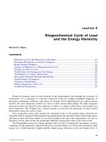
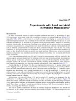
scale (Davis, 1993). The modified schematic extraction procedure for aquatic humic substances is
shown in Figure A6

A

.1. Details of the materials and methods used for the isolation and character-
ization of humic substances were described by Davis (1993).

DIALYSIS PROCEDURES FOR MEASURING LEAD BINDING
TO HUMIC SUBSTANCES

Equilibrium dialysis was used to determine the binding capacity of humic substances and
conditional stability constants (Saar and Weber, 1980). A continuous-flow system (Figure 6.6) was
selected to perform the equilibrium dialysis, as is popular in pharmaceutical processes (New, 1990).
A Spectrum Molecular/Por

®

Polysulfone, hollow fiber cartridge (HFC) was used to perform the
dialysis analysis. The HFC is a sturdy bundle composed of 90 hollow fibers with inside diameters
ranging from 0.5 to 0.7 mm and a molecular-weight cutoff at 2000 Da. The specifications of the
HFC feature a wide range of chemical compatibility and pH values, from 1 to 13.

Figure A6

A

.1

Sketch of procedure for extracting humic substances from water sample. (Modified from Ton, 1993.)
Filter sample through 0.45-µm
nylon filter; adjust pH to
2.0 with concentrated HCl
Non-humic
substances
XAD-8
resin
column
SpectraGel 50X8
cation exchange
resin column

Backwash
with 0.1 M
NaOH
Rinse with
2.0 M HCl
Discard
waste
Collect
sample;
lyophilize,
freeze-dry

L1401-frame-A6 Page 189 Tuesday, April 11, 2000 3:02 PM
© 2000 by CRC Press LLC

190 HEAVY METALS IN THE ENVIRONMENT: USING WETLANDS FOR THEIR REMOVAL

The bundle was securely placed into a cap assembly and housed in a 1000-ml polymethylpentene
(PMP) Fleaker

®

. A small 500-ml PMP Fleaker

®

was connected by Tygon

®

tubing to a Cole-Parmer
Masterflex

®

pump to circulate the process solution through fibers. The solution in the 1000-ml
Fleaker

®

also was circulated by pump. Two on-line sample outlets were installed to collect samples
during analysis, and two Fisher stirring plates were used to blend the samples. A diagram of the
apparatus used for dialysis analysis is shown in Figure 6.6. A test with lead on one side but without
organic matter reached an equilibrium with lead concentrations the same on both sides of the
membrane in 11 h or less (Figure A6

A

.2).
Two humic substances, Aldrich humic acid (AHA) and aquatic humic substances (SAPP 1),
were used to determine the Pb binding capacity of humic substances and the conditional stability
constants of Pb-organo complexes. Solutions of humic substances, AHA and SAPP 1 (approxi-
mately 20 mg humic substances per liter), were prepared in 0.1

M

KNO

3

(Saar and Weber, 1980).
Nitrogen gas was used to purge dissolved oxygen from the solutions before pH adjustment. The
pH of the solution was adjusted as needed using dilute HNO

3

and KOH solutions (in 0.1

M

KNO

3

).
One liter of organic solution was used for dialysis against 0.1 l of 0.1

M

KNO

3

for 72 h. Initially,
0.5 ml of 1000-mg/l Pb

2+

standard solution was added to the electrolyte to perform the dialysis
analysis, and 1.0 ml of 1000-mg/l Pb

2+

standard solution was added for overnight dialysis analysis.
Solutions were equilibrated for 6 h and 12 h in daytime overnight analyses, respectively, to assure
sufficient equilibration (Figure A6a.2). Before the next metal addition, equilibrated solutions were
subsampled (

circa

2 ml) through on-line sample outlets from both Fleakers. The Pb concentrations,
M

f

for free metal concentration and M

t

for total metal concentration in the equilibrated solutions,
were measured using flame atomic absorption spectrophotometry.

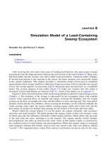
COMPLEXING CAPACITY DETERMINATION AND SCATCHARD
PLOT METHODOLOGY

When natural organic matter was dialyzed against a metal-ion solution, metal ions permeated
through the membrane of the fibers and formed complexed compounds in the Fleaker containing
organic matter (Alberts and Giesy, 1983; Saar and Weber, 1980; Stevenson, 1982; Truitt and Weber,
1981a, 1981b; Tuschall, 1981; Weber, 1983). At equilibrium, the free-metal concentration M

f

was
measured in the Fleaker containing electrolyte. Total metal concentration M

t

, free plus complexed,
was measured in the Fleaker containing organic matter. The complexed metal M

c

then was calculated
by a simple mass-balance equation:

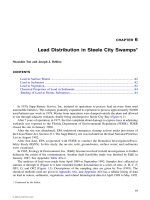
Figure A6

A

.2

Example of the lead binding by humic substances in the dialysis apparatus (Figure A6

A

.1).
Equilibrium level is used to evaluate coefficients of dissociation (Ton, 1993).
Hours
0 1 2 3 4 5 6 7 8 9
0

0.2
0.4
0.6
0.8
1.0
1.2
1.4
Equilibrium conc. = 1.1 mg/l
pH 3.0
Permeate concentration, mg/l

L1401-frame-A6 Page 190 Tuesday, April 11, 2000 3:02 PM
© 2000 by CRC Press LLC

METHODS USED FOR CHEMICAL ANALYSIS OF WATERS AND SEDIMENTS 191

M

c

= M

t

– M

f

The Pb complexing capacity was obtained from a plot of freely dissolved Pb concentration vs.
total Pb concentration. The curve was extrapolated to the abscissa in order to obtain the Pb

complexing capacity (Davis, 1993; Truitt and Weber, 1981a).
The conditional stability constant (

β

) can be estimated using the Scatchard method (Stevenson,
1982; Tuschall, 1981). It was assumed that
where A

T

is the total ligand concentration, in terms of humic substances, and n is the number of
binding sites per ligand molecule.
The equation above can be rearranged to
By substituting V for M

c

/A

T

, the final form of the equation becomes
Thus, a plot of M

c

/M

f

vs. V should produce a curve with slope –

β

. This data analysis has been
attributed to Scatchard, and a plot of V/M

f

vs. V is termed a Scatchard plot (Stevenson, 1982;
Tuschall, 1981). A theoretical Scatchard plot for titration of organic matter with metal is given in
Figure A6

A

.3. The illustrated approach suggests two categories of

β

, with one “strong” site and

Figure A6

A

.3

Theoretical Scatchard plot used to evaluate stability constants (Ton, 1993).
β

M
c
M
f
()nA
T
M
c
–()
=
M
c
M
f
()A
T
()
β n
M
c
A
T
–=
V
M
f
β nV–()=
Slope = - B
a
("strong"site)

V/M
f
Slope = -B
b
("Weak" site)
V = (Metal complexed, M
c
)/(Total ligand, AT)

L1401-frame-A6 Page 191 Tuesday, April 11, 2000 3:02 PM
© 2000 by CRC Press LLC

192 HEAVY METALS IN THE ENVIRONMENT: USING WETLANDS FOR THEIR REMOVAL

one “weak” site. Changes of b in aqueous humic-substance samples (SAPP 1) with different pH
values were examined.
A potential problem with the equilibrium dialysis technique is the leakage of humic substances
across the membrane. This would lead to an underestimation of the Pb binding capacity and
conditional stability constants (Truitt and Weber, 1981a). Lowered accuracy and reproducibility of
analytical measurements further increased the uncertainty for metal binding capacities and deter-
minations of stability constants (Haworth et al., 1987).

L1401-frame-A6 Page 192 Tuesday, April 11, 2000 3:02 PM
© 2000 by CRC Press LLC

193

A

PPENDIX

A6

B

Chemical Data on the Cypress-Gum Swamps
of Steele City Bay, Jackson County, Florida

Shanshin Ton and Joseph J. Delfino

This appendix contains data tables on the area studied for lead uptake. The analyses were
first made at six stations (A, B, C, D, F, G) shown in Figure 6.1, where A is closest to the
battery washing site. Later, sampling sites were expanded further downstream in a series of
sites (A, B, C, F, OF1, OF2). Descriptions are given by Ton (1993). Sampling sites OF1 and
OF2 were designated as checkout points for the Steele Bay Swamps and the boundary of the
study area, respectively.

L1401-frame-A6b Page 193 Tuesday, April 11, 2000 3:05 PM
© 2000 by CRC Press LLC

194 HEAVY METALS IN THE ENVIRONMENT: USING WETLANDS FOR THEIR REMOVAL

Table A6

B

.2 Concentrations of Pb in a Wetland that Received Dischar
ges from the Sapp Battery Superfund Site and in a Nearb
y Freshwater

Wetland
Background
Data

a

Livingston (1983–1985)

E & E (1986) Report

E & E (1989) Report
Station 1

b

Station 2 E. Swamp
Steele City
Bay E. Swamp
Steele City
Bay

Surface water (mg/l) 0.01 0.41–4.55 0.25–0.80 0.03 0.06 0.06 0.02
Sediments (

µ

g/g) 9.0 184–1939 20.5–999.5 78.6 24–820 NA 33–940
Vegetation (

µ

g/g) 8.00

c

NA NA NA NA NA NA

Note:

NA = not available.

a

Data cited from E & E (1985) study.

b

The locations in this table do not refer to sampling site.

c

Data cited from Casagrande and Erchull (1977), Okefenokee Swamp, Georgia.

L1401-frame-A6b Page 194 Tuesday, April 11, 2000 3:05 PM
© 2000 by CRC Press LLC

CHEMICAL DATA ON THE CYPRESS-GUM SWAMPS OF STEELE CITY BAY 195

Table A6

B

.3 Water Quality of Sampling Sites that Received Discharge from the Sapp Battery

Superfund Site, Jackson County, Florida
A

a

BCD F G
Background
Data

b

Distance (m)

c

0 40 244 387 259 >600 —
pH 3.4 3.6 3.8 4.4 4.5 3.9 4.3–5.0
Temperature (°C) 32 31 32 28 29.5 ——
Water depth (cm) 51 52 63–89 >90 38–51 31–51 —
Conductivity
(

µ

mho/cm–25°C)
22 106 76 31 47.5 76.5 60–70

Nitrite + nitrate (mg-N/l) 0.08 0.01 0.02 0.04 0.04 0.02 0.005–0.11
Ammonia (mg-N/l) 3.76 0.18 0.08 0.16 0.35 0.16 0.01–0.56
Total Kjeldahl N (mg/l) 5.08 1.43 2.06 3.60 2.31 1.08 1.04–1.71
Total P (mg/l) 0.03 0.07 0.09 0.20 0.08 0.02 0.05–0.16
Total Pb (mg/l) 0.28 0.03 <0.01 <0.01 0.01 0.01 —

Note:

— indicates no data; mg/l = ppm.

a

See Figure 5.2 for the locations of the sampling sites.

b

Background data are cited from Ewel and Odum, 1984.

c

Distance measured from County Road 280. 0 m indicates inside the source area.

Table A6

B

.4 pH and Electrical Conductivity, 1989–1992
Site
Apr
1989

Feb
1990
Aug
1990
Sept
1990
June
1991
Jan
1992
May
1992 Avg SD Max Min

pH in Surface Water

A 3.4 ———3.6 4.2 3.5 3.7 0.37 4.2 3.4
A0 ——————3.9 3.9 — 3.9 3.9
B 3.6 3.9 4.1 3.8 4.2 4.9 4.1 4.1 0.42 4.9 3.6
C 3.8 — 3.7 4.0 4.2 4.8 4.0 4.1 0.37 4.8 3.7
D 4.5 — 4.2 — 4.3 5.0 4.6 4.5 0.32 5.0 4.2
E — 3.9 ——4.8 5.2 4.4 4.6 0.56 5.2 3.9
F 4.5 — 3.8 — 4.3 5.5 4.6 4.5 0.62 5.5 3.8
G 3.9 — 4.6 — 4.4 4.9 4.8 4.5 0.39 4.9 3.9
H ——5.0 — 5.0 5.8 4.6 5.1 0.50 5.8 4.6
OF1 ———4.0 4.2 5.9 5.0 4.8 0.87 5.9 4.0
OF2 ———3.8 4.5 4.6 4.5 4.3 0.36 4.6 3.8
PC ————4.9 7.0 5.0 5.6 1.20 7.0 4.9

Electrical Conductivity in Surface Water (S/cm)

A 322.0 ———42.3 180.0 139.7 171.0 116.1 322.0 42.3
A0 ——————61.0 61.0 — 61.0 61.0
B 106.0 — 38.3 4.9 34.0 49.6 40.5 55.5 27.05 106.0 34.0
C 76.4 — 46.9 44.6 27.0 37.0 36 44.6 17.06 76.4 27.0
D 30.8 — 28.6 — 23.2 28.0 30.7 28.3 3.09 30.8 23.2
E ————29.2 65.2 43.4 45.9 18.13 65.2 29.2
F 47.4 — 61.3 — 30.5 48.0 32 43.8 12.76 61.3 30.5
G 76.5 — 100.1 — 27.0 46.6 28 55.6 31.92 100.1 27.0
H ——72.7 — 31.6 45.0 42 47.8 17.55 72.7 31.6
OF1 ———39.7 25.0 32.0 34 32.7 6.05 39.7 25.0
OF2 ———56.8 25.5 67.4 26.8 44.1 21.21 67.4 25.5
PC ————29.5 46.7 40 38.7 8.67 46.7 29.5

L1401-frame-A6b Page 195 Tuesday, April 11, 2000 3:05 PM
© 2000 by CRC Press LLC

196 HEAVY METALS IN THE ENVIRONMENT: USING WETLANDS FOR THEIR REMOVAL

Table A6

B

.5 Lead in Surface Water, Sediment, and Animals (Ton, 1993)
Site
Apr
1989
Feb
1990
Aug
1990

Jan
1992
May
1992 Avg SD Max Min

Lead in Surface Water (mg/l)

A 0.28 — 0.01 0.14 0.09 0.13 0.11 0.3 0.0
A0 ———<0.01 0.01 0.01 0.00 0.0 0.0
B 0.03 0.01 0.02 0.01 0.01 0.02 0.01 0.0 0.0
C <0.01 0.01 <0.01 <0.01 0.01 0.01 0.00 0.0 0.0
D <0.01 <0.01 0.01 <0.01 <0.01 0.01 0.00 0.0 0.0
E ——0.01 0.20 0.06 0.09 0.10 0.2 0.0
F 0.01 0.01 <0.01 0.01 <0.01 0.01 0.00 0.0 0.0
G <0.01 0.01 <0.01 <0.01 <0.01 0.01 0.00 0.0 0.0
H — 0.03 0.01 <0.01 <0.01 0.02 0.01 0.0 0.0
OF1 ——<0.01 <0.01 <0.01 <0.01 0.00 0.0 0.0
OF2 ——<0.01 <0.01 <0.01 <0.01 0.00 0.0 0.0
PC ——<0.01 <0.01 <0.01 <0.01 0.00 0.0 0.0

Lead in Sediments (

µ

g/g)

A 385.7 — 393.9 27.7 23.4 207.7 210.3 393.9 23.4
A0 ————36.2 36.2 0.0 36.2 36.2
B 210.9 — 763.7 113.0 74.5 290.5 320.6 763.7 74.5
C 234.2 — 278.9 23.5 48.8 146.3 129.0 278.9 23.5

D 59.4 — 303.6 10.6 49.2 105.7 133.6 303.6 10.6
E — 477.8 — 342.1 512.0 444.0 89.8 512.0 342.1
F 88.5 — 472.2 99.9 125.7 196.6 184.4 472.2 88.5
G 94.3 — 99.6 87.4 62.0 85.8 16.7 99.6 62.0
H ——215.7 36.3 112.9 121.6 90.0 215.7 36.3
OF1 — 133.3 — 23.5 10.6 55.8 67.4 133.3 10.6
OF2 ———10.6 10.6 10.6 0.1 10.6 10.6
PC ———23.3 23.4 23.4 0.0 23.4 23.3

Lead in Animals, October 1989 (

µ

g/g)

Beaver (

Castor fiber

) Site L 13.3 (liver)
Sunfish(

Centrarchus

) Site F 66.7
Sunfish (

Centrarchus

) Site F 50.0

Pickeral (

Esox lucius

) Site G 16.7

L1401-frame-A6b Page 196 Tuesday, April 11, 2000 3:05 PM
© 2000 by CRC Press LLC