Sediment and Contaminant Transport in Surface Waters - Chapter 1 ppt
Bạn đang xem bản rút gọn của tài liệu. Xem và tải ngay bản đầy đủ của tài liệu tại đây (779.22 KB, 31 trang )
Sediment
and
Contaminant
Transport
in
Surface
Waters
© 2009 by Taylor & Francis Group, LLC
CRC Press is an imprint of the
Taylor & Francis Group, an informa business
Boca Raton London New York
Sediment
and
Contaminant
Transport
in
Surface
Waters
WILBERT LICK
© 2009 by Taylor & Francis Group, LLC
CRC Press
Taylor & Francis Group
6000 Broken Sound Parkway NW, Suite 300
Boca Raton, FL 33487-2742
© 2009 by Taylor & Francis Group, LLC
CRC Press is an imprint of Taylor & Francis Group, an Informa business
No claim to original U.S. Government works
Printed in the United States of America on acid-free paper
10 9 8 7 6 5 4 3 2 1
International Standard Book Number-13: 978-1-4200-5987-8 (Hardcover)
This book contains information obtained from authentic and highly regarded sources. Reasonable efforts
have been made to publish reliable data and information, but the author and publisher cannot assume
responsibility for the validity of all materials or the consequences of their use. The authors and publishers
have attempted to trace the copyright holders of all material reproduced in this publication and apologize
to copyright holders if permission to publish in this form has not been obtained. If any copyright material
has not been acknowledged please write and let us know so we may rectify in any future reprint.
Except as permitted under U.S. Copyright Law, no part of this book may be reprinted, reproduced, trans-
mitted, or utilized in any form by any electronic, mechanical, or other means, now known or hereafter
invented, including photocopying, microfilming, and recording, or in any information storage or retrieval
system, without written permission from the publishers.
For permission to photocopy or use material electronically from this work, please access www.copyright.
com ( or contact the Copyright Clearance Center, Inc. (CCC), 222 Rosewood
Drive, Danvers, MA 01923, 978-750-8400. CCC is a not-for-profit organization that provides licenses and
registration for a variety of users. For organizations that have been granted a photocopy license by the
CCC, a separate system of payment has been arranged.
Trademark Notice: Product or corporate names may be trademarks or registered trademarks, and are
used only for identification and explanation without intent to infringe.
Library of Congress Cataloging-in-Publication Data
Lick, Wilbert J.
Sediment and contaminant transport in surface waters / author, Wilbert Lick.
p. cm.
“A CRC title.”
Includes bibliographical references.
ISBN 978-1-4200-5987-8 (alk. paper)
1. Water Pollution. 2. Sediment transport. 3. Contaminated sediments. 4.
Streamflow. 5. Limnology. 6. Environmental geochemistry. I. Title.
TD425.L52 2009
628.1’68 dc22 2008023728
Visit the Taylor & Francis Web site at
and the CRC Press Web site at
© 2009 by Taylor & Francis Group, LLC
v
Contents
Preface xiii
About the Author xv
Chapter 1 Introduction 1
1.1 Examples of Contaminated Sediment Sites 2
1.1.1 Hudson River 2
1.1.2 Lower Fox River 4
1.1.3 Passaic River/Newark Bay 6
1.1.4 Palos Verdes Shelf 7
1.2 Modeling, Parameterization, and Non-Unique Solutions 9
1.2.1 Modeling 9
1.2.2 Parameterization and Non-Unique Solutions 10
1.3 The Importance of Big Events 12
1.4 Overview of Book 17
Chapter 2 General Properties of Sediments 21
2.1 Particle Sizes 21
2.1.1 Classication of Sizes 21
2.1.2 Measurements of Particle Size 23
2.1.3 Size Distributions 23
2.1.4 Variations in Size of Natural Sediments throughout a System 26
2.2 Settling Speeds 30
2.3 Mineralogy 33
2.4 Flocculation of Suspended Sediments 35
2.5 Bulk Densities of Bottom Sediments 37
2.5.1 Measurements of Bulk Density 39
2.5.2 Variations in Bulk Density 41
Chapter 3 Sediment Erosion 45
3.1 Devices for Measuring Sediment Resuspension/Erosion 46
3.1.1 Annular Flumes 46
3.1.2 The Shaker 50
3.1.3 Sedume 51
3.1.4 A Comparison of Devices 54
3.2 Results of Field Measurements 56
3.2.1 Detroit River 57
3.2.2 Kalamazoo River 60
© 2009 by Taylor & Francis Group, LLC
vi Sediment and Contaminant Transport in Surface Waters
3.3 Effects of Bulk Properties on Erosion Rates 67
3.3.1 Bulk Density 68
3.3.2 Particle Size 70
3.3.3 Mineralogy 72
3.3.4 Organic Content 75
3.3.5 Salinity 76
3.3.6 Gas 77
3.3.7 Comparison of Erosion Rates 79
3.3.8 Benthic Organisms and Bacteria 80
3.4 Initiation of Motion and a Critical Shear Stress for Erosion 81
3.4.1 Theoretical Analysis for Noncohesive Particles 83
3.4.2 Effects of Cohesive Forces 85
3.4.3 Effects of Bulk Density 87
3.4.4 Effects of Clay Minerals 88
3.5 Approximate Equations for Erosion Rates 90
3.5.1 Cohesive Sediments 90
3.5.2 Noncohesive Sediments 91
3.5.3 A Uniformly Valid Equation 92
3.5.4 Effects of Clay Minerals 92
3.6 Effects of Surface Slope 93
3.6.1 Noncohesive Sediments 93
3.6.2 Critical Stresses for Cohesive Sediments 96
3.6.3 Experimental Results for Cohesive Sediments 97
Chapter 4 Flocculation, Settling, Deposition, and Consolidation 103
4.1 Basic Theory of Aggregation 104
4.1.1 Collision Frequency 104
4.1.2 Particle Interactions 106
4.2 Results of Flocculation Experiments 108
4.2.1 Flocculation due to Fluid Shear 109
4.2.2 Flocculation due to Differential Settling 116
4.3 Settling Speeds of Flocs 120
4.3.1 Flocs Produced in a Couette Flocculator 120
4.3.2 Flocs Produced in a Disk Flocculator 122
4.3.3 An Approximate and Uniformly Valid Equation for the
Settling Speed of a Floc 125
4.4 Models of Flocculation 126
4.4.1 General Formulation and Model 126
4.4.2 A Simple Model 130
4.4.3 A Very Simple Model 138
4.4.3.1 An Alternate Derivation 139
4.4.4 Fractal Theory 140
© 2009 by Taylor & Francis Group, LLC
Contents vii
4.5 Deposition 142
4.5.1 Processes and Parameters That Affect Deposition 145
4.5.1.1 Fluid Turbulence 145
4.5.1.2 Particle Dynamics 148
4.5.1.3 Particle Size Distribution 148
4.5.1.4 Flocculation 148
4.5.1.5 Bed Armoring/Consolidation 149
4.5.1.6 Partial Coverage of Previously Deposited Sediments
by Recently Deposited Sediments 149
4.5.2 Experimental Results and Analyses 149
4.5.3 Implications for Modeling Deposition 154
4.6 Consolidation 155
4.6.1 Experimental Results 156
4.6.2 Basic Theory of Consolidation 165
4.6.3 Consolidation Theory Including Gas 169
Appendix A 171
Appendix B 172
Chapter 5 Hydrodynamic Modeling 175
5.1 General Considerations in the Modeling of Currents 176
5.1.1 Basic Equations and Boundary Conditions 176
5.1.2 Eddy Coefcients 179
5.1.3 Bottom Shear Stress 182
5.1.3.1 Effects of Currents 182
5.1.3.2 Effects of Waves and Currents 185
5.1.4 Wind Stress 187
5.1.5 Sigma Coordinates 188
5.1.6 Numerical Stability 189
5.2 Two-Dimensional, Vertically Integrated, Time-Dependent Models 190
5.2.1 Basic Equations and Approximations 190
5.2.2 The Lower Fox River 191
5.2.3 Wind-Driven Currents in Lake Erie 194
5.3 Two-Dimensional, Horizontally Integrated, Time-Dependent Models . 195
5.3.1 Basic Equations and Approximations 196
5.3.2 Time-Dependent Thermal Stratication in Lake Erie 198
5.4 Three-Dimensional, Time-Dependent Models 201
5.4.1 Lower Duwamish Waterway 202
5.4.1.1 Numerical Error due to Use of Sigma Coordinates 204
5.4.1.2 Model of Currents and Salinities 205
5.4.2 Flow around Partially Submerged Cylindrical Bridge Piers 206
5.5 Wave Action 210
5.5.1 Wave Generation 210
© 2009 by Taylor & Francis Group, LLC
viii Sediment and Contaminant Transport in Surface Waters
5.5.2 Lake Erie 211
5.5.2.1 A Southwest Wind 212
5.5.2.2 A North Wind 213
5.5.2.3 Relation of Wave Action to Sediment Texture 213
Chapter 6 Modeling Sediment Transport 215
6.1 Overview of Models 215
6.1.1 Dimensions 215
6.1.2 Quantities That Signicantly Affect Sediment Transport 216
6.1.2.1 Erosion Rates 216
6.1.2.2 Particle/Floc Size Distributions 217
6.1.2.3 Settling Speeds 218
6.1.2.4 Deposition Rates 219
6.1.2.5 Flocculation of Particles 219
6.1.2.6 Consolidation 219
6.1.2.7 Erosion into Suspended Load and/or Bedload 220
6.1.2.8 Bed Armoring 220
6.2 Transport as Suspended Load and Bedload 220
6.2.1 Suspended Load 220
6.2.2 Bedload 221
6.2.3 Erosion into Suspended Load and/or Bedload 223
6.2.4 Bed Armoring 226
6.3 Simple Applications 226
6.3.1 Transport and Coarsening in a Straight Channel 227
6.3.2 Transport in an Expansion Region 229
6.3.3 Transport in a Curved Channel 235
6.3.4 The Vertical Transport and Distribution of Flocs 237
6.4 Rivers 239
6.4.1 Sediment Transport in the Lower Fox River 239
6.4.1.1 Model Parameters 240
6.4.1.2 A Time-Varying Flow 242
6.4.2 Upstream Boundary Condition for Sediment Concentration 246
6.4.3 Use of Sedume Data in Modeling Erosion Rates 249
6.4.4 Effects of Grid Size 251
6.4.5 Sediment Transport in the Saginaw River 252
6.4.5.1 Sediment Transport during Spring Runoff 255
6.4.5.2 Long-Term Sediment Transport Predictions 257
6.5 Lakes and Bays 261
6.5.1 Modeling Big Events in Lake Erie 261
6.5.1.1 Transport due to Uniform Winds 261
6.5.1.2 The 1940 Armistice Day Storm 263
6.5.1.3 Geochronology 264
6.5.2 Comparison of Sediment Transport Models for Green Bay 266
© 2009 by Taylor & Francis Group, LLC
Contents ix
6.6 Formation of a Turbidity Maximum in an Estuary 271
6.6.1 Numerical Model and Transport Parameters 272
6.6.2 Numerical Calculations 273
6.6.2.1 A Constant-Depth, Steady-State Flow 273
6.6.2.2 A Variable-Depth, Steady-State Flow 274
6.6.2.3 A Variable-Depth, Time-Dependent Tidal Flow 277
Chapter 7 The Sorption and Partitioning of Hydrophobic Organic
Chemicals 279
7.1 Experimental Results and Analyses 280
7.1.1 Basic Experiments 280
7.1.2 Parameters That Affect Steady-State Sorption and Partitioning 285
7.1.2.1 Colloids from the Sediments 285
7.1.2.2 Colloids from the Water 289
7.1.2.3 Organic Content of Sediments 291
7.1.2.4 Sorption to Benthic Organisms and Bacteria 292
7.1.3 Nonlinear Isotherms 292
7.2 Modeling the Dynamics of Sorption 297
7.2.1 A Diffusion Model 298
7.2.2 A Simple and Computationally Efcient Model 300
7.2.3 Calculations with the General Model and Comparisons with
Experimental Results 303
7.2.3.1 Desorption 305
7.2.3.2 Adsorption 308
7.2.3.3 Short-Term Adsorption Followed by Desorption 310
7.2.3.4 Effects of Chemical Properties on Adsorption 311
Chapter 8 Modeling the Transport and Fate of Hydrophobic Chemicals 313
8.1 Effects of Erosion/Deposition and Transport 316
8.1.1 The Saginaw River 316
8.1.2 Green Bay, Effects of Finite Sorption Rates 319
8.2 The Diffusion Approximation for the Sediment-Water Flux 322
8.2.1 Simple, or Fickian, Diffusion 322
8.2.2 Sorption Equilibrium 325
8.2.3 A Mass Transfer Approximation 326
8.3 The Sediment-Water Flux due to Molecular Diffusion 327
8.3.1 Hexachlorobenzene (HCB) 328
8.3.1.1 Experiments 328
8.3.1.2 Theoretical Models 329
8.3.1.3 Diffusion of Tritiated Water 330
8.3.1.4 HCB Diffusion and Sorption 331
© 2009 by Taylor & Francis Group, LLC
x Sediment and Contaminant Transport in Surface Waters
8.3.2 Additional HOCs 334
8.3.2.1 Experimental Results 334
8.3.2.2 Theoretical Model 336
8.3.2.3 Numerical Calculations 337
8.3.3 Long-Term Sediment-Water Fluxes 338
8.3.4 Related Problems 338
8.3.4.1 Flux from Contaminated Bottom Sediments to
Clean Overlying Water 338
8.3.4.2 Flux Due to a Contaminant Spill 341
8.4 The Sediment-Water Flux Due to Bioturbation 342
8.4.1 Physical Mixing of Sediments by Organisms 343
8.4.2 The Flux of an HOC Due to Organisms 344
8.4.2.1 Experimental Procedures 345
8.4.2.2 Theoretical Model 346
8.4.2.3 Experimental and Modeling Results 348
8.4.3 Modeling Bioturbation as a Diffusion with Finite-Rate
Sorption Process 353
8.5 The Sediment-Water Flux Due to “Diffusion” 355
8.5.1 The Flux and the Formation of Sediment Layers Due to
Erosion/Deposition 355
8.5.2 Comparison of “Diffusive” Fluxes and Decay Times 356
8.5.3 Observations of Well-Mixed Layers 357
8.5.4 The Determination of an Effective h 359
8.6 Environmental Dredging: A Study of Contaminant Release and
Transport 360
8.6.1 Transport of Dredged Particles 361
8.6.2 Transport and Desorption of Chemical Initially Sorbed to
Dredged Particles 362
8.6.3 Diffusive Release of Contaminant from the Residual Layers 363
8.6.4 Volatilization 365
8.7 Water Quality Modeling, Parameterization, and Non-Unique
Solutions 366
8.7.1 Process Models 367
8.7.1.1 Sediment Erosion 367
8.7.1.2 Sediment Deposition 367
8.7.1.3 Bed Armoring 368
8.7.1.4 The Sediment-Water Flux of HOCs Due to “Diffusion” 368
8.7.1.5 Equilibrium Partitioning 368
8.7.1.6 Numerical Grid 369
8.7.2 Parameterization and Non-Unique Solutions 369
8.7.3 Implications for Water Quality Modeling 370
References 373
© 2009 by Taylor & Francis Group, LLC
xi
Dedication
To
Jim and Sarah
© 2009 by Taylor & Francis Group, LLC
xiii
Preface
This book began as brief sets of notes prepared for a graduate class of students
at the University of California at Santa Barbara (UCSB). The course emphasized
the transport of sediments and contaminants in surface waters. The students were
mainly from engineering, but there also were students from the departments of
environmental sciences and biology. The course was later given twice as a short
course (with the same emphasis) in Santa Barbara to professionals in the eld,
primarily to personnel from the U.S. Environmental Protection Agency and the
U.S. Army Corps of Engineers but also to personnel from other federal and state
agencies, consulting companies, and educational institutions.
Sediment and contaminant transport is an enormously rich and complex eld
and involves physical, chemical, and biological processes as well as the math-
ematical modeling of these processes. Many books and articles have been written
on the general topic, and much work is currently being done in this area. Rather
than review this extremely large set of investigations, the emphasis here is on top-
ics that have been recently investigated and not covered thoroughly elsewhere —
for example, the erosion, deposition, occulation, and transport of ne-grained,
cohesive sediments; the effects of nite rates of sorption on the transport and fate
of hydrophobic contaminants; and the effects of big events such as oods and
storms. Despite this emphasis, the overall goal is to present a general descrip-
tion and understanding of the transport of sediments and contaminants in surface
waters as well as procedures to quantitatively predict this transport.
Much of the work described in this book is based on the research done by
graduate students and post-doctoral fellows in the author’s research group at
UCSB and previously at Case Western Reserve University. For their work, inspi-
ration, and input, I am enormously grateful. Because they are quite numerous,
it is difcult to list them with their specic contributions here; hopefully, I have
thoroughly referenced their contributions in the text itself. I am also grateful to
June Finney, who did much of the typing and assisted in many other ways. Sev-
eral researchers (Lawrence Burkhard, USEPA; Earl Hayter, U.S. Army Corps of
Engineers; Doug Endicott, Great Lakes Environmental Center; and Craig Jones,
Sea Engineering) have each reviewed two or more chapters of the text. Their com-
ments and suggestions were of great help.
© 2009 by Taylor & Francis Group, LLC
xv
About the Author
Wilbert Lick is currently a research professor in the Department of Mechanical
and Environmental Engineering at the University of California at Santa Barbara
(UCSB). His main expertise is in the environmental sciences, uid mechanics,
mathematical modeling, and numerical methods. His present interests are in
understanding and predicting the transport and fate of sediments and contami-
nants in surface and ground waters and the effects of these processes on water
quality. This work involves laboratory experiments and numerical modeling with
some eldwork for testing devices and data verication. He has researched these
problems in the Great Lakes, the Santa Barbara Channel, New York Harbor, Long
Beach Harbor, the Venice Lagoon in Italy, and Korea.
Lick is the author of more than 100 peer-reviewed articles and is a consultant
to federal and state agencies as well as private companies. Previous to UCSB, he
taught at Harvard University and Case Western Reserve University, with visiting
appointments at the California Institute of Technology and Imperial College, Uni-
versity of London. His Ph.D. is from Rensselaer Polytechnic Institute.
© 2009 by Taylor & Francis Group, LLC
1
1
Introduction
The general purpose of this text is to assist in the quantitative understanding of
and ability to predict the transport of sediments and hydrophobic contaminants
in surface waters. For this reason, fundamental processes are emphasized and
described. However, any attempt to understand and predict sediment and con-
taminant transport inevitably leads to mathematical models, occasionally simple
conceptual or analytical models, but often more complex numerical models. Two
of the main limitations in the usefulness of these models are (1) an inadequate
knowledge of the processes included in the models and (2) an inadequate ability
to approximate and/or parameterize these processes. For these reasons, approxi-
mately half of the text is a presentation and discussion of basic processes that are
signicant and that need to be quantitatively understood to develop quantitative
and accurate models of sediment and contaminant transport; the other half of the
text is the development, description, and application of these models. Throughout,
the emphasis is on realistic descriptions of sediments (e.g., cohesive, ne-grained
sediments as well as non-cohesive, coarse-grained sediments); contaminants
(nite sorption rates); and environmental conditions (including big events).
The most obvious application of the work described here is to the problem of
contaminated bottom sediments. These sediments and their negative impacts on
water quality are a major problem in surface waters throughout the United States
as well as in many other parts of the world. Even after elimination of the primary
contaminant sources, these bottom sediments will be a major source of contami-
nants for many years to come. To determine environmentally effective and cost-
effective remedial actions, the transport and fate of these sediments and associated
contaminants must be understood and quantied. More generally, the transport and
fate of sediments and contaminants are basic processes that must be understood
for assessing water quality and health issues (toxic transport and fate, bioaccumu-
lation); water body management (navigation, dredging, recreation); and potential
remediation methods (environmental dredging, capping, natural recovery).
Examples of surface waters that are heavily impacted by contaminated bot-
tom sediments are the Hudson River, the Lower Fox River, the Passaic River/
Newark Bay Estuary, and the Palos Verdes Shelf. These sites are all similar
in that they are locations of historical industrial discharges; large amounts of
contaminated sediments are still present; and, because of the toxicity and per-
sistence of the chemicals and the large amounts of contaminated sediments,
there is considerable uncertainty on how best to remediate each site. For each
site, extensive descriptions of the site; the contaminated sediment problem;
and the scientic, engineering, and political issues that arise in the solution
© 2009 by Taylor & Francis Group, LLC
2 Sediment and Contaminant Transport in Surface Waters
of the problem are given on the Web by the U.S. Environmental Protection
Agency (EPA) as well as other organizations. Brief descriptions of these sites,
the problems due to contaminated sediments at these sites, and progress toward
remediation are given in the following section. Most of this information is from
EPA listings on the Web.
In the description of the transport of sediment and contaminant transport
and in water quality models in general, numerous parameters appear; many of
these parameters may not be well understood or quantied. When they cannot
be adequately determined directly from laboratory or eld data, they often are
determined by parameterization (also called model calibration) — that is, by
varying the value of each parameter until the solution, however dened, ts some
observed quantity. Although quite useful, there are limitations to this procedure,
especially when multiple parameters are involved. For this reason, a preliminary
discussion of modeling, the determination of parameters needed in the modeling,
and the associated problem of non-unique solutions are given in Section 1.2.
Big events, such as large storms and oods, have been shown to have a major
effect on the transport and fate of sediments and contaminants and, hence, on
water quality. This is a recurring theme throughout the text. An introduction to
this topic is given in Section 1.3, and an overview of the entire book is given in
Section 1.4.
1.1 EXAMPLES OF CONTAMINATED SEDIMENT SITES
1.1.1 H
UDSON RIVER
The Hudson River is located in New York State and ows from its source in
the Adirondack Mountains south approximately 510 km to Manhattan Island and
the Atlantic Ocean. Much of the river is contaminated by polychlorinated biphe-
nyls (PCBs), and the contaminated part of the river has been designated as a
Superfund site. This site extends approximately 320 km from Hudson Falls to
Manhattan Island and is the largest and most expensive Superfund site involv-
ing contaminated sediments. For descriptive purposes, the site has been further
divided into the Upper Hudson (from Hudson Falls to the Federal Dam at Troy,
approximately 64 km, Figure 1.1) and the Lower Hudson River (from the Federal
Dam to Manhattan Island). The Upper Hudson contains the highest concentra-
tions of PCBs.
The PCB contamination is primarily due to the release of PCBs from two
General Electric Company (GE) capacitor plants in the Upper Hudson at Fort
Edward and Hudson Falls. At these two plants, GE used PCBs in the manufacture
of electrical capacitors from approximately 1947 to 1977. During this time, as
much as 600,000 kg of PCBs were discharged into the Hudson. The use of PCBs
was discontinued in 1977; since then, additional PCBs have leaked into the Hud-
son River from the Hudson Falls plant through cracks in the bedrock.
The primary health risk associated with PCBs in the Hudson River is the
accumulation of PCBs in the human body through eating contaminated sh.
© 2009 by Taylor & Francis Group, LLC
Introduction 3
PCBs are considered probable human carcinogens and are linked to other adverse
health effects such as low birth weight; thyroid disease; and learning, memory, and
immune system disorders. PCBs have similar effects on sh and other wildlife.
Because of their hydrophobicity, PCBs sorb to sediments, are transported
with them, and settle with them in areas of low ow (e.g., behind dams). Many of
the sorbed PCBs settled initially behind the Fort Edward Dam just downstream
of Hudson Falls (Figure 1.1). Because the dam was deteriorating and was in poor
condition, the Niagara Mohawk Power Corporation removed the dam in 1973.
During subsequent spring oods and other high ow periods, the PCB-contami-
nated sediments behind the dam were eroded, transported downstream, and again
Glens
Falls
Hudson
Falls
Fort Edward
RM 190
TIP
RM 200
RM 180
RM 170
0 5 mi
N
0 10 k
RM 160
Waterford
Troy
Cohoes
Mechanicville
RM 210
FIGURE 1.1 Upper Hudson River.
© 2009 by Taylor & Francis Group, LLC
4 Sediment and Contaminant Transport in Surface Waters
deposited in low-owing and quiescent areas of the river (including areas behind
downstream dams).
Areas with potentially high PCB concentrations were surveyed by the New
York State Department of Environmental Conservation from 1976 to 1978 and
again in 1984. Areas that generally had PCB concentrations greater than 50 mg/kg
were dened as “hot spots.” Approximately half of these hot spots were located in
the Thompson Island Pool (TIP) behind Thompson Island Dam (Figure 1.1).
Since 1976, because of high levels of PCBs in sh, New York State has closed
recreational and commercial sheries and has issued advisories restricting the
consumption of sh caught in the Hudson River. In addition, extensive investiga-
tions of PCB concentrations, their transport and fate, their uptake by organisms,
and subsequent transfer through the food chain have been made by GE (e.g., QEA,
1999) and EPA by means of eld measurements, laboratory analyses, and numeri-
cal modeling. In 2005, the Department of Justice and EPA reached an agreement
with GE that required GE to begin remediation of contaminated sediments in the
Thompson Island Pool. Proposed remediation is by a combination of dredging,
capping, and natural recovery. Dredging is scheduled to begin in spring 2008.
Approximately 2.5 × 10
6
m
3
of sediment and 7 × 10
4
kg of PCBs will be removed.
The expected cost of the dredging is more than $700 million.
1.1.2 LOWER FOX RIVER
The Lower Fox River is in Wisconsin, is 63 km long, and runs from Lake Win-
nebago in the south to Green Bay in the north. It is similar to the Hudson River
in that it is a Superfund site due to PCB contamination of the bottom sediments.
However, compared to the Hudson, it is smaller in length, its volume ow rate is
lower, and its sediments contain a smaller amount of PCBs; however, PCB con-
centrations are similar.
Over the distance from Lake Winnebago to Green Bay, the river drops by
52 m. To develop water power and improve navigation, the U.S. Army Corps of
Engineers constructed a series of 17 locks and dams on the Fox; this construction
was completed in 1884 and allowed navigation from the Great Lakes through the
Fox to the Mississippi River. In the downstream direction from Lake Winnebago
to Green Bay, the last dam in the series is at DePere (Figure 1.2). Dredging of the
river below this dam for navigation purposes has caused the river in this area to
be wide and deep. As a consequence, the ow velocities there are relatively low
and sediment deposition is high. It is estimated that 75% of the present sediment
deposition in the Lower Fox occurs between DePere Dam and Green Bay.
The combination of cheap water transportation and power attracted a large
number of industries, including manufacturers of wood products and paper mills.
This area is considered to have the largest concentration of paper mills in the
world. In the pulp and paper manufacturing process (especially in the manufac-
ture of carbonless copy paper), PCBs were used; the waste PCBs were discharged
directly into the river until 1971. At that time, the use of PCBs was discontinued.
It is estimated that more than 115,000 kg of PCBs were discharged into the Fox
© 2009 by Taylor & Francis Group, LLC
Introduction 5
from 1957 to 1971 and that 31,000 kg of PCBs still remain in the sediments of
the river. Of this latter amount, 87% (or 27,000 kg) are located in the sediments
between DePere Dam and Green Bay. These sediments serve as a long-term
source of PCBs to the overlying water in the Lower Fox and hence to Green Bay.
Below DePere Dam, most PCBs (80%) are buried below approximately 30 cm
of relatively clean sediment. The average PCB concentration in these surcial
sediments is 2.7 mg/kg; a few locations have concentrations up to 30 mg/kg. At
depth, concentrations range from non-detect up to 400 mg/kg. The guidelines of
the Wisconsin Department of Natural Resources suggest maximum PCB concen-
trations in the sediment of 0.25 mg/kg.
The major concerns are the ux of PCBs from the bottom sediments to the
overlying water and the subsequent transport of PCBs down river to Green Bay.
Possible remedial actions include dredging, capping, natural attenuation, or com-
binations of these actions for different parts of the river.
As an initial step in the cleanup of the Lower Fox, dredging of contami-
nated sediments began in an upstream region of the river, Little Lake Butte des
1 mile0
1 km0
E
a
s
t
R
i
v
e
r
Green Bay
F
o
x
R
i
v
e
r
A
s
h
w
a
u
b
e
n
o
n
C
r
e
e
k
DePere Dam
Dutchman Creek
FIGURE 1.2 Lower Fox River between DePere Dam and Green Bay.
© 2009 by Taylor & Francis Group, LLC
6 Sediment and Contaminant Transport in Surface Waters
Mortes, in fall 2004. The entire cleanup of this area may last up to 6 years. In
the region between DePere Dam and Green Bay, the plan is to remove approxi-
mately 6×10
6
m
3
of sediment and 2.6 × 10
4
kg of PCBs. Designs and plans for
the cleanup of the rest of the river are being developed. The entire cleanup is
expected to last 15 years.
1.1.3 PASSAIC RIVER/NEWARK BAY
The Passaic River/Newark Bay area (Figure 1.3) has been heavily industrialized
since the 1800s and is recognized as the largest manufacturing and industrial cen-
ter in the eastern United States (Endicott and DeGraeve, 2006). Because of this,
the sediments in the river/bay are highly contaminated by dioxin/furans, PCBs,
STATEN
ISLAND
NEW
YORK
HARBOR
NEWA
RK BAY
H
a
c
k
e
n
s
a
c
k
R
i
v
e
r
Dundee Dam
Port
Elizabeth
Passaic
River
FIGURE 1.3 Lower Passaic River/Newark Bay area.
© 2009 by Taylor & Francis Group, LLC
Introduction 7
polycyclic aromatic hydrocarbons (PAHs), pesticides, and metals; dioxin is the
major concern. A major source of this dioxin as well as a variety of pesticides is
the Diamond Alkali site in Newark, a manufacturing facility for pesticides from
mid-1940 to 1970. Although point sources of contaminants have been reduced,
the bottom sediments continue to serve as a source of contaminants to the waters
not only in the Passaic River and Newark Bay but also in the Hackensack River
and New York Harbor and Bay. The Passaic River and Newark Bay areas are
Superfund sites.
The most highly contaminated area of the Passaic River extends approxi-
mately 17 miles from the Dundee Dam downstream to Newark Bay. A study of
this area (the Lower Passaic River Restoration Project) is being done by EPA in
cooperation with the U.S. Army Corps of Engineers, the New Jersey Department
of Transportation, and other government agencies. The purpose is to develop a
comprehensive watershed-based plan for the remediation and restoration of the
Lower Passaic River system.
The river, along with Newark Bay, is an estuary and is inuenced by semi-
diurnal tides up to Dundee Dam. Because of salinity variations from southern
Newark Bay (sea water) to Dundee Dam (fresh water), salinity stratication in
the vertical direction occurs and causes a reversal of currents between the top
and bottom layers of the water column in the lower Passaic. This ow is superim-
posed on the tidal ow and the freshwater discharge. The combination transports
contaminants from their main source in the Passaic throughout the river below
Dundee Dam down into Newark Bay and upstream into the Hackensack River. To
complicate matters further, the lower section of the Hackensack River includes a
large area of tidal wetlands, the Meadowlands. These wetlands serve as a storage
area for water and contaminants during tidal cycles and storms.
Large variations in contaminant concentrations occur throughout the sedi-
ments in the Passaic — as a function of distance along the river, across the river,
and in the vertical direction. In the vertical direction, the maximum concentra-
tions are typically found at a depth of about 2 m, with measurable concentrations
down to 4 m or more, whereas the surface concentrations are mostly lower.
Newark Bay is a major commercial harbor. The surrounding area is heavily
industrialized due to its proximity to Newark and New York City as well as many
other metropolitan areas. The bay is also a tidal system with salt water moving in
from the south through the Kill Van Kull and the Arthur Kill. Fresh water enters
the bay from the north via the Passaic and Hackensack Rivers.
Plans for cleanup of the contaminated sediments in the Passaic River and
Newark Bay are in their initial stages. Restoration plans for the lower 7 miles of
the river are to be completed in 2008, and a feasibility study for the entire Lower
Passaic River is to be completed in 2012.
1.1.4 PALOS VERDES SHELF
From 1947 to 1983, Montrose Chemical Corporation manufactured DDT at its
plant near Torrance, California. The plant discharged wastewater containing
© 2009 by Taylor & Francis Group, LLC
8 Sediment and Contaminant Transport in Surface Waters
the pesticide into Los Angeles sewers that emptied into the Pacic Ocean near
White’s Point on the Palos Verdes Shelf (Figure 1.4). More than 1.5 × 10
6
kg of
DDT were discharged between the late 1950s and the early 1970s. Several other
industries also discharged PCBs into the Los Angeles sewer system that ended
up on the Palos Verdes Shelf by way of outfall pipes. In 1994, the U.S. Geologi-
cal Survey determined that an area of approximately 44 km
2
contained elevated
levels of DDT and PCBs. EPA later expanded the study area to that shown in
Figure 1.4.
The waters of the Palos Verdes Shelf have been used extensively by both sport
and commercial shers as well as for swimming, windsurng, surng, scuba div-
ing, snorkeling, and shellshing. Since 1995, sh consumption advisories and
health warnings have been posted in southern California because of elevated
DDT and PCB levels. Bottom-feeding sh are particularly at risk for high con-
tamination levels.
In 1996, EPA initiated a non-time-critical removal action to evaluate the
need and feasibility for actions to address human health and ecological risks. In
2000, EPA and the U.S. Army Corps of Engineers (COE) initiated a pilot cap-
ping project in which they placed clean sediment over a small area (1%) of the
contaminated ocean oor. This pilot project provided an opportunity to evaluate
cap placement methods and construction-related impacts. In 2002, EPA and COE
White’s
Point
Pt. Fermin
Los Angeles /
Long Beach
Harbor
Point
Vincente
Montrose
Chemical
Plant
Area of
contaminated
sediment
LACSD
outfall pipes
47
110
405
Pacific Ocean
Los Angeles County
1 mile
1 km
FIGURE 1.4 Palos Verdes Shelf.
© 2009 by Taylor & Francis Group, LLC
Introduction 9
concluded that cap construction would be technically feasible. However, they are
currently conducting several studies (oceanographic, geotechnical, bioturbation,
and resuspension) to better understand sediment fate and transport and the stabil-
ity of the cap.
In December 2000, the U.S. Department of Justice (representing EPA and
several natural resource trustee agencies) and the California Attorney General
announced a $73 million settlement with Montrose Chemical as well as other
companies that either owned or operated DDT manufacturing plants in Los Ange-
les County. This increased the total amount available for cleanup of the Palos
Verdes Shelf to $140 million.
1.2 MODELING, PARAMETERIZATION, AND
NON-UNIQUE SOLUTIONS
1.2.1 M
ODELING
In water quality investigations, mathematical models are used to summarize and
efciently describe laboratory and eld data, to quantify sediment and contami-
nant transport and fate processes, and also to quantify and predict the future
water quality in aquatic systems. In general, these models should be constructed
to answer specic questions. In predicting the effects of contaminated sediments
on water quality, the questions are usually similar to the following.
1. What will the water and sediment quality be if nothing is done, that is, if
natural recovery is assumed? Time periods of interest are 5 years up to
as long as 100 years.
2. What will the water and sediment quality be if something is done? For
example, possible remediations could consist of some combination of
dredging and/or capping in some areas and natural recovery in the
remaining areas. Time periods of interest are also 5 to 100 years.
3. Implicit in the answers to these questions is the consideration of the high
variability of nature, that is, the effects of large storms and oods. For
example, are there contaminated sediments that are now buried that
are likely to become exposed, resuspended, and transported due to big
events such as large storms and oods?
There are an enormous number of processes (physical, chemical, and biologi-
cal) that can affect water quality to some degree. What processes to include in
a model and the amount of detail necessary in their description should be deter-
mined by the problem and the questions asked. Processes necessarily must be
included if they signicantly contribute to the answers to these questions. They
should not be included if they do not. To determine whether processes are suf-
ciently important to include in a model, simple estimates can usually be made a
priori without the use of a full, complex model.
© 2009 by Taylor & Francis Group, LLC
10 Sediment and Contaminant Transport in Surface Waters
In general, mathematical models should not be constructed “with an excru-
ciating abundance of detail in some aspects, while other important facets of the
problem are misty or a vital parameter is uncertain to within, at best, an order of
magnitude. It makes no sense to convey a beguiling sense of ‘reality’ with irrel-
evant detail, when other equally important factors can only be guessed at” (May,
2004). More concisely, Einstein stated “models should be as simple as possible,
but not more so.”
1.2.2 PARAMETERIZATION AND NON-UNIQUE SOLUTIONS
In water quality models, many parameters are not well understood or quantied.
In the absence of other information, they are often determined by parameteriza-
tion, that is, by varying the values of each parameter until the solution, however
dened, ts some observed quantity. For example, in problems of sediment trans-
port, erosion rates and deposition rates are independently varied until the calcu-
lated values for the suspended sediment concentration agree with the observed
values. In more general water quality models, other parameters such as sediment-
water uxes of PCBs are determined in a similar way.
Although this parameterization procedure is often used in many practical
applications, there are serious limitations to this procedure. To illustrate this, con-
sider a simple case of sediment transport where there is a local steady-state equi-
librium between the erosion and deposition of sediments. Denote the erosion rate
by E and the deposition rate by pw
s
C, where p is the probability of deposition, w
s
is the settling speed of the particles, and C is the suspended solids concentration.
Local steady-state equilibrium then implies that
E=pw
s
C(1.1)
Rearranging, one obtains
C
E
pw
s
(1.2)
From this, it is easy to see that a numerical model can “predict” the observed
value for C with an almost arbitrary value of E, as long as pw
s
is changed accord-
ingly, that is, such that E pw
s
= C. For example, a particular value of C can be
obtained by high values of erosion and deposition or by low values of erosion
and deposition, as long as they balance to give the observed value of C. That is,
for a predictive model, unique values for both E and pw
s
cannot be determined
from calibration of the model by use of the suspended solids concentration alone.
It should be emphasized that the quantity of interest in a contaminated sedi-
ment problem is usually the depth of erosion (governed by E) and the subsequent
exposure of buried contaminants and not the suspended sediment concentration.
Accurately predicting suspended sediment concentration, although necessary, is
© 2009 by Taylor & Francis Group, LLC
Introduction 11
not sufcient for an accurate prediction of sediment erosion and deposition or
contaminant ux, exposure, and transport.
The above problem is similar to that of tting a polynomial through a set of
points. For n points, a polynomial of order m = n − 1 (y = a
0
+ a
1
x + . . . + a
n−1
x
n−1
)
with n coefcients can be determined that will go exactly through all n points. For
m < n − 1, it is generally not possible to determine a polynomial that goes exactly
through all n points. However, for a polynomial of order m > n − 1, an innite
number of solutions can be found that go exactly through all n data points; that
is, the solution is inadequately constrained. For most water quality problems, the
parameters and hence the solution are inadequately constrained and an innite
number of solutions is therefore possible.
As a practical illustration of this problem, consider the sediment and contami-
nant transport modeling in the Lower Fox River (Tracy and Keane, 2000). Two
groups independently developed transport models. Each group calibrated their
model based on suspended sediment concentration measurements. Each group
believed that the parameters used in their model were reasonable. However, the
results predicted by the two models were quite different, in the transport of both
sediments and contaminants. As an example, the amount of sediment eroded at
one location at a shear stress of 1.5 N/m
2
(a large, but not the maximum, shear
stress in the Fox) was predicted by one group to be 11.3 g/cm
2
(on the order of 10
cm), whereas the other group predicted 0.1 g/cm
2
(or 0.1 cm), a difference of two
orders of magnitude!
This difference, of course, has a direct impact on the choice of remedial
action. Small or no erosion at high shear stresses indicates that contaminants are
probably being buried over the long term and natural recovery is therefore the
best choice of action. Large amounts of erosion indicate that buried contaminants
may be uncovered, be resuspended, and hence will contaminate surface waters
and bottom sediments elsewhere; dredging and/or capping is therefore necessary.
The differences in the model estimates by the two groups make it difcult to
decide on the appropriate remedial action.
The problem of non-unique solutions is compounded when additional pro-
cesses and parameters are considered. For example, if erosion and deposition
rates are determined incorrectly, the sediment-water ux of contaminants due to
erosion/deposition is, of course, also determined incorrectly. The sediment-water
ux of contaminants due to non-erosion/deposition processes (sometimes called
“diffusion” processes, i.e., molecular diffusion, bioturbation, groundwater ow,
etc.) is usually determined as the difference between the measured total ux and
the ux due to erosion/deposition. If the latter is incorrect, then the diffusive ux
is also incorrect. Because the sediment-water ux due to erosion/deposition and
the sediment-water ux due to “diffusion” processes act differently over time,
long-term predictions of sediment-water uxes of contaminants and their effects
on sediment and water quality will be incorrect.
It is sometimes argued that, in order to make a solution unique, additional
constraints can be imposed on the solution by the collection of data on addi-
tional variables. In some cases and for some variables, this is certainly true. For
© 2009 by Taylor & Francis Group, LLC
12 Sediment and Contaminant Transport in Surface Waters
example, in sediment transport problems, other measured parameters in addition
to suspended sediment concentration might be erosion rates or changes in sedi-
ment bed thickness. If this is done accurately throughout the body of water, then
non-uniqueness of solutions can be eliminated or at least minimized, consistent
with Equation 1.2 and subsequent arguments. However, when some additional
variables (such as PCB concentrations) are introduced, additional parameters
(such as PCB partition coefcients, sorption rates, and sediment-water uxes)
are also introduced. As a result, if these additional parameters are not adequately
determined, the solution is then no more constrained than before, and non-unique
solutions are again possible and, indeed, seem to be the rule. This is discussed
further in Sections 8.6 and 8.7.
To eliminate, or at least minimize, this non-uniqueness of solutions, the sig-
nicant processes and parameters must be determined independently and quanti-
tatively. For this as well as other reasons, the emphasis throughout this book is on
a thorough and quantitative understanding of the processes that are signicant in
sediment and contaminant transport.
1.3 THE IMPORTANCE OF BIG EVENTS
In recent years, it has been realized that big events, such as large storms and oods,
have a major effect on the transport and fate of sediments and contaminants and
hence on water quality. Much of our early understanding of the signicance of
big events derived from geologists who were concerned with somewhat different,
but related, events — that is, events that could be interpreted from the strati-
graphic record. In this case, there has been a long-standing controversy between
the uniformatarionists and the catastrophists (Ager, 1981). The uniformatarionists
believe in the “gentle rain from heaven” theory; that is, sedimentary conditions
and rates are uniform with time, and the stratigraphic record can be interpreted
from a knowledge of the present-day conditions and rates. Catastrophists, on the
other hand, believe that the sedimentary record is primarily determined by large
episodic events separated by long periods of time when very little occurs.
Ager (1981), in his book entitled The Nature of the Stratigraphical Record, is a
strong and persuasive proponent of the importance of big events in the interpreta-
tion of the stratigraphic record. In the book, he presents information on numerous
catastrophic events and their effects on the stratigraphic record and emphasizes
the spasmodic nature of sedimentation. He concludes that “Nothing is worldwide,
but everything is episodic.”
Of course, as far as pollution in surface waters is concerned, the spatial and
temporal scales of concern are generally smaller than those described by Ager.
Nevertheless, a careful examination of present-day sediment dynamics at the
smaller spatial and temporal scales of interest in pollution problems also leads to
recognition of the importance of the large and rare event in the transport and fate
of sediments (Lick, 1992). More importantly, it follows that the big event is also
of major signicance in the transport and fate of contaminants and in the resul-
tant exposure of organisms to these contaminants. It is now generally agreed that
© 2009 by Taylor & Francis Group, LLC
Introduction 13
large episodic events such as storms on lakes, large runoffs and oods in rivers,
and hurricanes in coastal areas, despite their infrequent occurrence, are respon-
sible for much, if not most, of the sediment and contaminant transport in surface
waters. A corollary to this is that, over a long enough period of time, exceptional
events are not the exception but the rule.
As an example of the high variability that might be expected in a river, con-
sider Figure 1.5, which shows the ow rate in the Saginaw River as a function of
time for the 50-year period from 1940 to 1990 (Cardenas et al., 1995). The aver-
age ow rate is about 50 m
3
/s. However, this average ow is punctuated by high
ows of relatively short duration. Twice during the period, ow rates of almost
2000 m
3
/s have occurred. For this river, the ratio of the largest ow to the average
ow is about 40; the ratio of the once-in-5-year ow to the average ow is about
24. For comparison, the latter ratio is about 60 for the Buffalo River and approxi-
mately 4 for the Fox River, which is strongly controlled by a series of dams. Large
variations in currents, wave action, and sediment transport also occur in lakes and
near-shore areas of the oceans, as is indicated, for example, in Figure 1.6, which
shows the turbidity and bottom shear stress at the Oregon water intake in the
western basin of Lake Erie in 1977 (Paul et al., 1982).
To qualitatively understand the effects of large variations in winds, currents,
and wave action on sediment and contaminant transport, consider as a specic
1940
0
500
1000
1500
2000
1950 1960 1970
Year
Flow Rate (m
3
/s)
1980 1990
FIGURE 1.5 Saginaw River: ow rate as a function of time from 1940 to 1990. (Source:
From Cardenas et al., 1995. With permission.)
© 2009 by Taylor & Francis Group, LLC