Sediment and Contaminant Transport in Surface Waters - Chapter 2 pot
Bạn đang xem bản rút gọn của tài liệu. Xem và tải ngay bản đầy đủ của tài liệu tại đây (2.07 MB, 24 trang )
21
2
General Properties
of Sediments
Certain properties of sediments are basic and common to many of the topics in
the remainder of this book and are presented here. In Sections 2.1, 2.2, and 2.3,
essential characteristics of individual sedimentary particles (particle size, settling
speed, and mineralogy) are described. Although individual particles are the basic
building blocks for suspended as well as bottom sediments, sedimentary particles
generally do not exist in the form of isolated particles. In the overlying water,
ner-grained particles are generally present as aggregates of particles, that is,
as ocs; in contrast, coarser-grained particles usually do not aggregate and are
present as individual particles. Properties of a oc, such as size and density, are
often signicantly different from those of the individual particles making up the
oc. An introduction to occulation and the properties of ocs is given in Section
2.4. As the suspended particles or ocs settle out of the overlying water, they are
deposited on the sediment bed, where they may be buried by other depositing
particles. As this occurs, ocs are compressed and formed into larger and denser
aggregates. Due to the weight of the overlying sediments, interstitial water and
gas are forced out from between the solid particles/aggregates in the sediment
bed and are transported toward the sediment-water surface; differential settling
and transport of different size particles may also occur. In addition, gas may be
generated within the sediments due to the decay of organic matter. The bed con-
solidates with time due to these processes and also due to chemical reactions in
the bed. In Section 2.5, procedures for measuring the bulk densities of these bot-
tom sediments are discussed, and illustrations of the variations of bulk densities
with depth and time are given.
2.1 PARTICLE SIZES
2.1.1 C
LASSIFICATION OF SIZES
The most obvious property of a sediment is the sizes of its particles. Because most
particles are irregular in shape, a unique size or diameter is difcult to dene.
However, a conceptually useful and unique diameter can be dened as the diam-
eter of a sphere with the same volume as the particle. Nevertheless, in practice,
effective particle diameters are usually dened operationally, that is, by the tech-
nique used to measure the particle sizes. Because of this, small differences in
particle sizes as measured by different techniques may occur. For a typical sedi-
ment of interest here, particle diameters generally range over several orders of
© 2009 by Taylor & Francis Group, LLC
22 Sediment and Contaminant Transport in Surface Waters
magnitude, often from less than a micrometer to as much as a centimeter. Because
a particular measuring technique is only valid for a limited range of particle sizes,
more than one measurement technique may be necessary to measure the complete
size distribution of a sediment.
Particle sizes often are classied using the Wentworth scale (Table 2.1). This
scale standardizes and quanties the denitions of terms commonly used to
describe sediments (e.g., clay-size, silt, sand). The basic unit of the scale is 1 mm;
different size classications follow by multiplying or dividing by two. For example,
very coarse sand is dened as particles with diameters between 1 and 2 mm, and
very ne sand is dened as particles with diameters between 1/8 and 1/16 mm.
Broader classications that will be used extensively are: clay-size particles with
d<1/256mm; silts, 1/256<d<1/16mm; sands, 1/16<d<2mm; and larger par-
ticles (granules, pebbles, cobbles, and boulders), d > 2 mm. In units of microm-
eters (µm), these sizes are clay-size (d<3.91 µm), silts (3.91<d<62.5µm), sands
(62.5<d<2000 µm), and larger particles (d>2000 µm). For convenience, a scale
with other metric units is also given. Because the Wentworth scale proceeds in
TABLE 2.1
Classification of Particle Sizes
$!
#%
!
$
!%"
!$
!% !"
!"
$
!%(
!"
$
!%(
!"
$
!%(
mm metric phi unitsWentworth scale
Particle diameter
&
&
&
&
'
'
'
'
'
'
'
'
© 2009 by Taylor & Francis Group, LLC
General Properties of Sediments 23
powers of two, the phi scale is sometimes used (usually by geologists), where
G =−log
2
(particle diameter in mm), or d = 2
–G
. The negative logarithm is used so
that particles smaller than 1 mm (the most frequently encountered particle diam-
eters) have positive values of G. The phi scale also is shown in Table 2.1.
2.1.2 MEASUREMENTS OF PARTICLE SIZE
Various methods are used to measure particle sizes. The most common are siev-
ing, sedimentation, and the use of light diffraction instruments. Sieving is done by
means of a series of stainless steel sieves with aperture sizes at 1/2 phi intervals.
The sediments generally are dried, disaggregated, and passed through a series of
these sieves; the residue on each sieve is then weighed. Because ne sieves tend
to become clogged rather rapidly, sieving generally is useful only for coarse sedi-
ments with d > 63 µm.
For ne- and medium-size particles, various types of sedimentation proce-
dures have been popular in the past and are still used to some extent. These pro-
cedures depend on the fact that different-size particles settle at different speeds
and use Stokes law (Section 2.2) to deduce particle size from a measurement of
settling speed. There are numerous difculties with these procedures, including
time-dependent occulation of ne-grained particles as they settle, hindered set-
tling due to the upward movement of water when sediment concentrations are
high, and the slow dissipation of the turbulence due to the initial mixing of the
sediment-water mixture. Because of this, these sedimentation procedures are not
used extensively at present.
The most accurate and convenient procedure for measuring particle sizes over
a wide range is by means of light diffraction instruments. In these instruments,
light is passed through low concentrations of the sediment-water mixture and is
diffracted by the particles. The particle size distribution is then determined from
the diffraction pattern. The procedure is non-invasive and, with different lenses,
can measure particle sizes from about 0.1 to 2000 µm. For example, the Malvern
Particle Sizer (Mastersizer X) can measure particle sizes from 0.1 to 80 µm with
one lens, from 0.5 to 180 µm with a second lens, from 1.2 to 600 µm with a third
lens, and from 4.0 to 2000 µm with a fourth lens. Only sieving for large particles
and the use of a light diffraction instrument for all other particles are recom-
mended for accurate particle sizing.
2.1.3 SIZE DISTRIBUTIONS
In a natural sediment sample, particle sizes are generally not uniform or even
close to uniform; a wide distribution of sizes generally is present. As an example,
the particle size distribution for a sediment from the Detroit River in Michigan
is shown in Figure 2.1(a), where the fraction of particles by mass in a particular
size class is plotted as a function of the logarithm of the diameter of that size
class. A wide asymmetric distribution is evident, with a signicant fraction of
particles less than 4 µm (clays) and also greater than 62.5 µm (sands). However,
© 2009 by Taylor & Francis Group, LLC
24 Sediment and Contaminant Transport in Surface Waters
even when it is known, the detailed distribution of sizes usually generates more
information than is needed or can be used. Because of this, the distribution often
is described in terms of various statistical parameters (e.g., the mean, standard
deviation, skewness, and possibly higher moments). However, only the simplest
parameters (the mean, median, and mode) are used here.
The mean (also generally known as the average) is dened as the center of
gravity of the area under the distribution curve on a linear scale; that is,
d mean x d
i
ii
()£ (2.1)
where d
i
and x
i
are the diameter and fraction of particles by mass in size class i,
respectively. The median particle diameter is dened as that diameter for which
50% of the sediment by mass is smaller and 50% is greater, whereas the mode is
dened as the diameter of the size fraction with the largest fraction of particles
within it. For the size distribution shown in Figure 2.1(a), the mean, median, and
mode are 18, 6.0, and 2.7 µm, respectively.
In some cases, the size distribution (on a log-diameter scale) may be similar to
a Gaussian distribution; this is termed “log-normal.” However, there is no known
theoretical reason why this should be true. In fact, upon close examination, most
sediment size distributions are not log-normal. As a specic example, a log-nor-
mal distribution (with a mean of 18 µm and a standard deviation the same as that
of the Detroit River sediments) is shown in Figure 2.1(a) and can be compared
there with the Detroit River size distribution. The Detroit River distribution is
clearly not log-normal.
As additional examples, size distributions for three sediment samples from the
Detroit River (different from the previous sample), the Fox River in Wisconsin, and
the Santa Barbara Slough in California are shown in Figure 2.1(b) (Jepsen et al.,
1997). The means are 12, 20, and 35 µm, respectively.
The general character of the size distributions shown in Figures 2.1(a) and (b)
is more or less typical of most sediments with a wide range of particle sizes and
with one dominant size fraction. A more unusual distribution is shown in Fig-
ure 2.1(c), where measurements of two subsamples of a single and larger sample
from Lake Michigan (McNeil and Lick, 2002a) are plotted. Both measurements
were made by a Malvern particle sizer and show close agreement with each other.
Two peaks in each distribution are obvious, indicating that the sediment may be a
mixture of sediments from two different sources. For both subsamples, the means
(66.5 µm) and medians (22.0 and 20.7 µm) are in good agreement with each other.
However, the modes (149.2 and 2.1 µm) are not. The reason for this is that the
modes depend in a very sensitive manner on the relative heights of the two peaks,
which are slightly different for the two subsamples. In this particular case, neither
the mean, median, nor mode is a useful parameter for characterizing the particle
size distribution. Quite clearly, the distributions shown in Figures 2.1(b) and (c)
are also not log-normal. Herein, log-normality will not be assumed for any size
distribution.
© 2009 by Taylor & Francis Group, LLC
General Properties of Sediments 25
Because transport and chemical sorption properties often and signicantly
depend on particle size, some representation of the distribution of particle sizes
is often necessary. For modeling purposes, this is usually done by separating the
entire size distribution into three or more intervals, with the corresponding mass
Percent in Size Class
Particle Diameter (µm)
1 10 100
(a)
1000
0
2
4
6
8
10
Particle size distributio n
Log-normal distribution
10
8
6
4
2
1 10 100
(b)
Particle Size (µm)
Detroit River
Fox River
Santa Barbara
Volume Percent
1000
0
FIGURE 2.1 Particle size distributions. Percent by volume (mass) as a function of diam-
eter: (a) sediments from the Detroit River. Also shown is a log-normal distribution with a
mean and standard deviation the same as the Detroit River sediments; (b) sediments from
the Detroit River, Fox River, and Santa Barbara Slough (From Jepsen et al., 1997. With
permission.)
© 2009 by Taylor & Francis Group, LLC
26 Sediment and Contaminant Transport in Surface Waters
fraction of particles given in each interval — for example, 20% ne (0–10 µm),
50% medium (10–64 µm), and 30% coarse (>64 µm). The number of intervals
(or size classes) and the range of particle sizes within each interval depend on the
sediment and the application. Examples are given in Chapter 6.
2.1.4 VARIATIONS IN SIZE OF NATURAL SEDIMENTS THROUGHOUT A SYSTEM
Sediment properties, including particle size, often vary greatly throughout a sed-
iment bed, in both the horizontal and vertical directions. Sediment types can
change rapidly in the horizontal direction from coarse sands (where currents and
wave action are strong) to ne-grained muds (where currents and wave action are
small). They also can change rapidly in the vertical direction. For example, this
can happen due to strong storms that may deposit layers of coarse sands on top
of ner sediments. During quiescent conditions, this coarse layer may then be
covered by ne sediments.
As an example of horizontal variations in particle size, consider the surcial
sediments of Lake Erie. The bathymetry of the lake is shown in Figure 2.2(a).
Lake Erie is a relatively shallow lake and can be conveniently separated into three
basins: (1) the Western Basin, with an average depth of 6 m; (2) the Central Basin,
with an average depth of 20 m; and (3) an Eastern Basin, with an average depth
of 26 m. Mean particle sizes (on a phi scale) of the disaggregated surcial sedi-
ments are shown in Figure 2.2(b) (Thomas et al., 1976) and range from greater
than medium sand (d > 1/2 mm, G < 1) to less than coarse clay-size particles
Particle Diameter (µm)
10
8
6
4
2
0
1 10 100
(c)
1000
Amount in Size Class (%)
Mean = 66.5 µm, Median = 22.0 µm, Mode = 149.2 µm
Mean = 66.5 µm, Median = 20.7 µm, Mode = 2.1 µm
FIGURE 2.1 (CONTINUED) Particle size distributions. Percent by volume (mass) as
a function of diameter: (c) sediments from Lake Michigan near the Milwaukee bluffs.
(Source: From Jepsen et al., 1997. With permission.)
© 2009 by Taylor & Francis Group, LLC
General Properties of Sediments 27
ERIEAU
N
TOLEDO
CLEVELAND
ERIE
N.Y.
PENN.
OHIO
OHIO MICHIGAN
PENN.
Point Pelee
20
20
40
40
20
20
20
20
20
20
40
40
20
80
40
80
80
100
100
180
160
120
140
140
120
40
20
60
20
40
60
40
40
20
40
20
60
60
60
60
60
40
20
60
WESTERN BASIN
MEAN DEPTH 24'
Depth (feet)
MEAN DEPTH 60'
MEAN DEPTH 80'
LAKE ERIE LONGITUDINAL
CROSS-SECTION
CENTRAL BASIN EASTERN BASIN
MILES
0
0
20
40
60
80
100
120
140
160
180
200
220
10 20 30 40
Long
Point
Detroit
River
Maumee River
FIGURE 2.2(a) Lake Erie: bathymetry, depth in feet (Source: From Thomas et al., 1976. With permission.)
© 2009 by Taylor & Francis Group, LLC
28 Sediment and Contaminant Transport in Surface Waters
(d<2µm, G > 9). Particles tend to be coarser in the shallower parts and ner
in the deeper parts of each basin. This variation in particle size depends on the
primary source of the sediments (major primary sources for Lake Erie are the
Maumee River, the Detroit River, and shore erosion, especially along the north-
ern shore of the Central Basin); differential erosion of the bottom sediments due
primarily to wave action (greater in shallow waters than in deep); transport of
the suspended sediments by currents and wave action; and differential settling
of the particles. This is discussed more quantitatively in Chapter 6.
As an example of vertical variations in particle size, Figure 2.3 shows the
mean diameter, d, as a function of depth for a sediment core from the Kalamazoo
River in Michigan (McNeil and Lick, 2004). An irregular variation of d from
85 µm at the surface to 200 µm at a depth of 10 cm, to 70 µm at 15 cm, and to
180 µm at 19 cm is shown. Although vertical variations in d can be relatively
small, the rapid and irregular variation shown here is not atypical.
Also shown in Figure 2.3 is the variation of sediment bulk density with depth.
A close correlation between bulk density and particle size is evident. However,
other quantities in addition to particle size also inuence the bulk density so that
the correlation is not exact. The increase in particle size and density between
8 and 14 cm is probably due to a large ood transporting coarse sediments
from upstream; these then deposit near the end of the ood as the ow velocity
decreases. After this ood, the ow velocity is relatively low, and only ner sedi-
ments can be transported from upstream and deposited in this area.
In general, the mean size and size distribution of suspended sediments will
be different from those of the bottom sediments at the same location. This is
due not only to transport of the suspended sediments from other locations where
sediments have different sizes but also to the dependence of suspended particle
size on the magnitude of the shear stress causing the resuspension. This is illus-
trated in Figure 2.4, which gives the disaggregated particle size distribution for
D
e
t
r
o
i
t
Maumee R.
FIGURE 2.2(b) Lake Erie: mean grain size of surcial sediments. (Source: From
Thomas et al., 1976. With permission.)
© 2009 by Taylor & Francis Group, LLC
General Properties of Sediments 29
Core Depth (cm)
Bulk Density (g/cm
3
)
1
1.3 1.6
1.9
0
20
15
10
5
2001601208040
2.2
Particle Size (µm)
= Bulk density
= Particle size
FIGURE 2.3 Mean grain size and bulk density as a function of depth for a sediment
from the Kalamazoo River. (Source: From McNeil and Lick, 2004. With permission.)
!
"
!
"
FIGURE 2.4 Size distributions of a bottom sediment and the same sediment resuspended
at shear stresses of 1.0 and 0.4 N/m
2
. (Source: From Lee et al., 1981. With permission.)
© 2009 by Taylor & Francis Group, LLC
30 Sediment and Contaminant Transport in Surface Waters
well-mixed bottom sediments and for these same sediments when they have been
resuspended at shear stresses of 1.0 and 0.4 N/m
2
(Lee et al., 1981). It can be seen
that the suspended sediments have a smaller average particle size than the bottom
sediments and that this average size depends on the shear stress — that is, the
greater the shear stress, the greater the average suspended particle size.
2.2 SETTLING SPEEDS
When a particle is released into quiescent water, there will be an initial transient
in the vertical speed of the particle until a steady state is reached. This steady
state is due to a balance between the gravitational force, F
g
, and the drag force,
F
d
, on the particle. The distance until the steady state is reached depends on the
properties of the particle and of the uid but, for a typical sedimentary particle in
water, will generally be on the order of a few particle diameters.
The steady-state speed is known as the settling speed, w
s
. For a solid particle,
w
s
will depend on the size, shape, and density of the particle as well as the density
and viscosity of the uid. For aggregates of particles, w
s
will depend not only on
these same parameters for the aggregate and the uid but also on the permeability
of the aggregate.
Because of the complex dependence of w
s
on the above parameters, w
s
gener-
ally cannot be determined theoretically but must be determined experimentally.
However, in certain limiting cases, theoretical determinations of w
s
can be made.
A most important case is the simplest case, that is, a solid spherical particle with
diameter d, volume V = Qd
3
6, and density S
s
settling at constant speed in a uid
of density S
w
and kinematic viscosity µ. In this case, the gravitational force is just
due to the immersed weight of the particle, or
FV g
d
g
gsw
sw
()
()
RR
P
RR
3
6
(2.2)
where g is the acceleration due to gravity and is equal to 980 cm/s
2
. For slow,
viscous ow past a sphere, the drag force has been determined by Stokes and is
(Schlichting, 1955):
Fdw
ds
3PM (2.3)
By equating the gravitational and drag forces as given by the above two equations,
one obtains
w
gd
ssw
2
18M
RR() (2.4)
which is known as Stokes law. The formula is valid for settling speeds such that
the Reynolds number (Re = S
s
w
s
d/µ) is less than about 0.5. For solid sedimentary
© 2009 by Taylor & Francis Group, LLC
General Properties of Sediments 31
particles with a density of 2.65 g/cm
3
, this corresponds to a diameter of about 100
µm. Stokes law for settling speed as a function of diameter is shown in Figure 2.5.
Straight-line relations are shown for densities of 2.65 g/cm
3
(an average density
for mineral particles) and 1.017 g/cm
3
(an immersed density of 0.017 g/cm
3
or
1/100 that of the immersed density of a mineral particle and similar to the effec-
tive densities of many phytoplankton and occulated sediments).
For a particle with a density of 2.65 g/cm
3
in water at 20°C (µ = 1.002 ×
10
−2
g/cm/s, S
w
=0.9982 g/cm
3
), the above equation can be written as
w
s
=a d
2
(2.5)
where a=0.898×10
4
/cm-s and the units of d and w
s
are cm and cm/s, respec-
tively. For d in µm and w
s
in µm/s, w
s
=0.898 d
2
, or
w
s
d
2
(2.6)
(*!#!$*(
**#!%'$)
**#!%'
$ &+(
$-
$-
$-(
.
)
.
)
!$!*&
*&")#,
5 3 11
24
7$ $$
6
6
6/
60
6
6
60
6/
6
6
$
6
/
0
FIGURE 2.5 Stokes law for settling speed as a function of diameter.
© 2009 by Taylor & Francis Group, LLC
32 Sediment and Contaminant Transport in Surface Waters
This is a convenient and easy-to-remember equation for w
s
(d), especially for ne-
grained sediments whose diameters are often expressed in micrometers.
In the derivation of Stokes drag (Equation 2.3), it is assumed that the ow is
steady and laminar and that there is no wake behind the body. This is correct for
Re < 0.5; for Re > 0.5, the ow separates behind the sphere and vortices are shed.
As Re increases beyond 0.5, these vortices are rst shed periodically and sym-
metrically, then periodically and asymmetrically, and then randomly (Schlicht-
ing, 1955). As a result, Stokes law is no longer valid for Re > 0.5. In this case, the
drag force is a function of the Reynolds number, a dependence that has not been
determined theoretically but has been determined experimentally. It is generally
reported as:
FCA w
dd
w
s
R
2
2
(2.7)
where A=πd
2
/4 and is the cross-sectional area of the particle, and C
d
is a drag
coefcient. This coefcient is a function of the Reynolds number, must be deter-
mined experimentally, and varies as follows (Schlichting, 1955). For Re < 0.5,
C
d
= 24/Re. As Re increases, the deviation of C
d
from this relation continually
increases; for Re greater than about 10
3
, C
d
approaches a limiting value of 0.4.
Once C
d
is known, w
s
can be determined by equating the gravitational and drag
forces as before. The effect of Re on w
s
can be seen in Figure 2.5. For large Re,
when C
d
! 0.4, it follows from Equations 2.2 and 2.7 that w
s
is then proportional
to d
1/2
.
Of course, most sedimentary particles are irregular in shape and are not
spheres. Because of this, they often spin and oscillate as they settle. The ow
around them is no longer smooth or steady, and their hydrodynamic drag is
greater than for smooth, steady ow. As a result, settling speeds for most particles
are somewhat lower than those given by Stokes law. On the basis of experimen-
tal data for natural particles, Cheng (1997) has developed an equation that more
closely approximates w
s
(d); it is given by:
w
d
d
s
§
©
¨
¶
¸
·
N
25 1 2 5
2
12
32
.
*
/
/
(2.8)
where
dd
g
s*
/
§
©
¨
¶
¸
·
R
N
1
2
13
(2.9)
and O =µ/S
w
. This relation is compared with Stokes law in Figure 2.6.
In the above, it has been implicitly assumed that S
s
> S
w
, that particles move
vertically in a downward direction, and that w
s
is positive. Particles with densi-
ties less than that of water are buoyant and will move vertically upward, and
© 2009 by Taylor & Francis Group, LLC
General Properties of Sediments 33
their settling speed is therefore negative. Unless specied otherwise, it will be
assumed hereafter that S
s
> S
w
and therefore that settling speeds are positive.
Despite all the modifying factors and approximations, Stokes law is a very
good approximation to w
s
(d) for nonaggregated particles when d < 100 µm (more
accurately, when Re < 0.5). Because of this, Stokes law will be used frequently
throughout this text as a rst approximation to w
s
(d). For a quick estimate of
w
s
(d), Equation 2.6 can be used. When accurate results are desired and/or neces-
sary, improved determinations (including experimental measurements) may be
necessary to take into account the nonspherical nature of particles and nonlinear
effects when Re > 0.5. However, the greatest effect on settling speeds of ne sedi-
mentary particles is that most of these particles do not exist as individual particles
but are in the form of ocs. These ocs have very different diameters and densi-
ties and hence different settling speeds from those of the individual particles.
An introduction to this problem is presented in Section 2.4 and discussed more
thoroughly in Chapter 4.
2.3 MINERALOGY
Sediment particles are primarily inorganic particles and are generally coated with
metal oxides as well as viable and nonviable organic substances. Most inorganic
particles are silicate minerals that can be further subdivided into silica minerals
(quartz and opaline silica); the clay minerals (usually kaolinite, illite, montmoril-
lonite, and chlorite, but others as well); and other silicates (feldspars, zeolites). The
Cheng
Stokes
Particle Diameter (µm)
Settling Speed (cm/s)
10
10
–5
10
–4
10
–3
10
–2
10
–1
10
0
10
1
10
2
10
1
10
2
10
3
FIGURE 2.6 Settling speeds as a function of diameter as calculated from Cheng’s equa-
tion and Stokes law.
© 2009 by Taylor & Francis Group, LLC
34 Sediment and Contaminant Transport in Surface Waters
mineralogy and size of an inorganic particle tend to be related. Large particles
with a diameter greater than 62.5 µm are dened as sands and gravels and consist
primarily of quartz and feldspar grains. Small particles with a diameter less than
4 µm are dened as clay-size particles and generally consist of clay minerals.
The basic structure of the silicate minerals consists of silicon and oxygen atoms
arranged in some regular fashion. For example, quartz consists of closely packed
tetrahedra formed by four oxygen atoms at the corners of the tetrahedron and a
silicon atom at the center. The resulting chemical formula for quartz is SiO
2
.
The clay minerals consist of sheets of silicon–oxygen tetrahedra (structured
such that the silicon–oxygen ratio is four to ten) separated by layers of alumina
or aluminum hydroxide. Different clay minerals differ by the type and number of
layers forming the structure. For example, kaolinite has a two-layer structure of
a silica tetrahedra sheet and an aluminum hydroxide layer, whereas montmoril-
lonite is a three-layer structure with an aluminum hydroxide layer between two
silica tetrahedron layers. This three-layer structure, or “sandwich” as it is some-
times called, is connected to other sandwiches by a layer of water. Other minerals
can replace aluminum in the lattice and produce a large variation in the properties
of clay minerals.
Small particles have high surface-area-to-mass ratios compared to large particles
and are therefore signicantly inuenced by surface chemical–electrostatic effects.
Because of these chemical–electrostatic effects, small particles (especially the clay
minerals) tend to aggregate together; this occurs in the overlying water, where the
particles form ocs, and in the bottom sediments, where they initially form a rela-
tively open and low-density structure that then deforms and compacts into increas-
ingly larger and denser aggregates and clumps after burial and with time.
As will be seen later, this aggregation has signicant effects on the settling and
deposition of the suspended sediments and on the consolidation and erosion of the
bottom sediments. The cohesive properties of a sediment depend to a great extent
not only on the amount of clay present but also on the type of clay mineral. In this
context, montmorillonite and illite are most signicant, the other clay minerals are
less so, and quartz and the other silicate minerals are least signicant.
As an example of sediment composition, the mineralogy of a sediment sample
from the Kalamazoo River in Michigan is shown in Table 2.2. The mineralogy is
given for the bulk sediment, for the 2- to 15-µm size fraction, and for the less-than-
2-µm size fraction. The bulk sediments consist primarily of clay minerals (30%)
and quartz (45%), with the remainder (25%) being other minerals. The size fraction
less than 2 µm consists primarily of clay minerals (93%) and contains relatively
little quartz (3%). Kaolinite is the dominant clay mineral for all size classes.
The subject of clay mineralogy is quite diverse and is a fascinating area of
research for many scientists. However, it should be realized that natural sedimen-
tary particles generally consist of inorganic particles coated with aluminum, iron,
and manganese oxides; nonviable organic substances such as proteins, carbohy-
drates, lipids, and humic substances; and viable organic substances such as bacte-
ria and phytoplankton. The coatings may cover all or at least a signicant fraction
of the outer surface as well as the interior surfaces of a particle. These coatings
© 2009 by Taylor & Francis Group, LLC
General Properties of Sediments 35
are signicant because they may greatly modify the surface forces between par-
ticles and hence modify the amount of occulation (oc size and effective den-
sity) as well as the rate of occulation. In addition, many contaminants (especially
nonpolar, nonionic organic contaminants) are known to partition to these organic
coatings. The nature and properties of these coatings are not well understood.
2.4 FLOCCULATION OF SUSPENDED SEDIMENTS
Much of the suspended particulate matter in surface waters exists in the form of
ocs. These ocs are aggregates of smaller solid particles that may be inorganic
or organic. Floc sizes range from less than a micrometer up to several centi-
meters; their concentrations range from less than 1 mg/L in open waters during
quiescent conditions to more than several thousand mg/L in rivers, estuaries, and
near-shore areas of oceans and lakes during oods and storms; and their effec-
tive densities range from that of the solid constituents of the ocs (approximately
2.65 g/cm
3
) down to densities very close to that of water (1.0 g/cm
3
) for very open
ocs. These effective densities affect the settling speed and hence transport of
a oc. For large, low-density ocs, the settling speeds may be several orders of
magnitude less than that of a solid particle of the same size as the oc and with
the density of a particle in the oc. However, for this same oc, the settling speed
is much greater than the settling speed of a single particle making up the oc.
TABLE 2.2
Mineralogy of a Composite Sediment Sample from the Kalamazoo River
Mineral
Sample
Bulk (%) 2–15 µm (%) <2 µm (%)
Smectite 1 1 3
Illite 7 20 15
Kaolinite 20 35 70
Chlorite 2 3 5
Total Clay 30 59 93
Quartz 45 22 3
K-Feldspar 4 2 0.5
Plagioclase 3 3 0.5
Calcite 4 0 0
Dolomite 6 1 0
Weddelite 5 10 0
Talc 1 2 2
Other 2 1 1
Total 100 100 100
Note: Mineralogy is shown for the bulk sediment, for the 2- to 15-µm size fraction, and for the
less-than-2-µm size fraction.
© 2009 by Taylor & Francis Group, LLC
36 Sediment and Contaminant Transport in Surface Waters
Because ocs are porous, there will be ow through the oc; this also will affect
the settling speed. Settling speeds of ocs generally cannot be predicted theoreti-
cally and hence must be measured. This can be done, for example, by means of
settling tubes and rotating disks (see Section 4.3).
The size and density of a oc depend on the particle size and mineralogy, the
suspended sediment concentration, the uid shear, and the salinity of the water.
In addition, ocs are dynamic quantities, and their properties change with time
due to aggregation and disaggregation. Under steady ow conditions and constant
concentration, the oc size distribution will reach a steady state as a dynamic
equilibrium between aggregation and disaggregation. As examples of different
ocs produced under different conditions, photographs of some typical unoc-
culated and occulated inorganic particles from the Detroit River and Lake Erie
(Lick et al., 1993) are shown in Figure 2.7. Figure 2.7(a) is a photograph of disag-
gregated sediments. The solids concentration is about 100 mg/L, and the median
diameter of the particles is about 4 µm. Figure 2.7(b) shows numerous smaller
ocs and a larger oc approximately 100 µm in diameter. These ocs were pro-
duced at a sediment concentration of 100 mg/L and a uid shear of 100/s. For
the largest oc, note the open structure and relatively low average density. Fig-
ure 2.7(c) shows several ocs, the largest of which is approximately 400 µm in
diameter. These ocs were produced at the same shear but at a lower concentra-
tion (10 mg/L) than the previous ones and generally are larger and less dense.
Figure 2.7(d) is a photograph of a oc approximately 600 µm in diameter. This
oc is much less dense and much more fragile than the ocs in the previous two
photographs. This type of oc tends to be transient, is generally formed early dur-
ing a shear experiment, and then disappears and is replaced by denser ocs.
Figure 2.7(e) shows a much larger oc produced by differential settling; that
is, no externally applied uid shear is present. The diameter of this oc is about
2 mm. Because the median diameter of the particles making up this oc is about
4 µm, the number of particles in this oc must be on the order of 10
6
or more.
Figure 2.7(f) is a photograph of a relatively large oc. It was produced by differ-
ential settling at a sediment concentration of 2 mg/L, and its horizontal diameter
is about 2 cm. The oc is very open and fragile. With increasing settling time, this
type of oc will become more like a teardrop in shape and will become denser as
it continually sweeps up smaller particles and incorporates them into its structure.
The ocs produced by differential settling are generally different in appearance
from the ocs produced by uid shear, with the former generally being larger and
denser as well as being inuenced and shaped by the ow around the oc as it
settles through the water.
The times for ocs to aggregate or disaggregate can be on the order of seconds
up to many days and hence can be comparable to, or sometimes much longer than,
characteristic transport times for ocs in the overlying water. Because of this, to
quantitatively understand the transport and fate of ne-grained sediments and
their associated contaminants, the rates of aggregation and disaggregation as well
as the steady-state sizes and densities of ocs must be understood and quantied.
Flocculation and its dynamic nature are discussed in more detail in Chapter 4.
© 2009 by Taylor & Francis Group, LLC
General Properties of Sediments 37
2.5 BULK DENSITIES OF BOTTOM SEDIMENTS
Bottom sediments are a mixture of solid particles, water, and gas. The assumption
often is made that no gas is present, but the gas volume fraction, especially for
(a) (b)
(c) (d)
(f)
(e)
FIGURE 2.7 Photographs of ocs: (a) disaggregated sediments at a sediment concentra-
tion of 100 mg/L; (b) oc approximately 100 µm in diameter, produced at a sediment con-
centration of 100 mg/L and a shear of 100/s; (c) ocs produced at a sediment concentration
of 10 mg/L and a shear of 100/s; largest oc is about 400 µm in diameter; (d) low-density,
transient oc produced during a shear test; it is approximately 600 µm in diameter; (e) oc
produced by differential settling, approximately 2 mm in diameter; and (f) oc produced
by differential settling at a sediment concentration of 2 mg/L. It is approximately 2 cm
wide. (Source: From Lick et al., 1993, J. Geophys. Res. With permission.)
© 2009 by Taylor & Francis Group, LLC
38 Sediment and Contaminant Transport in Surface Waters
organic-rich sediments near the sediment-water interface, can be relatively large
(typically 2 to 6% but occasionally as much as 40%) and must therefore be con-
sidered in the determination of the bulk density of a sediment. For a bottom sedi-
ment consisting of solid particles, water, and gas, the bulk density is dened as
RR R R
RR
xx x
xx
ss ww gg
ss ww
(2.10)
where S
s
, S
w
, and S
g
are the densities and x
s
, x
w
, and x
g
are the volume fractions of
the solid particles, water, and gas, respectively. From their denitions, it follows
that x
s
+x
w
+x
g
= 1. The second equality in Equation 2.10 is a valid approxima-
tion because S
g
is much less than S
s
and S
w
.
The water content W of a sediment is dened as the mass of the water con-
tained in the sediment divided by the total mass of the sediment, or
W
m
mmm
w
wsg
(2.11)
where m
w
, m
s
, and m
g
are the masses of the water, solid, and gas contained in the
sediment. With the above denitions for the densities and volume fractions, this
equation can be written as
W
x
xxx
x
xx
ww
ww ss gg
ww
ww ss
R
RRR
R
RR
(2.12)
If there is no gas present in the sediments, x
s
+x
w
= 1. The above equation
then simplies to
W
x
xx
x
x
ww
ww w s
w
w
R
RR()
1
26 16
(2.13)
where it has been assumed that S
s
=2.6 g/cm
3
and S
w
=1 g/cm
3
. By solving the
above equation for x
w
, one obtains
x
W
W
w
26
116
.
.
(2.14)
© 2009 by Taylor & Francis Group, LLC
General Properties of Sediments 39
From the denition of x
w
, it follows that x
w
S
w
=WS, or x
w
=WS/S
w
, and therefore
R
26
116
.
.W
(2.15)
This latter formula often is used to relate sediment bulk density to water content,
but it should be emphasized that it is only valid when no gas is present.
In the previous three equations, it has been assumed that S
s
=2.6 g/cm
3
.
However, the densities of different sediment components vary from this value, as
shown in Table 2.3. As a result, S
s
for different sediments may differ somewhat
from 2.6 g/cm
3
. Nevertheless, because sediments are often dominated by sand
(quartz) with an average density of 2.65 g/cm
3
, whereas silts and clays tend to have
densities close to 2.6 g/cm
3
(Richards et al., 1974), a density of 2.6 g/cm
3
is a rea-
sonable approximation for the average density of the solid particles in sediments.
Organic material is generally much lighter than the other solid particles in
sediments. Because of this, it may be desirable in some cases to correct Equation
2.15 for the change in density due to organic content. If it is assumed that organic
material has a density of about 1.0 g/cm
3
, then Equation 2.15 becomes (Hakanson
and Jansson, 2002)
R
26
116
.
.( )WIG
(2.16)
where IG is the loss on ignition expressed as a percent of the total mass. This cor-
rection is usually relatively small.
2.5.1 MEASUREMENTS OF BULK DENSITY
In the usual procedure for measuring the bulk density of bottom sediments
(hereafter called the wet-dry procedure), sediment cores are frozen, sliced
TABLE 2.3
Densities (g/cm
3
) of Various Sediment Components
Humus 1.3–1.5 Anorthite 2.7–2.8
Clay 2.2–2.6 Dolomite 2.8–2.9
Kaolinite 2.2–2.6 Muscovite 2.7–3.0
Orthoclase 2.5–2.6 Biotite 2.8–3.1
Microcline 2.5–2.6 Apatite 3.2–3.3
Quartz 2.5–2.8 Limonite 3.5–4.0
Albite 2.6–2.7 Magnetite 4.9–5.2
Flint 2.6–2.7 Pyrite 4.9–5.2
Calcite 2.6–2.8 Hematite 4.9–5.3
Source: From Kohnke, 1968.
© 2009 by Taylor & Francis Group, LLC
40 Sediment and Contaminant Transport in Surface Waters
into 1- to 4-cm sections, and weighed (m
wet
). They then are dried in an oven at
approximately 75°C for 2 days and weighed (m
dry
). Because m
w
=m
wet
–m
dry
and
m
w
+m
s
=m
wet
, the water content can be determined from Equation 2.11 and, in
terms of experimental quantities, is
W
mm
m
wet dry
wet
(2.17)
If no gas is present in the original sediment sample, then Equation 2.15, with W from
the above equation, can be used to calculate the density. However, if gas is present,
Equation 2.15 is not valid and the density cannot be determined in this manner.
Because of the way the sediments are treated in the wet-dry procedure, any
gas present in the sediments is released during the procedure. In this case, Equa-
tions 2.15 through 2.17 can only be used to determine the density of the sediments
in the absence of gas, dened as S*. Other limitations of the wet-dry procedure
are that the resolution is relatively coarse (1 to 4 cm) and the core is destroyed as
samples are taken.
More recent devices use the attenuation of electromagnetic radiation to mea-
sure bulk densities in a nondestructive manner; they have higher resolution, are
more convenient, and are more accurate. One such device, called the Density Pro-
ler (Gotthard, 1997), is described here. It is similar to the x-ray device described
by Been (1981) but uses a gamma radiation emitter,
137
Cs, as a source and mea-
sures the attenuation of the radiation as it is transmitted horizontally through the
sediments. Once the transmitted radiation is measured, the density of the sedi-
ments in a core can be determined from
NNe
x
0
MR
(2.18)
where N is the number of counts that pass through the core sample, N
0
is the
number of counts with no sample present, µ is the mass absorption coefcient, S
is the density, and x is the sample width (typically about 10 cm). By solving for
S, one obtains
R
M
1
x
n
N
N
o
C (2.19)
For
137
Cs and for the apparatus used by Gotthard (also see Roberts et al., 1998), µ
was determined to be approximately 0.0755 cm
2
/g by calibration with water and
sediments of known density. However, µ depends somewhat on the mineralogy of
the sediments, and its value therefore must be adjusted by a calibration for differ-
ent types of sediment. Once this is done, the accuracy of the measurement for S
is estimated at ±0.01 g/cm
3
.
The Density Proler measures the amount of horizontally transmitted radiation
as the emitter traverses the core in a vertical direction. For most measurements, this
© 2009 by Taylor & Francis Group, LLC
General Properties of Sediments 41
traverse speed has been set at 3,3 × 10
−3
cm/s (2 mm/min). A radiation rate meter
gives an output in counts per minute every 2 s. Because of statistical uctuations
of the radiation, this output is averaged over time (or distance traversed). In most
cases, the data are averaged over 1 cm to reduce the uctuations in the data and
also to illustrate trends more simply. For better resolution (at the expense of traverse
time), the data can be averaged over smaller distances, as small as 0.1 cm, the lowest
resolution obtainable in the Density Proler.
The Density Proler measures the actual density of the sediments, including
solids, water, and any gas present. In contrast, the standard procedure for measur-
ing sediment density measures the density of the sediments in the absence of gas,
S*, and ignores the presence of gas. By measuring both densities, it is possible to
determine the gas volume in the sediments. From their denitions, S*=m
sw
/V
sw
and S =m
sw
/(V
sw
+V
g
), where m
sw
is the mass of the solids and water, V
sw
is the
volume of the solids and water, and V
g
is the volume of the gas within the sedi-
ments. The total volume, V, is given by V
sw
+V
g
. From these denitions, the frac-
tional gas volume, x
g
=V
g
/V, can be shown to be
x
g
RR
R
*
*
(2.20)
2.5.2 VARIATIONS IN BULK DENSITY
For noncohesive sediments, the way in which sedimentary particles are arranged
affects the density, stability, and hence erosion rate of the sediment. This pack-
ing of particles in water with no gas present has been investigated theoretically
by numerous authors. In particular, the packing of uniform size spheres has been
investigated by Graton and Fraser (1935). They dene and evaluate four differ-
ent, but regular, ways of packing with solid fractions, x
s
, ranging from 0.52 to
0.74; that is, the porosity, x
w
, varies from 0.48 to 0.26. For S
s
=2.6 g/cm
3
, this
corresponds to bulk densities from 1.83 to 2.18 g/cm
3
. In addition, Allen (1970)
has investigated the packing of prolate spheroids, and Scott (1960) has analyzed
the random packing of uniform-sized spheres. Mixtures of nonuniform-sized
spheres will have greater densities than those of uniform-sized spheres because
the smaller spheres can occupy spaces between the larger spheres. Because of its
importance in the properties of materials, there has been considerable interest in
the packing of particles with uniform but more irregular shapes than spheres (usu-
ally prolate and oblate ellipsoids); for example, see Donev et al. (2004). Because
of vibrations and the subsequent rearrangement of particles, the bulk densities of
bottom sediments consisting of noncohesive particles may increase by a small
amount with time.
For beds made by deposition of cohesive, ne-grained particles, the situation
is somewhat different. In this case, the particles will generally be deposited in
the form of ocs. Because these ocs are buried by other settling particles, the
weight of the overlying particles will cause the ocs to deform and compress, and
© 2009 by Taylor & Francis Group, LLC
42 Sediment and Contaminant Transport in Surface Waters
the bed will compact with time. A freshly deposited bed will have a very low den-
sity and weak structure and will be easily erodible. As burial increases, further
deformation and compression of the structure occur, and the resistance to erosion
increases. These changes occur less rapidly as time increases. Due to compaction,
the interstitial water and gas will be forced out of the sedimentary structure and
toward the surface. The generation of gas due to the decay of organic matter will
modify this process. Fine-grained sediments tend to have signicantly lower bulk
densities (1.1 to 1.6 g/cm
3
) than coarse-grained sediments.
The vertical transport of water, solids, and gas is space and time dependent.
Because of this, the bulk density of a bottom sediment can be a complex func-
tion of space and time. To illustrate this, two examples are given here. The rst
example is a reconstructed (well-mixed) sediment from the Detroit River (Jepsen
et al., 1997). These sediments had a median disaggregated particle size of 12 µm,
an organic carbon content of 3.3%, and a mineralogical composition (in decreas-
ing order) of quartz, muscovite, dolomite, and calcite. The sediments were well
mixed and seven duplicate 40-cm cores were prepared. Using the wet-dry pro-
cedure, the bulk densities of these cores were measured as a function of depth
at times after deposition of 1, 2, 5, 12, 21, 32, and 60 days. No gas was observed
during this time.
These results are shown in Figure 2.8. The densities are generally between
1.4 and 1.5 g/cm
3
. They increase with time and usually increase with depth; this
is generally expected because the pore waters are forced upward and out of the
bottom sediments due to the weight of the overlying sediments. The increase
with time is most rapid initially, but then the rate of increase decreases as time
increases. At the end of the experiment at 60 days, it is not obvious that a steady
FIGURE 2.8 Bulk density as a function of depth for a Detroit River sediment core at
consolidation times of 1, 2, 5, 12, 21, 32, and 60 days. (Source: From Jepsen et al., 1997.
With permission.)
© 2009 by Taylor & Francis Group, LLC
1.38 1.4 1.42 1.44 1.46 1.48 1.51.52
40
30
20
10
0
Depth (cm)
Bulk Density (g/cm
3
)
1
2
5
12
21
32
60
Day
General Properties of Sediments 43
state has been reached, or is even near. It also can be seen that there are devia-
tions from a monotonic increase of density with depth. These deviations tend to
appear between 5 and 21 days and are due to increases in water content (seen as
a decrease in bulk density with depth) at a particular depth as the waters above
this layer are transported upward slower than the waters below this layer. This
trapping effect disappears by 60 days. After 60 days, gas pockets began to form.
Because only the wet-dry procedure was used and this procedure cannot account
for the presence of gas, no measurements of bulk densities were made for times
after deposition greater than 60 days.
The second example is a relatively undisturbed eld core from the Grand River
in Michigan (Jepsen et al., 2000). For these sediments, most bulk properties were
reasonably uniform with depth, the mean particle size was 50 µm, and the organic
content was between 5 and 6%. Gas bubbles were present in the cores, and gas per-
colated from the sediments during coring. Immediately after coring, bulk densities
were measured as a function of depth by both the Density Proler and the wet-dry
procedure. Results for S and S* as a function of depth are shown in Figure 2.9(a).
It can be seen that S uctuates but has an average value of about 1.24 g/cm
3
; the
density, S*, (as measured with 1 to 2 cm slices) is always greater than S and also
shows less variability, primarily because of the coarser averaging. From these two
densities and Equation 2.20, the gas volume fraction can be determined, is shown
as a function of depth in Figure 2.9(b), and is generally about 0.03 to 0.04.
The density, S, shown in Figure 2.9(a) was determined from a 1-cm averaging
of the data from the Density Proler. The same data, when averaged over only
FIGURE 2.9 Densities and gas fraction as a function of depth for a sediment core from
the Grand River: (a) bulk densities as measured by gamma attenuation (S) and by the wet-
dry procedure (S*). (Source: From Jepsen et al., 2000. With permission.)
© 2009 by Taylor & Francis Group, LLC
44 Sediment and Contaminant Transport in Surface Waters
0.1 cm, are shown in Figure 2.9(c) and can be seen to be much more highly vari-
able with more rapid and larger excursions. It was estimated that more than half of
the variability was because of the presence of gas pockets, whereas the remainder
was from inhomogeneities in the solid-water matrix.
As can be seen, gas generation and the subsequent transport of this gas can
have signicant effects on the time-dependent consolidation of sediments; this
also will affect erosion rates. Sediment consolidation, including effects of gas, is
discussed more thoroughly in Section 4.6.
0 0.01 0.02 0.03 0.04
(b)
0.05 0.06
Gas Volume Fraction
Depth (cm)
30
25
20
15
10
5
0
1.10 1.15 1.20 1.25 1.30
(c)
1.35 1.40
Bulk Density (g/cm
3
)
Depth (cm)
30
25
20
15
10
5
0
FIGURE 2.9 (CONTINUED) Densities and gas fraction as a function of depth for a
sediment core from the Grand River: (b) gas fraction and (c) bulk density (S) with 0.1 cm
resolution. (Source: From Jepsen et al., 2000. With permission.)
© 2009 by Taylor & Francis Group, LLC