TREATMENT WETLANDS - CHAPTER 3 potx

59
3
Treatment Wetland Vegetation
There are many general functions of vegetation in wetlands.
Physical functions include transpiration, ow resistance,
and particulate trapping, all of which are related to vegeta-
tion type and density. Ecological functions include wildlife
habitat and human use values. The focus here is water quality
and, in particular, the processing of potential pollutants.
There are many effects vegetation can have on chemical
processing and removal in treatment wetlands. These may
include:
1. The plant growth cycle seasonally stores and
releases nutrients, thus providing a “ywheel”
effect for a nutrient removal time series.
2. The creation of new, stable residuals accrete in the
wetland. These residuals contain chemicals as part
of their structure or in absorbed form, and hence
accretion represents a burial process for nitrogen.
3. Submersed litter and stems provide surfaces on
which microbes reside. These include nitriers
and denitriers, and other microbes that contrib-
ute to chemical processing.
4. The presence of vegetation inuences the sup-
ply of oxygen to the water. Emergent vegetation
blocks the wind, and shades out algae, presum-
ably lowering reaeration. Floating vegetation may
provide a barrier to atmospheric oxygen transfer.
Submerged vegetation may provide photosynthetic
oxygen supply directly in the water. To some lim-
ited extent, plant oxygen ux supplies protective

oxidation in the immediate vicinity of plant roots.
5. The carbon content of plant litter supplies the
energy need for heterotrophic denitriers.
Plants that occur in natural wetlands are described in many
guidebooks and reference collections. They may be catego-
rized by their growth habit with respect to the wetland water
surface as:
Emergent soft tissue plants
Emergent woody plants
Submersed aquatic plants
Floating plants
Floating mats
Obviously, only the rst two categories may be implemented
in SSF wetlands, whereas all ve are candidates for FWS
systems. The emphasis of treatment wetland technology to
date has been on soft tissue emergents, including Phragmites,
Typha , and Schoenoplectus (Scirpus).
•
•
•
•
•
Plant selection and establishment for constructed wet-
lands is covered in Chapters 18 and 21. The topic of bio-
diversity is covered in Chapter 19. In this chapter, plant
species and examples of their usage are described. It is not
the intent to provide full botanical specications, but rather
to acquaint the reader with the wide variety of choices of
vegetation that have been implemented, and the sources of
information that form the botanical foundation of treatment

wetlands.
Because of the presence of ample water, wetlands are
typically home to a variety of microbial and plant species.
The diversity of physical and chemical niches present in wet-
lands results in a continuum of life forms from the smallest
viruses to the largest trees. This biological diversity creates
interspecic interactions, resulting in greater diversity, more
complete utilization of energy inows, and ultimately to the
treatment properties of the wetlands ecosystem.
The study of organisms and their populations is a conve-
nient way to catalog these life forms into groups with general
similarities. However, the genetic and functional responses of
wetland organisms are essentially limitless and result in the
ability of natural systems to adapt to changing environmen-
tal conditions such as the addition of wastewaters. Genetic
diversity and functional adaptation allow living organisms
to use the constituents in wastewaters for their growth and
reproduction. In using these constituents, wetland organisms
mediate physical, chemical, and biological transformations of
pollutants and modify water quality. In wetlands engineered
for water treatment, design is based on the sustainable func-
tions of organisms that provide the desired transformations.
The wetland treatment system designer should not expect
to maintain a system with just a few known species. Such
attempts frequently fail because of the natural diversity of
competitive species and the resulting high management
cost associated with eliminating competition, or because
of imprecise knowledge of all the physical and chemical
requirements of even a few species. Rather, the successful
wetland designer creates the gross environmental conditions

suitable for groups or guilds of species; seeds the wetland
with diversity by planting multiple species, using soil seed
banks and inoculating from other similar wetlands; and then
uses a minimum of external control to guide wetland devel-
opment. This form of ecological engineering results in lower
initial cost, lower operation and maintenance costs, and most
consistent system performance.
This chapter presents an overview of the oristic diver-
sity that naturally develops in treatment wetlands as well as
some details of the community types that may be fostered
in wetland treatment systems. These microbial and plant
© 2009 by Taylor & Francis Group, LLC
60 Treatment Wetlands
species are typically the dominant structural and functional
components in treatment wetlands. An understanding of their
basic ecology will provide the wetland design or operator
with insight into the mechanics of their “green” wastewater
treatment unit.
Information about wetland plant species is voluminous and
available from multiple sources. For more detailed informa-
tion on aquatic and wetland microbial communities the reader
is referred to Portier and Palmer (1989), Pennak (1978), or
Wetzel (2001). For more detailed information on the ecology
of the vascular plant species found in wetlands, the reader
is referred to Hutchinson (1975), Sainty and Jacobs (1981),
Brock et al. (1994), Reddington (1994), Cook (1996; 2004),
Mitsch and Gosselink (2000a), or Cronk and Fennessy (2001).
There are also multiple regional guides for the nonbotanist,
for instance, for the northern United States:
Through the Looking Glass: A Field Guide to the

Aquatic Plants. S. Borman, R. Korth, and J. Temte,
1997. Wisconsin Department of Natural Resources
Publication No. FH-207-97, University of Wiscon-
sin Extension, Stevens Point, Wisconsin.
National List of Plant Species That Occur in Wetlands
for USFWS Region 3 (MI, IN, IL, MO, IA, WI, MN),
A Field Guide. Resource Management Group, Inc.,
1992. Prepared by Resource Management Group,
Inc., Grand Haven, Michigan.
A Naturalist’s Guide to Wetland Plants: An Ecology
for Eastern North America. D.D. Cox, 2002. Syra-
cuse University Press, Syracuse, New York.
A Field Guide to Wetland Characterization and Wet-
land Plant Guide: A Non-Technical Approach. K.
Pritchard, 1991. Washington State University, Coop-
erative Extension Service, Seattle, Washington.
As another example source, the University of Florida Insti-
tute of Food and Agricultural Services maintains the Aquatic,
Wetland, and Invasive Plant Information and Retrieval Sys-
tem (APIRS). Available are videos, line drawings, identica-
tion decks of color photos, and searches of a 50,000-record
database (s.u.edu). Thus, the practitioner can
easily nd scientic and common names, and gain an appre-
ciation for what the plant looks like and its habitat require-
ments. We are therefore not reproducing this information
here.
3.1 ECOLOGYOFWETLAND FLORA
W
ETLAND BACTERIA AND FUNGI
Wetland and aquatic habitats provide suitable environmental

conditions for the growth and reproduction of microscopic
organisms. Two important groups of these microbial organ-
isms are bacteria and fungi. These organisms are important
in wetland treatment systems primarily because of their role
in the assimilation, transformation, and recycling of chemi-
cal constituents present in various wastewaters. Bacteria and
fungi are typically the rst organisms to colonize and begin
the sequential decomposition of solids in wastewaters (Gaur
et al., 1992). Also, microbes typically have rst access to
dissolved constituents in wastewater and either accomplish
sorption and transformation of these constituents directly or
live symbiotically with other plants and animals by captur-
ing dissolved elements and making them accessible to their
symbionts or hosts.
The taxonomy of microbes is complex and frequently
revised, but the general groups of bacteria and fungi are
commonly recognized. Bacteria are classied in the Pro-
caryotae (Buchanan and Gibbons, 1974). Procaryotes are
distinguished by their lack of a dened nucleus with nucleaic
material present in the cytoplasm in a nuclear region. Cyano-
bacteria or blue-green algae are also classied as procaryotes,
but they are discussed with algae below. Fungi are classied
as eucaryotes because they have a nucleus separated from the
cytoplasm by a nuclear membrane.
Bacteria
Bacteria are unicellular, procaryotic organisms classied by
their morphology, chemical staining characteristics, nutri-
tion, and metabolism. Bergey’s Manual (Buchanan and Gib-
bons, 1974) places bacteria into 19 associated groups with
unclear evolutionary relationships. Most bacteria can be

classied into four morphological shapes: coccoid or spheri-
cal, bacillus or rodlike, spirillum or spiral, and lamentous.
These organisms may grow singly or in associated groups of
cells including pairs, chains, and colonies. Bacteria typically
reproduce by binary ssion, in which cells divide into two
equal daughter cells. Most bacteria are heterotrophic, which
means they obtain their nutrition and energy requirements
for growth from organic compounds. In addition, some auto-
trophic bacteria synthesize organic molecules from inorganic
carbon (carbon dioxide, CO
2
). Some bacteria are sessile
while others are motile by use of agella. In wetlands, most
bacteria are associated with solid surfaces of plants, decay-
ing organic matter, and soils.
Fungi
Fungi represent a separate kingdom of eucaryotic organisms
and include yeasts, molds, and eshy fungi. All fungi are het-
erotrophic and obtain their energy and carbon requirements
from organic matter. Most fungal nutrition is saprophytic,
which means it is based on the degradation of dead organic
matter. Fungi are abundant in wetland environments and
play an important role in water quality treatment. For general
information about fungi, see Ainesworth et al. (1973).
Fungi are ecologically important in wetlands because
they mediate a signicant proportion of the recycling of car-
bon and other nutrients in wetland and aquatic environments.
Aquatic fungi typically colonize niches on decaying vegeta-
tion made available following completion of bacterial use.
Saprophytic fungal growth conditions dead organic matter

for ingestion and further degradation by larger consumers.
© 2009 by Taylor & Francis Group, LLC
Treatment Wetland Vegetation 61
Fungi live symbiotically with species of algae (lichens) and
higher plants (mycorhizzae), increasing their host’s efciency
for sorption of nutrients from air, water, and soil. If fungi are
inhibited through the action of toxic metals and other chemi-
cals in the wetland environment, nutrient cycling of scarce
nutrients may be reduced, greatly limiting primary produc-
tivity of algae and higher plants. In wetlands, fungi are typi-
cally found growing in association with dead and decaying
plant litter.
Microbial Metabolism
Microbes are involved in a large proportion of wetland trans-
formations and removals. In many cases, there are several
interconnected steps and organisms. The reader is referred to
Maier et al. (2000) for an introduction to environmental micro-
bial processes. Most of the important chemical transformations
conducted by microbes are controlled by enzymes, genetically-
specic proteins that catalyze chemical reactions. To a vary-
ing extent, bacteria and fungi are classied by their ability to
catalyze certain reactions. Microbial metabolism includes the
use of enzymes to break apart complex organic compounds
into simpler compounds with the release of energy (catabo-
lism) or the synthesis of organic compounds (anabolism) by
the use of chemically stored energy. Microbial metabolism
not only depends on the presence of appropriate enzymes but
also on environmental conditions such as temperature, dis-
solved oxygen (DO), and hydrogen ion concentration (pH).
Also, the concentration of the chemical substrate undergoing

the transformation is of primary importance in determining
reaction rate.
Microbes can be classied by their metabolic require-
ments. Photoautotrophic bacteria such as the green and pur-
ple sulfur bacteria use light as an energy source to synthesize
organic compounds from CO
2
. Reduced sulfur compounds
such as hydrogen sulde or elemental sulfur serve as elec-
tron acceptors in oxidation-reduction reactions. Photohetero-
trophs use light as an energy source and organic carbon as a
carbon source for cell synthesis. The organic carbon sources
most typically used by photoheterotrophs are alcohols, fatty
acids, other organic acids, and carbohydrates. Because pho-
tosynthetic bacteria do not use water to reduce CO
2
, they do
not produce O
2
as a byproduct of metabolism, as do the algae
and higher plants.
Chemoautotrophic bacteria derive their energy from the
oxidation of reduced inorganic chemicals and use CO
2
as a
source of carbon for cell synthesis. A number of the bacteria
which are important in wetland treatment of wastewater are
chemoautotrophs. Bacteria in the genus Nitrosomonas oxi-
dize ammonia nitrogen to nitrite, and Nitrobacter oxidize
nitrite to nitrate, deriving energy, which is used in cell metab-

olism (see Chapter 9). The genus Beggiatoa derives energy
from the oxidation of H
2
S, Thiobacillus oxidizes elemental
sulfur and ferrous iron, and Pseudomonas oxidizes hydrogen
gas (see Chapter 11). Chemoheterotrophs derive energy from
organic compounds and also use the same or other organic
compounds for cell synthesis. Most bacteria, and all fungi,
protozoans, and higher animals are chemoheterotrophs.
During microbial metabolism, carbohydrates are broken
into pyruvic acid with the net production of two pyruvic acid
molecules and two adenosine triphosphate (ATP) molecules
for each molecule of glucose and the subsequent decompo-
sition of pyruvic acid through fermentation or respiration.
Fermentation by substrate-level phosphorylation does not
require oxygen and results in the formation of a variety of
organic end products such as lactic acid, ethanol, and other
organic acids.
Aerobic respiration is the process of biochemical reac-
tions by which carbohydrates are decomposed to CO
2
, water,
and energy (38 ATP molecules for each glucose molecule
fully oxidized). The Krebs Cycle results in the loss of carbon
dioxide (decarboxylation) and energy storage (two molecules
of ATP per molecule of glucose). For complete oxidation to
occur, oxygen and hydrogen ions must be available as the
nal electron acceptor in a chain of reactions called the elec-
tron transport chain. The overall reaction for aerobic respira-
tion can be summarized as follows:

C H O + 6H O + 6O + 38 ADP + 38 P
= 6CO
6126 2 2
2
++ 12H O + 38 ATP
2
(3.1)
Also, approximately 60% of the energy of the original glu-
cose molecule is lost as heat during the complete aerobic
respiration process.
Anaerobic respiration is an alternative catabolic process
that occurs in the absence of free oxygen gas. In anaero-
bic respiration, some other inorganic compound is used as
the nal electron acceptor. A variable and lower amount of
energy is derived during the process of anaerobic respiration.
This form of respiration is important to several groups of bac-
teria which occur in wetlands and aquatic habitats. Bacteria
in the genera Pseudomonas and Bacillus use nitrate nitrogen
as the nal electron acceptor, producing nitrite, nitrous oxide
(N
2
O), or nitrogen gas (N
2
) by the process termed denitrica-
tion. Desulfovibrio bacteria use sulfate (SO
4
2
) as the nal
electron acceptor resulting in the formation of H
2

S. Metha-
nobacterium uses carbonate (CO
3
2
), forming methane gas
(CH
4
). For more detailed information on microbial metabo-
lism the reader is referred to, for example, Grant and Long
(1985), Kuenen and Robertson (1987), Laanbroek (1990), and
Paul and Clark (1996) (see also Chapters 8, 9, and 11).
WETLAND ALGAE
The assemblage of primitive plants that are collectively
referred to as algae includes a tremendously diverse array of
organisms. Algae may size from single cells as small as one
micrometer to large seaweeds which may grow to over 50
meters. Many of the unicellular forms are motile, and may
intergrade confusingly with the Protozoa (South and Whit-
tick, 1987). Algae are ubiquitous; they occur in every kind
of water habitat (freshwater, brackish, and marine). However,
© 2009 by Taylor & Francis Group, LLC
62 Treatment Wetlands
they can also be found in almost every habitable environment
on earth—in soils, permanent ice, snow elds, hot springs,
and hot and cold deserts.
Algae may be an important component of a treatment
wetland, either as an early colonizing community or as the
intended dominant design community. The reader is referred
to Vymazal (1995) for a more complete description of algae
and element cycling in wetlands.

Algae are unicellular or multicellular, photosynthetic
organisms that do not have the variety of tissues and organs
of higher plants. Algae are a highly diverse assemblage of
species that can live in a wide range of aquatic and wetland
habitats. Many species of algae are microscopic and are only
discernable as the green or brown color or “slime” occur-
ring on submerged substrates or in the water column of lakes,
ponds, and wetlands. Other algal species develop long, inter-
twined laments of microscopic cells that look like mats of
hair-like seaweed, submerged or oating in ponds and shal-
low water environments.
For the most part, algae depend on light for their metab-
olism and growth and serve as the basis for an autochtho-
nous foodchain in aquatic and wetland habitats. Organic
compounds created by algal photosynthesis contain stored
energy, which is used for respiration or which enters the
aquatic foodchain and provides food to a variety of microbes
and other heterotrophs. Alternatively, this reduced carbon
may be directly deposited as detritus to form organic peat
sediments in wetlands and lakes.
Algae also depend on an ample supply of the building
blocks of growth including carbon, typically extracted from
dissolved carbon dioxide in the water column, and on macro
and micronutrients essential to all plant life. When light and
nutrients are plentiful, algae can create massive populations
and contribute signicantly to the overall food web and nutri-
ent cycling of an aquatic or wetland ecosystem. When shaded
by the growth of macrophytes, algae frequently play a less
important role in wetland energy ows.
Most species of algae need ample water during some or

all of their life cycles. Because water quality and climatic
variables such as air and water temperature and light inten-
sity are the principal determinants of algal species distribu-
tion, the algal ora of wetlands is generally similar to the
regional algal ora living in ponds, lakes, springs, streams,
rivers, and similar aquatic environments. The algal ora
of wetlands differs from the ora of more aquatic environ-
ments primarily in response to varying water chemistry,
water depth, light inhibition by emergent macrophytes, and
seasonal desiccation which is more likely in shallow water
environments.
Cl
a
ssification
Algae comprise a very diverse group of organisms that, since
the earliest times, deed precise denition. Bold and Wynne
(1985) wrote:
The term “algae” means different things to different people,
and even the professional botanist and biologist nd algae
embarrassingly elusive to dene. The reasons for this are
that algae share their more obvious characteristics with other
plants, while their really unique features are more subtle.
Algae may be classied by evolutionary or genetic relation-
ships, morphological adaptations, or by ecological func-
tions. Taxonomic identication of algae in wetlands rarely is
required to design or operate wetland treatment systems. For
detailed taxonomy of this phylum, the reader is referred to
Lee (1980), South and Whittick (1987), and Vymazal (1995).
Two general schemes for classication of aquatic algae (and
microorganisms in general) can be found in the literature

(Vymazal, 1995).
One scheme is a two-component system, as follows:
Plankton: organisms that swim or oat in the
water
Benthos: organisms that grow on the bottom of the
water body
The second and older system makes a distinction within the
attached (epiphytic) component:
Periphyton: all aquatic organisms that grow on
submerged substrates
Benthos: organisms that grow on the bottom of the
water body
Other designations include metaphyton, which is the com-
munity of oating algae.
Plankton
Reynolds (1984) characterize plankton as the “community”
of plants and animals adapted to suspension in the sea or
in fresh waters and which is liable to passive movement by
wind and current. Planktonic organisms are suspended in the
water column and lack the means to maintain their position
against the current ow, although many of them are capable
of limited, local movement with the water mass. Phytoplank-
ton occur in virtually all bodies of water. All algal groups
except the Rhodophyceae, Charophyceae, and Phaeophyceae
contribute species to the phytoplankton ora. Phytoplankton
encompasses a surprising range of cell size and cell volume
from the largest forms visible to the naked eye, (e.g., Volvox
[500–1500 µm]) in the freshwater and Coscinodiscus spe-
cies in the ocean, to the algae as small as 1 µm in diameter
(Vymazal, 1995). Phytoplankton algae are mainly unicel-

lular, though many colonial and lamentous forms occur,
especially in fresh waters. Example photographs of wetland
phytoplankton algae may be found in Vymazal (1995) and in
Fox et al. (1981) for domestic wastewater. Planktonic or free-
oating algae are generally not important in wetland ecosys-
tems unless open or deep water areas are present. Plankton
spend most of their life cycle suspended in the water column
and are the most important algal component in lakes and
•
•
•
•
© 2009 by Taylor & Francis Group, LLC
Treatment Wetland Vegetation 63
some ponds. Tychoplankton (pseudoplankton) are algae that
initially grow as attached species and which subsequently
break free from their substrate and live planktonically for
part of their life cycle. Tychoplanktonic algal species are
most common in streams and in littoral wetlands.
Plankton are probably not important as a component of
pollutant processing in most wetlands. However, the use of
emergent wetlands to shade out and remove plankton from
facultative pond efuents is an important treatment wetland
consideration.
Attached Algae
As far as the attached algal communities are concerned, there
are three overlapping terms used to describe algae growing
attached to any kind of substrates: benthos, periphyton, and
aufwuchs. In the literature, there is a lot of confusion and
controversy about these terms (Vymazal, 1995). Benthos is

composed of attached and bottom-dwelling organisms (Bold
and Wynne, 1985). Epiphytic algae grow attached to various
substrates and may be classied as:
Epilithic (growing on stones)
Epipelic (attached to mud or sand)
Epiphytic (attached to plants)
Epizoic (attached to animals)
Periphyton in its broad denition includes all aquatic
organisms (microora) growing on submergent substrates.
Although periphyton usually begin colonization of new plant
surfaces by attached algal growth of lamentous and unicel-
lular species, this functional component also includes a vari-
ety of free-living algae (not attached to the surface), fungi,
bacteria, and protozoans following a period of maturation.
Periphyton growing on plants is often called epiphyton. Auf-
wuchs is a more general term than periphyton and includes all
algae and associated microscopic life attached to all surfaces
in an aquatic or wetland system. These surfaces frequently
include living vascular plants as well as dead plants, leaves,
branches, trunks, stones, and exposed substrates. Benthic or
attached algae are more specic terms that refer only to the
algal component of the periphyton or aufwuchs.
Epiphytic algae generally show little substrate specicity;
many epiphytic species are encountered in natural epilithic
communities and on articial substrates. In spite of seem-
ing relative indifference of epiphytic algae to their substrate,
the epiphytic habitat has several distinctive attributes. The
surface itself has a denite life span. New leaves are colo-
nized as they develop during the growing season resulting
in a summer and autumn peak in epiphytic biomass and pro-

ductivity. The canopy of aquatic macrophytes often creates
light-limiting conditions for epiphytic algae (Darley, 1982).
On the other hand, decreases in growth and photosynthetic
rates, as well as abundance and occurrence of submersed
macrophytes, have been attributed to light attenuation by the
periphyton complex (Vymazal, 1995).
In their use of nutrients from the sediment (via macro-
phyte tissue) as well as from the overlying water, epiphytes
•
•
•
•
can play an important role in nutrient cycling. Much of the
physiological research on epiphytic algae has focused on the
question of nutrient transfer from rooted, aquatic, vascular
plants to their epiphytes. A few studies have demonstrated
a transfer of organic carbon, nitrogen, and phosphorus from
macrophyte to the epiphytic community. Experiments with
radio-labeled phosphorus show that this release is small for
macrophytes in active growth (3–24%), though larger pro-
portions (60%) can apparently be obtained by rmly attached
epiphytic algae when phosphorus availability in the water
phase is extremely low (Cattaneo and Kalff, 1979; Moeller
et al., 1988) The release is probably larger from senescent
leaves, but perhaps of little signicance because old leaves
are subsequently shed (Sand-Jensen et al., 1982). There is
evidence that some rooted aquatic plants act as pumps, trans-
ferring phosphorus and other nutrients from the sediments
to epiphytes and the water column. The amount of nutrient
released, however, is very small (Cattaneo and Kalff, 1979).

Interactions between epiphytic algae and their host
macrophytes have been subject to controversy. Compet-
ing hypotheses differ as to whether (1) the host macrophyte
is a neutral substrate or (2) the host macrophyte inu-
ences epiphyton production and community composition
by mechanisms independent of morphology. Similarities
between natural and articial macrophyte-substrates in
community composition, biomass, and production of colo-
nizing epiphyton support the former hypothesis. On the
other hand, it has been found that epiphyton species com-
position and abundance were related to the macrophyte-
mediated changes in the physicochemical environment. The
responses of epiphytic and epipelic algae to primary physi-
cal, chemical, and biotic parameters have been discussed in
detail by Wetzel (2001). Photographic examples of attached
algae are given in Vymazal (1995).
Fi
l
amentous Algae
Filamentous algae that occur in wetlands as periphyton or
mats may dominate the overall primary productivity of the
wetland, controlling dissolved oxygen and carbon dioxide
concentrations within the wetland water column. They are
opportunistic, because they can grow very rapidly compared
to macrophytes. Therefore, the early period of constructed
wetland life may create ideal conditions for algal establish-
me
nt (Figure 3.1). However, macrophytes can later easily
shade out the algae. Diurnal DO proles in wetlands and
other aquatic environments with substantial populations of

submerged plants undergo major changes in relation to the
daily gross and net productivity. Wetland water column DO
can uctuate from near zero during the early morning fol-
lowing a night of high respiration to well over saturation
(>20 mg/L) in high algal growth areas during a sunny day.
Dissolved carbon dioxide and consequently the pH of the
water vary proportionally to DO because of the correspond-
ing use of CO
2
by plants during photosynthesis and release at
night during respiration. As CO
2
is stripped from the water
column by algae during the day, pH may rise by 2 to 3 pH
© 2009 by Taylor & Francis Group, LLC
64 Treatment Wetlands
units (a 100- to 1,000-fold decrease in H
+
concentration).
These daytime pH changes are reversible, and the production
of CO
2
at night by algal respiration frequently returns the pH
to the previous day’s value by early morning.
Algae also store and transform essential growth nutrients
in wetlands and aquatic habitats. Because of their relatively
low contribution to the overall xed carbon in wetlands, algae
do not constitute a major storage reservoir for these elements
in wetlands. However, because of their high turnover rates in
some aquatic habitats, algae may be important for short-term

nutrient xation and immobilization with subsequent gradual
release and recycling. The functional result of this nutrient
cycling is that intermittent high inow concentrations of pol-
lutants used by algae for growth may be immobilized and
transformed more effectively than would be possible without
these components, thereby reducing the amplitude of wetland
constituent outow concentrations.
For a detailed description of the importance of algae in
wetlands, see Vymazal (1995).
WETLAND MACROPHYTES
Macrophytic plants provide much of the visible structure of
wetland treatment systems. There is no doubt that they are
essential for the high-quality water treatment performance
of most wetland treatment systems. The numerous studies
measuring treatment with and without plants have concluded
almost invariably that performance is higher when plants are
present. This nding led some researchers to conclude that
wetland plants were the dominant source of treatment because
of their direct uptake and sequestering of pollutants. It is now
known that plant uptake is the principal removal mechanism
only for some pollutants, and only in lightly loaded systems.
During an initial successional period of rapid plant growth,
direct pollutant immobilization in wetland plants may be
important. For many other pollutants, plant uptake is gener-
ally of minor importance compared to microbial and physical
transformations that occur within most wetlands. Macrophytic
plants are essential in wetland treatment systems because they
provide the structure that fosters many removal processes.
The term macrophyte includes vascular plants that have
tissues that are easily visible. Vascular plants differ from

algae through their internal organization into tissues result-
ing from specialized cells. A wide variety of macrophytic
plants occur naturally in wetland environments. The United
States Fish and Wildlife Service has more than 6,700 plant
species on their list of obligate and facultative wetland plant
species in the United States. Godfrey and Wooten (1979;
1981) list more than 1,900 species (739 monocots and 1,162
dicots) of wetland macrophytes in their taxonomy of the
southeastern United States. Obligate wetland plant species
are dened as those which are found exclusively in wetland
habitats, whereas facultative species are those that may be
found in upland or in wetland areas. There are many guide-
books that illustrate wetland plants (for example, Hotchkiss,
1972; Niering, 1985; Cook, 1996). Lists of plant species that
occur in wetlands are available (e.g., RMG, 1992).
Wetland macrophytes are the dominant structural compo-
nent of most wetland treatment systems. A basic understanding
of the growth requirements and characteristics of these wetland
plants is essential for successful treatment wetland design and
operation.
Cl
a
ssification
The plant kingdom is divided taxonomically into phyla,
classes, and families, with certain families either better repre-
sented or occurring only in wetland habitats. The major plant
phyla are the mosses and clubmosses (Bryophyta) and the
vascular plants (Tracheophyta). In the vascular plant phylum
there are three important classes of plants: ferns (Filicinae),
conifers (Gymnospermae), and owering plants (Angiosper-

mae). The owering plants are further divided into the mono-
cots (Monocotyledonae) and dicots (Dicotyledonae).
Because plant taxonomic families were developed to pro-
vide insight into the evolutionary afnity of plant species, it
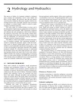
FIGURE 3.1 Algae were the rst colonizers of this 25-ha constructed wetland cell near Carson City, Nevada.
© 2009 by Taylor & Francis Group, LLC
Treatment Wetland Vegetation 65
is not surprising that some families are well represented by
multiple obligate wetland species. Vascular plants including
wetland plants may also be categorized morphologically by
descriptors such as woody, herbaceous, annual, or perennial.
Woody species have stems or branches that do not contain
chlorophyll. Because these tissues are adapted to survive for
more than one year, they are typically more durable or woody
in texture. Herbaceous species have aboveground tissues that
are leafy and lled with chlorophyll-bearing cells that typi-
cally survive for only one growing season. Woody species
include shrubs that attain heights up to 2 or 3 m and trees that
generally are more than 3 m in height when mature.
Annual plant species survive for only one growing sea-
son and must be reestablished annually from seed. Perennial
plant species live for more than one year and typically propa-
gate each year from perennial root systems or from perennial
aboveground stems and branches. Nearly all woody plant
species are perennial, but herbaceous species may be annual
or perennial.
Four groups of aquatic macrophytes (Figure 3.2) can
be distinguished on a basis of morphology and physiology
(Wetzel, 2001):
1. Emergent macrophytes grow on water-saturated

or submersed soils from where the water table is
about 0.5 m below the soil surface to where the
sediment is covered with approximately 1.5 m
of water (e.g., Acorus calamus, Carex rostrata,
Phragmites australis, Schoenoplectus (Scirpus)
lacustris, Typha latifolia).
2. Floating-leaved macrophytes are rooted in sub-
mersed sediments in water depths of approxi-
mately 0.5 to 3 m and possess either oating or
slightly aerial leaves (e.g., Nymphaea odorata,
Nuphar luteum).
3. Submersed macrophytes occur at all depths within
the photic zone. Vascular angiosperms (e.g., Myri-
ophyllum spicatum, Ceratophyllum demersum)
occur only to about 10 m (1 atm hydrostatic pres-
sure) of water depth and nonvascular macroalgae
occur to the lower limit of the photic zone (up to
200 m, e.g., Rhodophyceae).
4. Freely oating macrophytes are not rooted to the
substratum; they oat freely on or in the water and
are usually restricted to nonturbulent, protected
areas (e.g., Lemna minor, Spirodella polyrhiza,
Eichhornia crassipes).
In addition, a large number of the emergent macrophytes can
be established in oating mats, either with or without a sup-
porting structure. Some species have one or more of these
growth forms; however, there is usually a dominant form that
enables the plant species to be classied. In emergent plant
species, most of the aboveground part of the plant emerges
above the water line and into the air.

Both oating and submerged vascular plant species may
also occur in wetland treatment systems. Floating species have
leaves and stems buoyant enough to oat on the water surface.
Submerged species have buoyant stems and leaves that ll the
niche between the sediment surface and the top of the water
column. Floating and submerged species prefer deep aquatic
habitats, but they may occur in wetlands when water depth
exceeds the tolerance range for rooted, emergent species.
I. Emergent Aquatic Macrophytes
(a) (b) (c)
(d) (e) (f )
(g) (h)
(i) (j)
II. Floating Aquatic Macrophytes
III. Submerged Aquatic Macrophytes
FIGURE 3.2 Sketch showing the dominant life forms of aquatic
macrophytes. The species illustrated are (a) Scirpus (Schoeno-
plectus) lacustris, (b) Phragmites australis, (c) Typha latifolia, (d)
Nymphaea alba, (e) Potamogeton gramineus, (f) Hydrocotyle vul-
garis, (g) Eichhornia crassipes, (h) Lemna minor, (i) Potamogeton
crispus, (j) Littorella uniora. (From Brix and Schierup (1989b).
Ambio 18: 100–107. Reprinted with permission.)
© 2009 by Taylor & Francis Group, LLC
66 Treatment Wetlands
Table 3.1 lists the classes of plants reported in treatment
wetlands and their numbers. Table 3.2 lists the dominant
plants in treatment wetlands.
Adaptations to Life in Flooded Conditions
Prolonged ooding or waterlogging restricts oxygen move-
ment from the atmosphere to the soil. Diffusion can occur

but it is 10,000 times slower in saturated soils than it is in
aerated soils (Greenwood, 1961). Upon ooding, respiration
by aerobic bacteria and other organisms consume the oxy-
gen remaining in the soil within hours to days (Pezeshki,
1994). Soil oxygen deciency (partial hypoxia, complete
anoxia) poses the main ecological problem for plant growth
as it affects plant functions such as stomatal opening, photo-
synthesis, water and mineral uptake, and hormonal balance
(Kozlowski, 1984b). Life in permanently or periodically
anaerobic soils or substrates is more difcult than living in
mesic soils due to the nature of a highly reduced environment
(low redox potential), possibly together with soluble phyto-
toxins (Tiner, 1999).
A wide range of adaptations make it possible for plants to
grow in water or wetlands. These adaptations include physi-
ological responses, morphological adaptations, behavioral
re
sponses, reproductive strategies, and others (Table 3.3).
Major plant adaptations in free water surface (FWS) and
subsurface constructed wetlands are shown in Figures 3.3
and 3.4. For a detailed description of macrophyte adaptations
and responses to ooding see Hook and Crawford (1978),
Kozlowski (1984a), Crawford (1987), Hejný and Hroudová
(1987), or Jackson et al. (1990).
One of the most important adaptations to ooding is
the
development of aerenchymous plant tissues (Figure 3.5)
that transport gases to and from the roots through the vascu-
lar tissues of the plant above water and in contact with the
atmosphere, providing an aerated root zone and thus lower-

ing the plant’s reliance on external oxygen diffusion through
water and soil (Armstrong, 1978; Jackson and Drew, 1984;
Zimmerman, 1988; Brix, 1993). Lenticels or small openings
on the above water portions of these plants provide an entry
point for atmospheric oxygen into this aerenchymous tissue
network. Lenticel surface area may be increased through
plant growth, height increases, or the formation of swollen
buttresses in trees and woody herbs and in cypress knees.
Plant survival in ooded environments is a balance between
the severity of oxygen limitation and the adaptations available
to overcome this oxygen shortage. Thus, hydrophytic plants
may be adapted to survive and even grow in specic ooded
conditions, such as three months each year, or in “clean” or
owing water, which might have higher in situ dissolved oxy-
gen concentrations (Gosselink and Turner, 1978). However,
these same plants may not be able to grow or survive during
ve months of ooding or in stagnant or “dirty” water condi-
ti
ons. This is shown in Figure 3.3. Likewise, plants may have
adaptations that allow prolonged survival in one foot of water
but not at two feet. It may be hypothesized that this balance is
tilted unfavorably at higher water levels because of reduced
aerial plant stem surface area to provide oxygen to the roots
TABLE 3.1
Number of Plant Species by Group Found
in Constructed Wetlands in the North
American Database, Version 2.0*
Plant Group
Number of Species
Recorded

Emergent macrophyte 501
Floating aquatic plant 31
Submerged aquatic plant 10
Shrub 17
Tree 25
Unknown 5
Vine 5
Totals 594
*
This database is dominated by FWS wetlands, and cov-
ers only a subset of existing systems.
Source: Data from NADB database (1998) North Ameri-
can Treatment Wetland Database (NADB), Version 2.0.
Compiled by CH2M Hill, Gainesville, Florida.
TABLE 3.2
Dominant Plant Species Found in
Constructed Treatment Wetlands
Common Name Scientific Name
Bacopa Bacopa caroliniana
Bulrush Scirpus spp.
Cattail Typha spp.
Common reed Phragmites australis
Coontail Ceratophyllum demersum
Duck potato Sagittaria spp.
Duckweed Lemna spp.
Frogs-bit Limnobium spongea
Pennywort Hydrocotyle spp.
Pickerelweed Potederia spp.
Pondweed Potamogeton spp.
Reed canary grass Phalaris arundinacea

Softrush Juncus spp.
Spatterdock Nuphar luteum
Water hyacinth Eichhornia crassipes
Waterweed Elodea spp.
Source: Modied from NADB database (1998)
North American Treatment Wetland Database
(NADB), Version 2.0. Compiled by CH2M Hill,
Gainesville, Florida.
© 2009 by Taylor & Francis Group, LLC
Treatment Wetland Vegetation 67
through the lenticels and aerenchymous tissues. This proposed
explanation is supported by the nding that hydrophytes gen-
erally respond to ooding by growing taller, a growth response
that allows a more favorable balance between emergent and
submerged plant organs (Grace, 1989).
Hydropattern
The term hydropattern refers to the time series of water
depths in the wetland. The concept of hydropattern, or water
regime, includes two interdependent components: (1) the dura-
tion of ooded or saturated soil conditions (the hydroperiod
TABLE 3.3
Plant Adaptations or Responses to Flooding and Waterlogging
Morphological Stem hypertrophy (e.g., buttressed tree trunks); large air-lled cavities
Adaptations/responses In the center (stele) of roots and stems; aerenchyma tissue in roots and other plant parts; hollow stems;
shallow root systems; adventitious roots; pneumatophores (e.g., cypress knees); swollen, loosely
packed root nodules; lignication and suberization (thickening) of roots; soil water roots; succulent
roots; aerial root-tips; hypertrophied (enlarged) lenticle; relatively pervious cambium (in woody
species); heterophylly (e.g., submerged versus emergent leaves on same plants); succulent leaves.
Physiological adaptations Transport of oxygen to roots from lenticles and/or leaves (as often evidenced by oxidized rhizospheres);
anaerobic respiration; increased ethylene production; reduction of nitrate to nitrous oxide and nitrogen

gas; malate production and accumulation; reoxidation of NADH; metabolic adaptations
Other adaptations/responses Seed germination under water; viviparous seeds; root regeneration responses (e.g., adventitious roots);
growth dormancy (during ooding); elongation of stem or petioles; root elongation; additional cell
wall structures in epidermis or cortex; root mycorhizzae near upper soil surface; expansion of
coleoptiles (in grasses); change in direction of root or stem growth (horizontal or upward); long lived
seeds; breaking of dormancy of stem buds (may produce multiple stems or trunks).
Source: From Tiner (1999) A Guide to Wetland Identication, Delineation, Classication, and Mapping. CRC Press, Boca Raton, Florida.
FIGURE 3.3 Plant adaptations to primary domestic wastewater stresses in FWS wetlands. (Adapted from Wallace and Knight (2006) Small-scale
constructed wetland treatment systems: Feasibility, design criteria, and O&M requirements. Final Report, Project 01-CTS-5, Water Environment
Research Foundation (WERF): Alexandria, Virginia. Reprinted with permission.)
O
2
O
2
Low BOD,
N, P
Greater root penetration
because sediment is
less reducing
High water
column DO
Maximum water level
is greater since
resistance to internal
O
2
transport is low
Plant growth and size
are limited by
lack of nutrients

Plant growth and size are
not limited by lack of
nutrients; much more plant
biomass is present
Low internal
carbon (BOD) cycling
Water column
conditions favor
submerged and
emergent aquatic
plants
Root hairs
Rhizome
Clean Water
(Oligotrophic) Situation
Root hairs
Preferential
rooting in
upper
sediment
zone
Rhizome
Wastewater Situation
High BOD,
N, P
Highly reduced
sediment
Low water
column DO
O

2
High internal
carbon (BOD) cycling
Water column
conditions favor
phytoplankton (algae)
Maximum
water level is
only about
1/2 of clean
water
application
Limited root
penetration
O
2
Highly reducing sediment results in greater O
2
loss at root tip.
Plant can support less biomass with its finite internal O
2
transport capacity. Rooting occurs preferentially in upper
sediment layer where O
2
losses are minimized.
Less reducing sediment means that O
2
losses at root tip are minimized. Plant
can support more root biomass with its
finite internal O

2
transport capacity.
Plants grow deep to access nutrients.
© 2009 by Taylor & Francis Group, LLC
68 Treatment Wetlands
as a percentage of time with ooding), and (2) the depth of
ooding (Gunderson, 1989). Although hydroperiod refers
to the duration of ooding, the term water regime refers to
hydroperiod as well as to the combination of water depth
and ooding duration (depth-duration curve). The duration
and depth of ooding affect plant physiology because of soil
oxygen concentration, soil pH, dissolved and chelated macro
and micronutrients, and toxic chemical concentrations.
Figure 3.6 uses a graph of water level within a wetland over
an annual period to illustrate these two aspects of hydrope-
riod and water regime. Duration of ooding refers to the per-
centage of time that a wetland site is ooded or saturated,
and depth of ooding refers to the minimum, average, and
maximum depths of water at a given or typical spot within
40 um
(a)
20 mm
(b)
FIGURE 3.5 (a) Internal gas passages in a Phragmites root. (From Armstrong and Armstrong (1990b) In Constructed Wetlands in Water
Pollution Control. Cooper and Findlater (Eds.), Pergamon Press, Oxford, United Kingdom, pp. 529–534. Reprinted with permission.) (b)
Internal gas passages in a Typha culm.
FIGURE 3.4 Plant adaptations to primary domestic wastewater stresses in HSSF wetlands. (Adapted from Wallace and Knight (2006)
Small-scale constructed wetland treatment systems: Feasibility, design criteria, and O&M requirements. Final Report, Project 01-CTS-5,
Water Environment Research Foundation (WERF): Alexandria, Virginia. Reprinted with permission.)
High BOD,

N, P
Low BOD,
N, P
Limited root
penetration
Strongly reducing
conditions in
gravel bed
Wastewater Situation
Clean Water Situation
Preferential flow path at the
bottom of bed often develops.
Root hairs
Water level
Liner
No limitations
on root penetration
Mulch/detritus
layer
Root hairs
Rhizome
Rhizome
Preferential
rooting zone
Plant growth
and size are
limited by
lack of nutrients
Plant growth and size
not limited by lack of

nutrients; much more
biomass is present.
Highly reducing conditions result in greater O
2
loss at root tip.
Plant will support less root biomass because of its finite internal
O
2
transport capacity. Rooting occurs preferentially in upper bed
layer where O
2
losses are minimized.
Less reducing conditions in bed media
means that O
2
losses at root tip are
minimized. Plant can support more root
biomass with its finite internal O
2
transport
capacity. Roots can penetrate the full
depth of bed media.
© 2009 by Taylor & Francis Group, LLC
Treatment Wetland Vegetation 69
a wetland. Hydroperiod curves provide a convenient method
for estimating the percentage of time that a wetland is ooded
at any water depth and can summarize water level data over
any period of record. Note that water level charts and depth-
duration curves also can summarize the time and depth that
water is located below the ground surface.

Although the presence of water separates uplands from
wetlands and aquatic ecosystems, hydropattern is the most
important contributor to wetland type or class (Gosselink
and Turner, 1978; Gunderson, 1989). The importance of this
factor in wetland treatment system design and operation can-
not be overstated because incorrect understanding of the
hydroperiod and water regime limitations of wetland plant
species is a frequent cause of vegetation problems in natu-
ral and constructed wetlands. Measuring the hydroperiod is
relatively easy. However, selecting the optimal hydroperiod
for wetland treatment design and performance is complex.
OXYGEN TRANSPORT AS A TREATMENT FUNCTION
In order to survive in the saturated rooting environment,
emergent wetland plants transport oxygen from their leaves
down through their stalks to the root tissue (Armstrong, 1979).
Because the aerenchyma passageways have occasional block-
ages to prevent ooding if the root tissues are damaged, internal
transport of oxygen is a diffusion-limited process. Some plant
species can increase oxygen transport by convective ow of
gases (Brix, 1990; Armstrong and Armstrong, 1990a; Brix,
1994b). Dead and broken shoots and stubble also form air
pipes to the root zone. Of interest here is the fact that sig-
nicant quantities of oxygen pass down through the airways
to the roots (Brix and Schierup, 1990; Brix, 1993); and that
signicant quantities of other gasses, such as carbon dioxide
and methane, pass upward from the root zone. Internal gas
spaces in a Phragmites root and a Typha culm are shown in
Fi
gure 3.5.
The oxygen is used for root respiration and to help detoxify

the environment encountered by the growing root tip. Conse-
quently, there are limits as to how far plants can propagate their
root systems in a highly reducing environment (Armstrong
et al., 1990). Some—probably most—of the oxygen passing
down the plant into the root zone is used in plant respira-
tion (Brix, 1990). The excess supply of O
2
over that required
for plant respiration is termed the plant aeration ux (PAF),
has been the subject of many research endeavors (Armstrong
et al., 1990; Brix, 1990; Gries et al., 1990; Sorrell et al.,
2000; Wu et al., 2001; Bezbaruah and Zhang, 2003). The dif-
culty of measuring processes and concentrations in the root
microzones has been a major factor in the widely disparate
estimates of PAF (Kadlec and Knight, 1996).
Chemical conditions in the root zone are important deter-
minants of the potential for signicant PAF (Sorrell, 1999).
Hydroponic studies most often create root environments that
do not include a signicant sediment oxygen demand. Roots
are numerous under such conditions, and exchange oxygen
along much of their length (Armstrong et al., 1990). The
morphology and physiology of roots is very different in the
anaerobic environment often associated with treatment wet-
land soils. Under treatment conditions, the number of roots
is signicantly less than in clean soil or hydroponic condi-
tions. Roots become armored along much of their length, and
O
2
losses to the soil and water occur only in a small apical
region (Brix, 1994c).

Oxygen transfer by plants was initially thought to be a
dominant mechanism in SSF wetland treatment (Kickuth and
Könemann, 1987), but recent work has demonstrated that the
Water Depth
Time
JFMAMJJASOND
Flooded
Maximum water depth
Ground surface
Average water depth
–1
0
1
2
3
and
Depth Avg = 0.8 Max = 2.2
9
12
= 75%Hydroperiod =
FIGURE 3.6 Components of hydropattern: hydroperiod and wetland water regime. (From Kadlec and Knight (1996) Treatment
Wetlands. First Edition, CRC Press, Boca Raton, Florida.)
© 2009 by Taylor & Francis Group, LLC
70 Treatment Wetlands
vast majority of the oxygen transferred by the plant is used for
root metabolism, and the amount released to the rhizosphere
is small. Different test methods yield different results, but a
value of 0.02 g/m
2
·d has been established in two indepen-

dent studies (Brix and Schierup, 1990; Wu et al., 2001). As a
result, most modern designers have abandoned the concept of
plants acting as “solar powered aerators.” Since studies have
proven plant-induced oxygen transfer rates to be so small,
current design guidelines recommend assuming that oxygen
delivered to the wastewater by the plant roots is negligible
(U.S. EPA, 2000a). For a further discussion of root aeration,
see Chapter 5.
3.2 BIOMASS AND GROWTH
The term biomass is most frequently dened as the mass
of all living tissue at a given time in a given unit of Earth’s
surface (Lieth and Whittaker, 1975). It is commonly divided
into belowground (roots, rhizomes, tubers, etc.) and above-
ground biomass (all vegetative and reproductive parts above
the ground level). The term standing crop includes live parts
and dead parts of live plants that are still attached. These
dead parts of plants together with still standing dead plants
are called standing dead. The term litter refers to those dead
parts of the plant that have fallen on the ground or sediment,
but in some cases also includes standing dead. These com-
partments exchange material, but not uniformly, over the
course of the year (Figure 3.7).
Peak standing crop is dened as the single largest value of
plant material present during a year’s growth (Richardson and
Vymazal, 2001). In tropical communities, with an almost con-
stant biomass, it is not protable to search for an annual maxi-
mum (Westlake, 1969). However, in all other climatic regions
the biomass uctuates widely throughout the year (Dykyjová
and Kvet, 1978; Shew et al., 1981; Kaswadji et al., 1990). The
range of standing crop of wetland plants is quite large (Kvet,

1982; Mitsch and Gosselink, 1993; Vymazal, 1995). Another
terminology has been advanced by Mueleman et al. (2002),
which suggests that the total is phytomass, which is composed
of living material (biomass) and dead (necromass).
Gross Primary Production (also called Gross Primary
Productivity, or GPP) is normally dened as the assimilation
of organic matter by a plant community during a specied
period, including the amount used by plant respiration. Net
Primary Production, or NPP, is dened as the biomass that is
incorporated into a plant community during a specied time
interval, less that respired. This is the quantity that is mea-
sured by harvest methods and which has also been called net
assimilation or apparent photosynthesis. The term Net Aer-
ial (or Aboveground) Primary Production (NAPP) is dened
as the biomass incorporated into the aerial parts (leaf, stem,
seed, and associated organs) of the plant community (Milner
and Hughes, 1968).
NPP of freshwater marshes is estimated most frequently
through harvest of annual peak standing stocks of live and
dead plant biomass. When root biomass is measured, it is
usually an important part of net annual plant production.
Some researchers consider net primary productivity esti-
mates by peak standing stock to be underestimates because
they do not account for biomass turnover during the growing
season (Pickett et al., 1989). Kvet (1982) estimates turnover
rates (productivity/biomass) in the range of 1.1–1.5 for sub-
merged species, 1.05–1.5 for short emergent species, 1.05–
1.3 for tall emergent species, and 1.15 for tall graminoids. For
comparison, phytoplankton has a turnover rate in the range
o

f
450–600. Table 3.4 summarizes some typical estimated
net production data from wetland ecosystems, both natural
and treatment.
Q
o
Live
Live Dead
New soil
Litter
Standing
dead
Aboveground
Belowground
Phytomass
Water
Soil
T
L
D
a
U
e
Q
i
A
a
A
b
D

b
U
FIGURE 3.7 Transfers of materials in the biosphere of wetlands. Biomass consists of living, above and below ground components. Necro-
mass consists of dead roots and rhizomes, plus aboveground standing dead and litter. Phytomass is the combination of biomass and necro-
mass. Transfer to the phytomass occurs by external plant uptake (U
e
). Transfer back to surface water and porewater occurs via leaching (L)
and decomposition (D
a
and D
b
). Necromass residuals lose their identity, and accrete as new soils and sediments (A
a
and A
b
).
© 2009 by Taylor & Francis Group, LLC
Treatment Wetland Vegetation 71
Primary productivity of wetland plants is increased by
the availability of water, light, and nutrients. Adding waste-
water to wetlands generally increases the availability of water
and nutrients and consequently results in the stimulation
of gross and net primary productivity of these ecosystems
(Guntenspergen and Stearns, 1981; Nixon and Lee, 1986).
FERTILIZER RESPONSE
The growth of wetland plants, like that of terrestrial plants,
is stimulated by fertilization (Boyd, 1971; Jordan et al., 1999;
Mueleman et al., 2002). When a wetland becomes the recipi-
ent of waters with higher nutrient content than those it has
been experiencing, there is a response of the vegetation, both

in species composition and in total biomass. This response
has been detailed for the Houghton Lake wetland by Kadlec
and Alvord (1989). The increased availability of nutrients
produces more vegetation during the growing season, which
in turn means more litter during the nongrowing season. This
litter requires several years to decay, and hence the total pool
of living and dead material grows slowly over several years
to a new and higher value. A signicant quantity of structural
components are thus retained in the wetland.
Primary productivity of wetland plants is increased by
the availability of water, light, and nutrients. Adding waste-
water to wetlands generally increases the availability of
water and nutrients and consequently results in the stimula-
tion of gross and net primary productivity of these ecosys-
te
ms. Figure 3.8 illustrates the typical plant growth response
curve to increased concentrations of nitrogen and phospho-
rus. The maximum rate of plant growth is attained as nutri-
ent levels are initially increased. However, at higher nutrient
levels, plant growth levels off while luxury nutrient uptake
continues, and at higher nutrient concentrations, phytotoxic
responses are observed.
Figure 3.9 gives an example of this fertilizer response
for soft-stemmed bulrush, Schoenoplectus (Scirpus) validus,
grown in dairy wastewater. As the nitrogen concentration was
increased, both above- and belowground biomass increases
(Tanner, 1994). However, there is a suggestion of a maximum
TABLE 3.4
End of Season Plant Biomass in Wetlands
Species Location Reference Water S/P/E

Live Above
(g/m
2
)
Total Above
(g/m
2
)
Roots and
Rhizomes (g/m
2
)
Cattails
Typha latifolia Wisconsin Smith et al. (1988) N 105/245/290 — 1,400 450
Typha latifolia Texas Hill (1987) N 60/240/345 — 2,500 2,200
Typha glauca Iowa van der Valk and Davis (1978) N 120/265/290 2,000 — 1,340
Typha latifolia Michigan Unpublished data from
Houghton Lake
N 120/245/275 490 890 6,200
Typha latifolia Michigan Unpublished data from
Houghton Lake
S 120/245/275 1,240 2,310 2,900
Typha angustifolia Michigan Unpublished data from
Houghton Lake
S 120/245/275 1,886 3,615 —
Typha latifolia Kentucky Pullin and Hammer (1989) P — 5,602 — 3,817
Typha angustifolia Kentucky Pullin and Hammer (1989) P — 5,538 — 4,860
Bulrushes
Scirpus uviatilis Iowa van der Valk and Davis (1978) N 130/265/285 790 — 1,370
Scirpus validus* Iowa van der Valk and Davis (1978) N 120/210/300 2,100 — 1,520

Scirpus validus New Zealand Tanner (2001a) P 30/205/350 2,100 2,650 1,200
Scirpus validus Kentucky Pullin and Hammer (1989) P — — 2,355 7,376
Scirpus cyperinus Kentucky Pullin and Hammer (1989) P — — 3,247 12,495
Phragmites
Phragmites australis U.K. Mason and Bryant (1975) N 75/220/305 942 1,275 —
Phragmites australis Iowa van der Valk and Davis (1978) N — — 1,110 1,260
Phragmites australis Netherlands Mueleman et al. (2002) N 105/255/350 2,900 3,200 7,150
Phragmites australis Brisbane Greenway (2002) S — 1,460 2,520 1,180
Phragmites australis Netherlands Mueleman et al. (2002) P 105/255/355 5,000 5,500 3,890
Phragmites australis New York Peverly et al. (1993) L 100/270/330 10,800 — 8,700
Note: Water type is N  no wastewater, S  nutrients at secondary treatment levels, P  nutrients at primary treatment levels, L  landll leachate at around
300 gN/m
3
. S/P/E refers to the start, peak, and end yeardays of the growing season (add 182 days for Southern Hemisphere).
*
Currently known as Schoenoplectus tabernaemontani.
© 2009 by Taylor & Francis Group, LLC
72 Treatment Wetlands
at the highest concentrations. In fact, root death was noted
by Tanner (1994) in plants growing in piggery wastewaters,
where high ammonia concentrations (mean 222 mg/L) were
at potentially phytotoxic levels. For example, ammonia con-
centrations of 200 mg/L are known to be detrimental to water
hyacinths (de Casabianca-Chassany et al., 1992). Other stud-
ies have also established similar effects for other treatment
wetland plants. Hill et al. (1997) found dry matter production
of Typha latifolia, Phragmites australis, and Sagittaria lati-
folia were unaffected by ammonia in the concentration range
20–80 mg/L range. Dry matter production of Schoenoplec-
tus (Scirpus) acutus was found to be maximized in the 30–50

mg/L range, and then to rapidly fall off above 60 mg/L.
SEASONAL PATTERNS
The growth and senescence of the soft tissue macrophytes
commonly used for wastewater treatment all follow a com-
mon seasonal pattern in temperate climates. In northern
climates, growth begins at the time of frost disappearance
(around April), and senescence begins in early autumn
(around September). This autumnal decline creates standing
dead aboveground plant material, which subsequently in part
decomposes, and in part falls to the soil surface.
A specic case for Typha is shown in Figure 3.10, which
is representative of other emergent macrophytes as well.
New growth proceeds from small shoots that may be initi-
ated as early as late summer of the preceding year for Typha
(Bernard, 1999), but remain tiny and dormant over the
winter season. Aboveground biomass increases rapidly in
early spring, typically commencing from late February to
Late April, depending on climate. Growth tapers off, caus-
ing aboveground biomass to peak in late summer to early
autumn. The size of the peak standing crop varies consider-
ably with plant species and degree of nutrient availability (see
Table 3.4). Typically, there is some degree of senescence that
accompanies the later portions of the growth period, so that
the total peak standing crop exceeds the live peak standing
crop. During autumn, more rapid senescence occurs, leav-
ing only a residual of standing and/or prostrate aboveground
dead material.
Belowground biomass follows a much more muted
annual cycle. In some cases, available methods of root and
rhizome biomass measurement are not accurate enough to

clearly dene a pattern (Figure 3.10). In other cases, a mid-
summer depression has been found, to about 50% of the mid-
winter maximum (Smith et al., 1988; Mueleman et al., 2002).
But mid summer maxima were found for Sparganium and
Phragmites in Iowa (van der Valk and Davis, 1978). When
root biomass is measured, it is usually an important part of
net annual plant production. NPP estimates by peak stand-
ing stock are underestimates because they do not account for
biomass turnover during the growing season. For instance, a
multiplier of 1.2–1.4 for aboveground cattails and Spartina
has been reported by Cronk and Fennessy (2001).
In tropical or subtropical climates, seasonality is much
more muted (Figure 3.11). There may be periods of dormancy
0
0123
0.2
0.4
0.6
0.8
1
1.2
Nutrient Supply
Plant Biomass
Nutrient
limited
Optimal
growth
Nutrient
toxicity
FIGURE 3.8 General relationship between plant biomass and

nutrient concentration in the water column.
y = –0.2534x
2
+ 58.59x
R
2
= 0.8673
0
500
1,000
1,500
2,000
2,500
3,000
3,500
4,000
TKN (mg/L)
Total Biomass (g/m
2
)
0 20 40 60 80 100 120 140
FIGURE 3.9 Growth of Schoenoplectus (Scirpus) validus in dairy wastewater at various dilutions. The accompanying range of total phos-
phorus concentrations was 0.3–14.8 mg/L. (Data from Tanner (1994) Aquatic Botany 47(2): 131–153.)
© 2009 by Taylor & Francis Group, LLC
Treatment Wetland Vegetation 73
and of regrowth, but there is typically not complete senes-
cence and death of all aboveground plant parts.
Two other factors are important in assessing the growth
of wetland plants: the length of the growing season, and
belowground productivity. All of the growth for the year

occurs in about 100 days in high latitudes, whereas systems
in the tropics grow year-round (see Table 3.4). Therefore, the
instantaneous growing season rate is much higher than the
annualized rate for northern systems. Belowground biomass
is typically comparable to aboveground biomass, although
the root-to-shoot ratio is sensitive to nutrient status and other
variables. The ratio of below to aboveground biomass is gen-
erally less in a fertilized environment than in a lower nutrient
(natural) environment (Mueleman et al., 2002). Kadlec and
Alvord (1989) indicated that belowground biomass responded
to fertilization differently from aboveground biomass. The
initial vegetation showed greatly reduced root biomass in
response to the added nutrients: 1,500 g/m
2
versus 4,000
g/m
2
at the end of the growing season. There are some reports
that root growth and activity continues much longer than for
aboveground plant parts (Prentki et al., 1978).
Roots and rhizomes persist over winter in northern cli-
mates, and therefore standing crop alone is not a measure of
productivity. Estimates of turnover times are on the order of
two to three years for herbaceous wetland plants. For example,
Tanner (2001a) estimated a lifetime of 18 to 24 months for
Schoenoplectus rhizomes, and Prentki et al. (1978) reported
1.5–2 years for Typha rhizomes and at least three years for
Phragmites rhizomes. Therefore, the total growth rate for wet-
land plants is much higher than for aboveground parts alone.
These factors lead to the conclusion that plant growth is

much higher than one standing (aboveground) crop per year.
Table 3.5 presents a hypothetical illustration of factors for
two climate zones. The growth of plant biomass during the
0
500
1,000
1,500
2,000
2,500
3,000
0 90 180 270 360
Yearday
Phytomass (g/m
2
)
Aboveground
Belowground
FIGURE 3.10 Seasonal patterns of above- and belowground Typha angustifolia phytomass at Richardson, Texas. The climate is warm
temperate. Points are averages for two years. (Data from Hill (1987). Aquatic Botany 27: 387–394.)
0
10,000
20,000
30,000
40,000
50,000
0 90 180 270 360
Yearday
Phytomass (g/m
2
)

Total Belowground Aboveground
FIGURE 3.11 The pattern of growth of Phragmites australis in the warm dry continental climate of Grifth, Australia. The water phospho-
rus concentration was 12 mg/L, and the approximate annual temperature range was from 10–23°C. (Data from Hocking (1989a) Australian
Journal of Marine and Freshwater Research 40: 421–444.)
© 2009 by Taylor & Francis Group, LLC
74 Treatment Wetlands
respective growing seasons is about the same, but the growing
season is much attenuated in northern climates. As a result,
the annual growth is higher in the warmer environment.
Start-Up: Wetland Vegetation Changes
A constructed wetland begins its existence with the vegeta-
tion placed by the constructors, and the seed bank associated
with the selected soils. A natural wetland will have evolved
over time to contain a mix of vegetation commensurate with
the hydropattern and water quality conditions prior to waste-
water addition. In either case, the wetland vegetation is likely
to change over the course of time, as local adaptations to the
treatment hydropattern and quality occur. The plant commu-
nity that develops over time is a function of organic loading,
hydrology, and climate. FWS wetlands that are heavily loaded
with organic matter and nutrients will typically develop a less
diverse plant community since fewer plant species are able
to tolerate the reducing conditions that develop under these
circumstances. In polishing wetlands with very high water
quality, a diverse species composition may develop.
INDIVIDUAL PLANTS
Plants reproduce in a two principal ways, by seeding and by
vegetative reproduction. A plant starting from seed is a new
individual, whereas it is not so easy to identify new individu-
als when new shoots arise from underground runners. Bul-

rushes tend to spread in a radial habit, with clumps growing
in diameter. Cattails and Phragmites tend to spread in a lin-
ear mode, with new shoots emerging from a runner at inter-
vals (Figure 3.12). Such runners can extend several meters
in just one growing season, for both cattails and Phragmites.
Aboveground parts of plants in cold environments have
a life span dictated by the photoperiod and frost conditions
TABLE 3.5
Hypothetical Growth Characteristics of Wetlands Growing in Temperate and Subtropical Conditions
Characteristic Unit
Temperate Growing
Season (M–J–J–A) Annual Subtropical Annual
Peak standing crop aboveground g/m
2
2,000 2,000 2,000
Growth (GPP/NPP  1.3)
g/m
2
2,600 2,600 —
Growth (4 turnovers per year) g/m
2
— — 8,000
Growing season days 120 365 365
Growth rate above g/m
2
·d 21.7 7.1 21.9
Belowground crop (root/shoot  1.0)
g/m
2
2,000 2,000 2,000

Growth (0.5 turnovers per year) g/m
2
1,000 1,000 1,000
Growing season days 240 365 365
Growth rate below g/m
2
·d 4.2 2.7 2.7
Total growth rate g/m
2
·d 25.8 9.9 24.7
Annualized instantaneous growth rate g/m
2
·yr 9,429 3,600 9,000
Undepleted solar radiation MJ/m
2
·d 38 24 31
Note: These both grow at about the same rate during their respective growing seasons, which are year round in the warm climate.
of the region. They live through one growing season, and
new plants emerge the next year, from root stock or from
seed. However, in warm climates, individual plants may
persist for more than one year. Davis (1989) tagged indi-
vidual leaves of 43 individual shoots of Typha domingensis,
and followed their growth over their entire life history in a
F
l
orida wetland (Figure 3.13). He found that leaf growth and
mortality continued throughout the life span of each tagged
plant. New leaves emerged and grew, even while total bio-
mass declined. Older leaves senesced, broke, or died even
while total biomass increased. This continual growth and

mortality resulted in an annual turnover of 4.4 ± 0.7 times
the mean standing crop (Davis, 1989).
The concept of individual plant life history becomes
important when, as is a common case, an entire wetland is
planted at one time, creating a cohort of plants that will all
live about the same length of time. Clearly, without regenera-
tion this wetland will be devoid of plants after a few years.
Therefore, the key to a self-sustaining wetland plant com-
munity is not only the survivability of plants in the treatment
environment, but also the ability to regenerate.
PLANT COVERAGE
The vegetative cover of a treatment wetland refers to the area
of wetland plants, and is concerned with four principal mea-
sures: (1) fraction areal coverage, (2) stem density, (3) sub-
merged area, and (4) underwater porosity.
Fra
ctional Coverage
Most FWS constructed treatment wetlands are not mono-
typic communities, but rather contain a patchwork of open
water, SAV, EAV, and FAV. In contrast, many SSF systems
are in fact completely vegetated with uniform stands of EAV.
© 2009 by Taylor & Francis Group, LLC
Treatment Wetland Vegetation 75
In both cases, the vegetation contributes to treatment, with
greater effect at lighter pollutant loadings. For example, FWS
phosphorus removal has been strongly linked to the fractional
coverage of different community types (Lakhsman, 1982;
Juston, 2006). Therefore, it is useful to distinguish between
various degrees of vegetative completeness. Aerial photogra-
phy or other remote sensing can be used to measure coverage

of emergent plants, but it is more difcult to determine the
presence of SAV (Rutchey and Vilcheck, 1999). If the wetland
has design bathymetry including deep zones, then that infor-
mation provides estimates of coverage of EAV.
FIGURE 3.12 Phragmites spreads vegetatively via linear runners. Dr. Hans Brix holds a specimen of only a few weeks’ age, in a sludge
drying reed bed in Denmark.
Stem Density
The stem density of wetland plants is important because the
resistance to water ow is determined in part by stem density.
Only a small fraction of the ultimate plant density is planted in a
new wetland. Planting densities range from 1,000–40,000 plants
per hectare (0.1–4.0 plants per m
2
), depending on the rate of
spread of the selected plant species and the acceptable timeframe
for plant establishment. Through vegetative reproduction, these
plants will eventually spread to much greater densities.
Tanner reported 1,400–1,500 stems per m
2
for Schoeno-
plectus tabernaemontani growing in dairy wastewater (Tan-
ner, 2001a), and over 2,000 stems per m
2
for Schoenoplectus
validus (Tanner, 1994). In contrast, stem counts for Scirpus
acutus in the Sacramento, California, project were typically
only 150 per m
2
in secondary efuent, although accompanied
in some cases by 15–30 per m

2
Typha latifolia plants (Nolte
and Associates, 1997; 1998a).
Cattails generally have many fewer stems per unit area
than bulrushes. For instance, the discharge area at Houghton
Lake, Michigan, had 71 ± 23 per m
2
for Typha latifolia, and 89
± 22 per m
2
for Typha angustifolia. A nutrient-poor location at
the same wetland had only 35 ± 22 per m
2
for Typha latifolia.
Glenn et al. (1995) measured 140 per m
2
for Typha domin-
gensis in northern Mexico. Phragmites australis has compa-
rable numbers in secondary reedbeds, 70–100 per m
2
in the
United Kingdom (Daniels and Parr, 1990; as referenced by
Cooper et al., 1996). However, Phragmites australis grows
to higher densities in warm climates, around 250 per m
2
in
Australia (Hocking, 1989a).
Hydraulic modeling has therefore adopted similar stem
density numbers. For instance, Nepf et al. (1997) used stem
(cylinders) densities of 200–2,000 per m

2
in constructed
ume experiments, to represent Juncus roemerianus. Hall
and Freeman (1994) studied hydraulics in constructed umes,
0
10
20
30
40
50
60
70
80
90
0122436
Months from December 1974
Aboveground Biomass (g)
Unimodal
Bimodal
FIGURE 3.13 Growth of single shoots of Typha domingensis in a
subtropical wetland. (Data from Davis (1989) Sawgrass and cattail
production in relation to nutrient supply in the Everglades. Sharitz
and Gibbons (Eds.). U.S. Department of Energy Conference No.
8603101, held in Charleston, South Carolina; National Technical
Information Service: Springeld, Virginia, pp. 325–341.)
© 2009 by Taylor & Francis Group, LLC
76 Treatment Wetlands
with bulrush plants, at densities of 400 and 800 per m
2
. In

laboratory umes, Schmid et al. (2004b) used 12.8 stems
(cylinders) per m
2
as representative of Typha latifolia.
Submerged Area
Since microbial transformations within a FWS wetland are
largely a function of area available for biolm growth, the cre-
ation of surface area by emergent aquatic plants and associated
leaf litter is an important contribution to the treatment process.
One method to assess the relative contribution of the plants is
to measure the amount of submerged surface area available
per area of wetland (submerged specic surface area). For
instance, a waste stabilization pond would have a specic sur-
face area of 1.0 m
2
/m
2
as the only wetted surface area is the
bottom of the pond. Specic surface areas for wetlands are
higher, averaging 2.8 m
2
/m
2
at depth 30 cm for various spe-
cies (Table 3.6). The depth dependence of specic surface is
nearly linear (U.S. EPA, 1999).
The reader is cautioned that submerged area differs mark-
edly from the leaf area index (LAI), the latter being com-
monly used in studies of photosynthesis and transpiration.
LAI measures the total area of leaves in the air above water.

Under most normal depths of operation, the large majority
of leaf area will be above water. For instance, Scirpus leaves
were measured to have LAI of 5.3–6.5 m
2
/m
2
, and Typha of
4.1–5.5 m
2
/m
2
at the Sacramento, California wetlands (Nolte
and Associates, 1998a).
Underwater Porosity
The actual detention time in a FWS wetland is the wetland
water volume divided by the volumetric ow rate. In turn,
the actual water volume is less than the bathymetric value,
because submerged stems take up space. The literature con-
tains pronouncements of appropriate estimates ranging from
0.65 (Reed et al., 1995) to 0.95 (Kadlec and Knight, 1996).
Porosity depends upon stem density and stem size. For cylin-
drical stems, the relationship is:
EH
P
1
4
2
D
(3.2)
where

D  stem diameter, m
E = porosity fraction
H = stem density, no. per m
2
For instance, at the Houghton Lake, Michigan, site, there
were 96 Typha latifolia stems per m
2
, and the mean stem
diameter in the 30 cm depth was 1.2 cm. The cylinder poros-
ity was therefore 99%. As may be conrmed from Equation
3.2, it is only when there are large numbers of stems of large
diameter that porosity drops below 95%, for example, more
than 100 per m
2
at diameter 2.5 cm. Such extreme sizes and
densities are uncommon, but may be encountered in warm
climates. For instance, Hocking (1989a; 1989b) reports stem
densities of 250 per m
2
, and basal diameters of one cm may
be inferred from his data for Phragmites australis in a nutri-
ent-rich warm climate. The corresponding cylindrical poros-
ity is 96%.
In many circumstances in FWS, topographical “block-
age” is more important than vegetative wet volume exclusion
(see Chapter 2).
Root Penetration
Early literature on HSSF wetlands contained much emphasis
on the importance of root penetration depth and its effect on
treatment (U.S. EPA, 1993f; Reed et al., 1995). The percep-

tion was that some wetland plants would have greater rooting
depths, and hence provide more radial oxygen loss to con-
duct aerobic processes in the rhizosphere. It is indeed true
that plants differ in their rooting proles in relatively clean
water, but it is now known that rooting proles do not differ
much among species in nutrient-rich waters (see Chapter 2,
Fi
gure 2.29). Roots are predominantly in the upper 20–30 cm
of the media in both HSSF and FWS wetlands.
3.3 LITTERFALL AND DECOMPOSITION
Over the life cycle of a vascular plant, all plant tissues are
either consumed, exported, or eventually recycled back to
the ground as plant litter. Litterfall and the resulting decom-
position of organic plant material are ecologically important
functions in wetlands, and contribute to the cycling of nutri-
ents and pollutants.
LITTERFALL
Wetland plant tissues fall at variable rates depending on the
survival strategy of the individual plant species. Herbaceous
TABLE 3.6
Submerged Surface Area in Ponds, and Wetlands
at Depth 30 cm
Treatment System Vegetation
Submerged
Area (m
2
/m
2
)
Waste stabilization pond None

1.0
Water hyacinth pond Eichhornia crassipes
2.2
Arcata, California Scirpus acutus
4.5
Arcata, California Typha latifolia
2.0
Benton, Kentucky Scirpus cyperinus
3.1
Benton, Kentucky Typha latifolia
2.1
Houghton Lake, Michigan Typha latifolia
2.1
Houghton Lake, Michigan Typha angustifolia
2.7
Pembroke, Kentucky Scirpus validus
2.7
Pembroke, Kentucky Typha angustifolia
3.2
Note: Litter and basin side walls are excluded.
Source: Data from U.S. EPA (1999) Free water surface wetlands for
wastewater treatment: A technology assessment. EPA 832/R 99/002,
U.S. EPA Ofce of Water: Washington D.C. 165 pp.; and Khatiwada
and Polprasert (1999a) Water Science and Technology, 40(3): 83–89.
© 2009 by Taylor & Francis Group, LLC
Treatment Wetland Vegetation 77
plant species typically recycle the entire aboveground
portion of the plant annually in temperate environments.
The growth season may vary from ten or more months in
subtropical regions to less than three months in colder cli-

mates. Also, most herbaceous species lose a fraction of liv-
ing leaf and stem material as litter throughout the growing
season, so there is a continuous rain of dead plant tissues
throughout the year with seasonal highs and lows of litter-
fall. Woody plant species also participate in this production
of plant litter through a natural pruning of small branches
throughout the annual period. In the northern hemisphere,
large amounts of owers are shed during the spring, and
leaves and fruiting bodies are lost during the fall.
Most herbaceous wetland plants do not directly fall to
the wetland oor after senescence and death. Instead, plants
remain in an upright stance until meteorological conditions
cause them to topple. Wind, rain, and especially weight of
snow, cause the standing dead material to fall. Terminol-
ogy varies, and so dead material is sometimes called litter,
regardless of whether it is upright or not. At other times, a
distinction is drawn between standing dead and prone mate-
rial called litter.
DECOMPOSITION
Decomposition generally refers to the disintegration of dead
organisms into particulate form (or detritus), and the further
breakdown of large particles to smaller and smaller particles,
until the structure can no longer be recognized and complex
organic molecules have been broken down into CO
2
, H
2
O,
and mineral components (Mason, 1977). In wetland studies,
the term decomposition is mostly conned to the breakdown

and subsequent decay of dominant macrophytes, which leads
to the production of detritus. Most net annual aboveground
production of wetlands is not consumed by herbivores but
decomposes on the wetland surface. Rates of decomposi-
tion vary in wetlands and the fate of materials released and
adsorbed during decomposition depends on the physical and
chemical composition of material as well as environmental
conditions at the site of decomposition (Vymazal, 1995).
Studies of litter decomposition are very numerous in the
literature. Techniques for such studies have been compiled
in books (Barlocher et al., 2005). Most of these studies have
been concerned with aboveground plant parts.
The decomposition of litter and resultant release of nutri-
ents involve at least two processes (Godshalk and Wetzel,
1978a) An initial loss of soluble materials is attributed to
abiotic leaching (Boyd, 1970; Gosselink and Kirby, 1974;
Godshalk and Wetzel, 1978b; 1978c; 1978d). This process
is quite rapid and accounts for the majority of mass reduc-
tion during the early stages of decomposition. Leaching
occurs very quickly under both aerobic and anaerobic con-
ditions with most of the water-soluble organic substances
being released within a few days. The rapid initial release of
nutrients by leaching has been documented in many marsh
plants—up to 30% of nutrients are lost by leaching alone
during the rst few days of decomposition (Vymazal, 1995).
In submerged and oating-leaved plants, leaching accounts
for up to 50% loss of dry matter within the rst two to three
days. Released nutrients may be incorporated into the pro-
toplasm of decomposer organisms where activities such as
respiration and denitrication account for additional nutrient

losses (Mason and Bryant, 1975).
Flooding in wetlands has been found to increase the lit-
ter decomposition rate through physical leaching of inorganic
and organic compounds from the plant tissues (Day, 1989;
Whigham et al., 1989) and by providing habitat for aquatic
microbes and invertebrates, which are important mediators in
this process. However, if ood waters are anaerobic, biological
activity is greatly reduced (Tupacz and Day, 1990) and only the
leaching mechanisms and anaerobic respiration will occur.
PATTERNS OF WEIGHT LOSS
Chemical analysis of plant material reveals different rates of
decomposition for different components of the plant material
(soluble components, cellulose, hemicellulose, and lignin),
and that rates of decomposition of each component change
over time, such that the specic rate of decay for each fraction
decreases as decomposition proceeds (Moran et al., 1989).
The initial sharp drop in necromass is followed by a decline
to an undecomposed residual. The initial drop is typically of
the order of 10–20% for soft-tissue emergent macrophytes
(Table 3.7).
The residual of recalcitrant substances is on the order of
5–20%, as inferred from long-term accretion studies. Rarely
are decomposition studies continued to the point where such
residuals can be determined. This is in major part due to the
length of time required, as well as to the limitations of mea-
surement techniques. An example of a litter residual is shown
in Figure 3.14.
When these features are considered in combination, a
modied rst-order loss equation results:
MM

MM
Akt


¤
¦
¥
³
µ
´

*
*
exp( )
o
(3.3)
where
A = fraction remaining after initial leaching
k = mass loss rate coefcient, d
-1
M
o
= initial mass, g
M = mass remaining, g
M
*
= residual mass remaining, g
t = time, d
In the vast majority of literature studies, the value of M* is
chosen to be zero; and the value of A is selected to be unity.

There is then only one parameter to consider, the lumped
mass loss rate coefcient, and under these special circum-
stances, it is here denoted by k
1
. Chimney and Pietro (2006)
provide rates of litter decomposition of 140 different wet-
land plant varieties (Table 3.8). Mean rst-order rate coef-
cients (k
1
) for emergent macrophyte leaf litter decomposition
© 2009 by Taylor & Francis Group, LLC
78 Treatment Wetlands
TABLE 3.7
Initial Weight Loss for Submerged Litter in
Treatment Wetlands
Site Wetland Water Typha Scirpus Data Source
Sacramento,
California
Nolte and
Associates
(1998a)
1A WW 0.01 0.03
1B WW 0.15 0.35
7A WW 0.03 0.90
7B WW 0.21 0.56
9A WW 0.00 0.82
9B WW 0.17 0.14
Mean WW 0.10 0.47
Sacramento,
California

Nolte and
Associates
(1998a)
5A Control 0.14 0.00
5B Control 0.00 0.00
LC3 Control 0.15 0.10
LC4 Control 0.18 0.16
Mean Control 0.12 0.07
Léon, Spain Alvarez and
Becares
(2006)
Winter WW 0.14 —
Summer WW 0.15 —
Theresa Marsh,
Wisconsin
Puriveth
(1980)
— Runoff 0.09 0.11
Houghton Lake,
Michigan
Kadlec
(1989)
— WW 0.14 —
— Control 0.06 —
Note: WW = wastewater; values were determined by data tting.
averaged 1.4 yr
−1
for 32 studies of Phragmites australis,
1.7 yr
−1

for 23 studies of 10 Scirpus species, and 1.4 ± 0.9 for
72 studies of 8 Typha species. Variability for a single plant
across studies is not great (Table 3.9). The half-life of the lit-
ter is equal to 0.693/k
1
.
Litter decomposition is largely mediated by vertebrates,
invertebrates, and microbes living in wetlands. New litter is
typically conditioned by fungi and bacteria before it is shred into
smaller particles by aquatic macroinvertebrates (Merritt and
Lawson, 1979). The activity of these organisms is condi-
tioned by temperature, and therefore a temperature effect
on decomposition is to be expected. Studies by Alvarez and
Becares (2006) conrm this effect, as a differential in rates
in summer and winter (Table 3.9). It is also true that warmer
climates show higher rates of litter decomposition on an
0
20
40
60
80
100
0 30 60 90 120 150 180 210 240 270 300
Time (days)
Percent Remaining
Control
Treatment
k-C* model
FIGURE 3.14 Leaf litter decomposition in treatment and control
wetlands at Thibodeaux, Louisiana. Species were Fraxinus penn-

sylvanica, Salix nigra, Taxodium distichum, Nyssa aquatica, and
Acer rubrum. Two outliers removed for modeling. (Data from
Rybczyk et al. (2002) Wetlands 22(1): 18–32.)
TABLE 3.8
Summary of Lumped Loss Rate Coefficients for
Herbaceous Plants in Various Wetlands
Species
Data Sets
N
Mean k
1
(yr
−1
)
Median k
1
(yr
−1
)
Mean
Half-Life
(d
−1
)
All
submersed
species
107 17.3 10.2 15
All oating
species

80 13.9 8.9 18
All emergent
species
280 3.03 0.80 83
TABLE 3.9
Values of the Lumped Loss Rate Coefficients for
Typha in Various Treatment Wetlands
Species Location
Mean k
1
(yr
−1
)
Half-Life
(d
−1
)
Typha wastewater Sacramento, California 0.71 356
Typha control Sacramento, California 0.82 308
Typha wastewater,
summer
Leon, Spain 1.57 161
Typha wastewater,
winter
Leon, Spain 0.73 347
Typha wastewater,
average
Leon, Spain 1.15 220
Typha runoff Theresa Marsh, Wisconsin 0.70 361
Typha wastewater Houghton Lake, Michigan 0.50 506

Typha control Houghton Lake, Michigan 0.71 356
Typha runoff ENRP, Florida 1.72 147
© 2009 by Taylor & Francis Group, LLC
Treatment Wetland Vegetation 79
annual basis. However, the effect of frozen winter conditions
typically interrupts the decay processes, which effectively
come to a halt in frozen water and soils (Figure 3.15). There-
fore, part of the variability across data sets has to do with this
winter-season shutdown.
COMBINED EFFECTS OF SUCCESSIVE COHORTS
Research has in general focused on the fate of a particular
cohort of necromass, placed in a porous bag and isolated
from other materials in the wetland. However, the litter layer
in the wetland is the result of many such cohorts that accrue
over the years, and the decomposition processes that reduce
each of them over time. A conceptual model of this suc-
cessive accrual and decomposition is shown in Figure 3.16,
for the case of startup of a new wetland. As a simple exam-
ple, consider litter which has a half-life of one year, being
deposited once per year in cold temperate climate. At the end
of year one, a fresh “crop” of litter of mass M
o
is present. At
the end of year two, half that remains, and another crop of M
o
is added, with the total now being 1.5 M
o
. A bit of arithmetic
shows that, after a period of some years, this process will
lead to an end-of-season litter crop that is twice the annual

litterfall. It will take ve years to build the litter to 97% of
the nal value. Of course, events are not so simple in a real
situation, but this conceptual model serves to illustrate that a
wetland has considerable “memory” via the process of litter
accumulation and decomposition.
BELOWGROUND DECOMPOSITION
Roots and rhizomes also undergo mortality and decomposi-
tion. Asaeda and Nam (2002) found a mean half-life of 1.2
years for Phragmites rhizomes of age greater than one year.
Hill (1987) found 1.84 years for below ground cattail (Typha
angustifolia). Sharma and Gopal (1982) reported 75% loss
of Typha elephantina rhizomes decomposed in six months,
in India (half-life 0.25 years). Tanner (2001a) found 1.5–2.0
years half-life for rhizomes of soft stem bulrush (Schoeno-
plectus tabernaemontani). Prentki et al. (1978) reported
1.5–2 years for Typha rhizomes and at least three years for
Phragmites rhizomes. The fraction of this necromass which
contributes to below ground soil accretion has not been deter-
mined. It seems probable that most root-rhizome necromass
is recycled and only a small fraction ultimately contributes
to an underground residual soil accretion. However, the rates
of decomposition are slower than for aboveground litter, and
therefore the belowground litter crop is much more than dou-
ble the annual belowground production. It also takes much
longer for the belowground litter standing crop to develop.
THATCH
In especially hot and arid climates, treatment wetlands
can accumulate excessive quantities of dead plant biomass,
0.0
0.2

0.4
0.6
0.8
1.0
0 365 730 1095
Time (days)
Fraction Remaining
Control
Pipeline
Frozen conditions
FIGURE 3.15 Decomposition of cattail (Typha spp.) litter in wastewater and control areas of the Houghton Lake, Michigan, wetland. Material
was placed on September 2. Freeze-up occurs around November 1, and thaw around May 1. No weight loss occurred during frozen conditions.
0.0
0.2
0.4
0.6
0.8
1.0
1.2
1.4
1.6
1.8
2.0
012345
Year
Relative Amount of Litter
Year 5
Year 4
Year 3
Year 2

Year 1
FIGURE 3.16 Cohorts of litter accumulate and decompose during
the course of time. (From Rybczyk et al. (2002) Wetlands 22(1):
18–32. Reprinted with permission.)
© 2009 by Taylor & Francis Group, LLC
80 Treatment Wetlands
regionally referred to as thatch. This accumulation results
from the low decomposition rates occasioned by lack of
water to support decomposer organisms, plus the upright
orientation of the necromass, which keeps the material in
the air rather than in the water. The high productivity of
the litter, coupled with slow decomposition, leads to very
large standing crops of standing dead thatch (Figure 3.17).
Mechanical harvesting may be used to remove standing dead
aboveground material (combing or thinning) or both dead
above- and belowground (thatching) (Nolte and Associates,
1998b; Thullen et al., 2002). Controlled burning is one alter-
native to remove excess plant biomass in wetland treatment
systems, although ash produced by burning will reintroduce
nutrients into the water column. This can potentially cause
a short-term decrease in treatment efciency. Burning has
been implemented at sites that permit such activities. Since
accumulated plant necromass can regenerate, the benets of
removal are only temporary (Thullen et al., 2002).
In contrast, in cold climates the presence of standing dead
material provides an excellent adjunct to insulation. Firstly,
the standing material protects the wetland soil or water
surface from direct exposure to the wind. This wind-break
function is probably secondary to the function of catching
snow, often to a depth of a meter or more. Snow is held up

on dead plants, creating a zone of air spaces interlaced with
plant material and captured snow (Figure 3.18). This com-
posite is an excellent thermal insulator, and often prevents
freezing in vegetated natural wetlands at times when water
is deeply frozen. This function is served for both FWS and
HSSF wetlands.
The litter layer on top of a HSSF wetland bed functions
as mulch. Such a layer also provides air spaces and holds up
the snow to form an insulating layer for the SSF bed.
MINERAL CONSTITUENTS OF LITTER
The chemical composition of litter is not xed during decom-
position. Carbon and macronutrients (N, P, Ca, K) may be
depleted or amplied at differential rates. Decomposer
FIGURE 3.17 Thatch at the Tres Rios Hayeld wetland near Phoenix, Arizona. This standing dead material is over two meters in height,
and has totally blocked light penetration to the wetland water.
FIGURE 3.18 Standing dead wetland plants capture snow and pro-
vide thermal insulation.
© 2009 by Taylor & Francis Group, LLC
Treatment Wetland Vegetation 81
organisms utilize chemicals from both water and the litter,
and then contribute to the overall biomass of the litter. For
example, the rate of concentration increase may exceed the
rate of necromass loss, thereby creating an increase in the
mass of a constituent (Figure 3.19). The additional chemicals
are acquired from the wetland water. In other situations, there
can be a mass loss of chemicals accompanying the loss of
necromass (see, for instance Kulshreshtha and Gopal, 1982;
Corstanje et al., 2006). There appears to be no universal pat-
tern for the time series of litter chemical composition in natu-
ral or treatment wetlands (Chimney and Pietro, 2006).

ACCRETION
Wetland ecosystems are often sites of long-term positive net
primary productivity (NPP), and develop accumulations of
buried organic matter in the form of peat and eventually coal.
This net accumulation of organic matter is primarily because
of the reduced metabolic rate of microbes in ooded wet-
land sediments compared to metabolic rates in well aerated,
upland soils. When living and dead plant material sinks to
the level of anaerobic sediments, it is protected from abun-
dant free oxygen and from the higher rates of degradation
typical of an oxygenated system.
Therefore, not all of the dead plant material undergoes
decomposition. Some small portions of both aboveground
and belowground necromass resist decay, and form stable
new accretions. The amount of such accretion has been quan-
tied in only a few instances for free water surface wetlands
(Craft and Richardson, 1993; Reddy et al., 1993; Rybczyk
et al., 2002), although anecdotal reports also exist (Kadlec,
1997a; Sees, 2005; Wang et al., 2006a). Quantitative stud-
ies have relied upon either atmospheric deposition markers
(radioactive cesium or radioactive lead) or introduced hori-
zon markers, such as feldspar or plaster. Either technique
requires several years of continued deposition for accuracy.
The manner of accretion has sometimes been presumed
to be sequential vertical layering (Kadlec and Walker, 1999;
Rybczyk et al., 2002), but that view is likely to be overly sim-
plied. At least two factors argue against simple layering:
0
20
40

60
80
100
0 3 6 9 12 15 18 21 24
Time (months)
Percent Remaining
(a)
0.0
0.5
1.0
1.5
2.0
0 3 6.5 8.5 12 15 18 24
Time (months)
Percent N
0.000
0.025
0.050
0.075
0.100
Percent P
Nitrogen
Phosphorus
(b)
FIGURE 3.19 Changes in amount of culm litter (a), nitrogen (N), and phosphorus (P) content (b), and N&P stock (c) for Phragmites over a
two-year period of decomposition. (From Gessner (2000). Aquatic Botany 66(1): 9–20. Reprinted with permission.)
0
50
100
150

200
250
300
350
0 3 6.5 8.5 12 15 18 24
Time (months)
Percent N Stock
0
50
100
150
200
250
300
350
Percent P Stock
Nitrogen
Phosphorus
(c)
© 2009 by Taylor & Francis Group, LLC
82 Treatment Wetlands
vertical mixing of the top soils and sediments (Robbins,
1986), and the injection of accreted root and rhizome residu-
als at several vertical positions in the root zone. Nonetheless,
new residuals are deposited on the wetland soil surface, from
various sources. The most easily visualized is the litterfall of
macrophyte leaves, which results in top deposits of accreted
material after decomposition. However, algal and bacterial
processing that occurs on submersed leaves and stems results
in litterfall and accretion of micro-detrital residuals.

The net result of undecomposed residuals is the buildup
of new sediments and soils in the treatment wetland. These
residuals are composed of both undecomposed plant parts
and the remains of organisms that have caused the decay. The
rate of such buildup is often in the range of 0.1–2.0 cm/yr.
BACKGROUND CONCENTRATIONS
Wetland systems are dominated by plants (autotrophs), which
act as primary producers of biomass. However, wetlands
also include communities of microbes and higher animals,
which act as grazers (heterotrophs) and reduce plant biomass.
Most wetlands support more producers than consumers,
resulting in a net surplus of plant biomass. This excess mate-
rial is typically buried as peat or exported out of the wetland
(Mitsch and Gosselink, 1993). This net export results in an
internal release of particulate and dissolved biomass to the
water column, which is measured as nonzero levels of BOD,
TSS, TN, and TP. These wetland background concentra-
tions are typically denoted by the term C*. Enriched wetland
ecosystems (such as those treating wastewater) are likely to
produce higher background concentrations than oligotro-
phic wetlands because of the larger biomass cycling result-
ing from the addition of nutrients and organic carbon. Even
land-locked wetland basins, which only receive water inputs
through precipitation, will have nonzero background concen-
trations. Rainfall and dryfall contain these same substances,
and therefore contribute to background concentrations.
Background concentrations are achieved when wetland
inows and outows contain the same (low) levels of con-
stituents. That situation typically occurs far from the inow
sources of those compounds for ow through systems, and

at long times for batch systems exposed to doses of the com-
pounds. Because of random wetland processes, background
concentrations may uctuate markedly around a mean time
average value. Atmospheric deposition, uptake, and return
p
r
ocesses are in balance (Figure 3.20). The rst-order areal
model for pollutant removal will be described in detail in
Chapter 6, but here the ramications of decomposition pro-
cesses are briey explored. The mass balance for background
conditions is:
QC QC kC R PC A
io p
 0( * )
(3.4)
where
A  wetland area, m
2
C
*
 wetland background concentration, mg/L
C
p
 atmospheric deposition concentration, mg/L
C
i
 inlet concentration, mg/L
C
o
 outlet concentration, mg/L

k  removal rate coefcient, m/d
Q  ow rate, m
3
/d
P  rain rate, m/d
R  return rate from decomposition, g/m
2
d
QC
i
QC
o
PC
p
kC
kC*
FIGURE 3.20 The background concentration is determined by processes far from inow effects in a ow through wetland. In that
situation, C
i
= C = C
o
.
© 2009 by Taylor & Francis Group, LLC
Treatment Wetland Vegetation 83
As a result, the background concentration is that required
for a balance between uptake and the combination of atmo-
spheric deposition and return ux from decomposition:
C
RPC
k

*
()


p
(3.5)
The return uxes for dissolved organics (BOD) and organic
nitrogen are often quite large, and result in C* ≈ 5 mg/L and
1.5 mg/L, respectively. On the other hand, phosphorus,
nitrate and ammonia are utilized by a variety of biota, and
uptake often far exceeds the return ux, resulting in C* ≈ 0
mg/L. These values, and methods for determination, will be
discussed in more detail in later chapters, by compound.
WASTEWATER STRESSES
Plants living in FWS and SSF treatment wetlands may be
subjected to a different set of conditions than plants in natu-
ral wetlands. If the application is for domestic wastewater
polishing, the incoming water quality is often as good or bet-
ter than most natural wetlands. The same is true for many
remediation applications, in which the chemical targets do
not particularly inuence nutrients or wetland biogeochemi-
cal cycling. Likewise, applications for drinking water condi-
tioning, and crop and urban runoff treatment, do not push the
boundaries of wetland water quality environments. Even if
the water quality is nonthreatening, treatment wetlands have
water level controls, which may be inadvertently set at water
levels that are detrimental to the selected or existing wetland
plants. Many wetland plants prefer water depths of less than
40 cm, and most also prefer intermittent rather than continu-
ous ooding. Relatively stable water levels, rather than sea-

sonal and rain-driven hydrologic regimes, may place stress
on wetland vegetation. The hydrologic requirements of wet-
land plants are a design consideration (see Part II).
However, treatment of primary domestic wastewaters,
food and animal waste, acid mine waters, and leachates, and
sludge consolidation, all may create unusual and stressful
water quality conditions for wetland plants. The conditions
that may be created by strong wastewaters include:
High inuent oxygen demand, which leads to
reducing conditions (low redox potential) in the
water column and in the wetland root zone
High nutrient loadings, which lead to increased
production of plant biomass and detritus, and sub-
sequently to a high internal oxygen demand
High sulfur, leading to sulde toxicity
Extraordinarily high or low pH
High salinity, created by large dissolved salt
concentrations
Ox
y
gen Deficiency
Under primary or secondary domestic wastewater loading,
the inuent BOD, nitrogen, and phosphorus are typically
•
•
•
•
•
much higher than in natural wetlands. Due to the additional
oxygen demand from the wastewater, there is generally lit-

tle or no dissolved oxygen in the FWS water column. The
nutrient loadings increase biomass production, which in turn
increases the amount of decaying plant material in the detri-
tus layer. These two effects create a strongly reducing (highly
anaerobic) sediment layer, and anaerobic soils beneath. The
chemical gradient between the oxygen in the root tissue and
the sediment is greater, leading to increased oxygen losses
from the root tissue (Sorrell and Armstrong, 1994; Cronk and
Fennessy, 2001). Wetland plants may develop a thick, waxy
coating on mature root and rhizome tissue. However, on the
newly growing root hairs (especially at the root tip), oxygen
can be easily transferred from the root to the sediment due to
the thinness of the cell walls.
Wetland plants attempt to minimize this oxygen loss
by preferentially rooting in the uppermost sediment layers,
where the least reducing conditions are present (Lockhart,
1999). Under extreme conditions, rooting may preferen-
tially occur in the water (adventitious roots). Under oxy-
gen deciency, emergent plants can tolerate less ooding;
typically the maximum allowable water depth for a given
plant species subjected to wastewater loading is less than
half of that for the same species in an oligotrophic wetland
environment.
Plants living in HSSF wetlands are subjected to stresses
similar to FWS wetlands, but additionally possess a rela-
tively hostile rooting environment. Unless very ne sands
or soils are used, the capillary action and moisture holding
capacity of the bed media is much less than that of natural
wetland sediments. Plant root networks must be submerged
in order to survive (submersion is especially important

during plant establishment). For HSSF systems receiving
primary (septic tank) efuent, a strongly reducing (highly
anaerobic) environment will develop in the bed matrix. The
required nutrient supply is overabundant, and extensive,
deep rooting is not necessary to acquire nutrients. Wet-
land plants respond by preferentially rooting in the upper-
most bed layers and by reducing the overall root biomass
(Lockhart, 1999). This limited root penetration can create
preferential ow paths through the lower section of the gravel
bed (Breen and Chick, 1995; U.S. EPA, 2000a; Whitney
et al., 2003). Root penetration to the bottom of the bed is likely
to occur only in systems that receive low-oxygen demand
waste (e.g., a nitried inuent), or have some other means
of supplemental oxygen transfer (Behrends et al., 1996;
Lockhart, 1999).
S
u
lfide Toxicity
Lamers (1998) documents that sulfate has negative effects
on the growth rate of Carex nigra, Juncus acutiorus, and
Gallium palustre, at concentrations of 64 and 128 mgS/L.
Koch and Mendelssohn (1989) report that 32 mgS/L of sul-
de produced negative effects in Panicum hemitomon and
Spartina alterniora. The presence of sulde is coupled
with anaerobic conditions in the root zone, but the effects of
© 2009 by Taylor & Francis Group, LLC