Convection and Conduction Heat Transfer Part 6 pdf

Convection and Conduction Heat Transfer

140
(a)


(b)


(c)


(d)


(e)

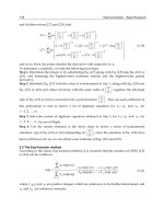
Fig. 3. Isotherm and streamline contours for Gr = 10
6
and Ha = 50: (a) γ = π/6, (b) γ = π/4, (c)
γ = π/3, (d) γ = 5π/12 and (e) γ = π/2 radians

Hydromagnetic Flow with Thermal Radiation

141
Isotherm and streamline plots will be reported for different values of controlling
parameters. The contour lines of isotherm plots correspond to equally-spaced values of the
dimensionless temperature T*, i.e., ΔT* = 0.1, in the range between -0.5 and +0.5. On the
other hand the dimensionless stream function is obtained from the velocity field solution by

integrating the integral
∫
=Ψ
1
0
*dy*u* along constant x* lines, setting Ψ* = 0 at x* = y* = 0.
The contour lines of the streamline plots are correspondent to equally-spaced values of the
dimensionless stream function, unless otherwise specified.
4.1 Influence of the tilting of an enclosure without radiation
A numerical investigation is presented for natural convection of an electrically conducting
fluid in a tilted square cavity in the presence of a vertical magnetic field aligned to the
gravity, i.e., λ = - γ.
In the present study, the Grashof number is fixed as Gr = 10
6
. Computations are carried out
for tilted angles ranging from 0 to π/2 radians, and the thermal radiation is neglected.
Figure 2 shows the isotherm and streamline contours for natural convection in inclined
cavities in the absence of a magnetic field. The multi-cellular inner core consists of a central
roll (designated by “+” in the figures) sandwiched between two rolls. As the tilting angle
decreases, the fluid motion becomes progressively intensive. The temperature is stratified at
the core region in case of γ = π/2 rad. When the tilting angle decreases, this trend is
maintained until γ = π/4 rad. The stratification of the temperature field in the interior begins
to diminish as the inclination angle reaches π/6 rad due to the increasing buoyant action.
The results depicted in Fig. 3 demonstrate the influence of the magnetic field on the fluid
flow and the temperature distributions along with the tilting angle. For relatively strong
Hartmann number (Ha =50), the temperature stratification in the core tends to diminish, and
the thermal boundary layers at the two side walls disappear, together with the decrease in
inclination angle. Also, the streamlines are elongated, and the core region becomes broadly
stagnated. Furthermore, the axes of the streamlines are changed, which is due to the
retarding effect of the Lorentz force. In addition, the flow strength displays maximum at γ =

π/4 rad in this case, then, it decreases when γ reaches π/6 rad. This phenomenon is different
from the previous result for pure free convection; hence, a considerable interaction between
the buoyant and the magnetic forces is evidently caused by the tilting, as the magnitude of
the Lorentz force in the x and y directions is subjected to the inclination angle.
4.2 Effect of the orientation of a magnetic field without radiation
Hydromagnetic flow in a horizontal enclosure (γ = π/2 rad) under a uniform magnetic field
is studied. The changes in the flow and thermal field based on the orientation of an external
magnetic field, which varies from 0 to 2π radians, are investigated in the absence of the
thermal radiation. Assuming constant buoyant action, Gr is fixed as 10
6
.
The source terms caused by the Lorentz force in Eqs. (10) & (11) are such that they are
function of sin
2
λ and cosλsinλ as well as cos
2
λ, which have the common period of π radians.
Thus the numerical simulation is conducted with directional variation of a magnetic field
applied from λ = 0 to π rad on account of the phase difference of π radians.
In Fig. 4, thermo-fluidic behaviour in an enclosure is displayed as to the slanted angle of a
magnetic field when Ha = 50. The flow intensity varies in accordance with the change of λ
and it becomes strongest as λ = 3π/4 rad. This phenomenon can be explained from the flow

Convection and Conduction Heat Transfer

142
retardation induced by direct interaction between the magnetic field and the velocity
component perpendicular to the direction of the magnetic field. As for streamlines, the
orientation of a magnetic field affects the elongation of streamlines. A uni-cellular inner core
is formed along with a transverse magnetic field. Following the change in λ, the inner core

gets a multi-cellular structure accompanying the elongation of streamlines at the central
region. In terms of the thermal field, the tilting of isotherms is most severe with a vertical
magnetic field.



(a) (b) (c) (d)
Fig. 4. Streamlines and isotherms for Gr = 10
6
and Ha = 50: (a) λ = 0, π and 2π; (b) λ = π/4
and 5π/4; (c) λ = π/2 and 3π/2; (d) λ = 3π/4 and 7π/4 radians



(a) (b) (c) (d)
Fig. 5. Streamlines and isotherms for Gr = 10
6
and Ha = 100: (a) λ = 0, π and 2π; (b) λ = π/4
and 5π/4; (c) λ = π/2 and 3π/2; (d) λ = 3π/4 and 7π/4 radians

Hydromagnetic Flow with Thermal Radiation

143
The changes in flow and thermal fields together with λ are illustrated in Fig. 5, in the case of
a strong magnetic field, i.e., Ha = 100. The tendency in the variation of flow and thermal
fields influenced by λ, seems to be similar to that for the prior case. A multi-cellular core
structure, however, start to appear at the later stage comparing with the case of Ha = 50; in
contrast a uni-cellular core structure is recovered at the earlier stage. It is inferred that
stronger magnetic field plays a role to suppress the transition of the inner core structure as λ
varies 0 to π/2 radians. Inclination of isotherms is obvious than Fig. 4. With a vertically

permeated magnetic field, the inclination of isotherms is most conspicuous.
4.3 Effect of combined radiation and a magnetic field
Computation is carried out for free convection of an electrically conducting fluid in a square
enclosure encompassed with radiatively active walls in the presence of a vertically assigned
magnetic field parallel to the gravity. In that case, γ is fixed as π/2 rad so that λ is - π/2 rad.
Radiation-affected temperature and buoyant flow fields in a square enclosure are
demonstrated with Gr = 2 × 10
6
, in the absence of an external magnetic field, i.e., Ha = 0, as
presented in Fig. 6 (a). The radiative interaction between the hot and cold walls is significant
so that the colder region is extended further into the mid-region. The temperature gradients
at the adiabatic walls are steeper owing to the increased interaction by means of the surface
radiation. The flow field displays a multi-cellular structure, and the inner core consists of
two convective rolls in upper and lower halves, respectively.



(a) (b) (c) (d)
Fig. 6. Isotherm and streamline contours with Gr = 2 × 10
6
: (a) Ha = 0, (b) Ha = 10, (c) Ha = 50
and (d) Ha = 100
It is seen that for a weak magnetic field (Ha = 10), as shown in Fig. 6 (b), the isotherms and
streamlines are almost similar to those in the absence of an external magnetic field, i.e.,
Ha = 0. The flow field becomes less intensive a little bit than that corresponding to the
streamline plot in Fig. 6 (a). As a relatively strong magnetic field is applied, i.e., Ha = 50, the
thermal and flow fields are considerably changed as depicted in Fig. 6 (c). The streamlines
are elongated laterally and the axis of the streamline is slanted. The former convective roll at
Ψ* =
T* =

Convection and Conduction Heat Transfer

144
the lower left part of the enclosure moves upward. On the contrary the convective roll
which was at the upper right region moves downward as to increase in the strength of a
magnetic field applied. In the case of the thermal field, severe temperature gradients caused
by the surface radiation are maintained at adiabatic top and bottom walls. In mid-region the
tilting of isotherms coincides with steeper temperature gradient observed by in-between
distance of isotherms getting narrower. These tendencies are preserved until Ha reaches 100,
as illustrated in Fig. 6 (d). Besides such typical influence of a magnetic field as the tilting of
isotherms and streamlines, appears to be emphasised with the suppression of convection in
an enclosure.

Left cold wall Right hot wall
Gr Radiation Ha
C
Nu

R
Nu

C
Nu

R
Nu

T
Nu

0 2.523 0.000 2.523 0.000 2.523
10 2.220 0.000 2.220 0.000 2.220
50 1.118 0.000 1.118 0.000 1.118
Without
100 1.116 0.000 1.116 0.000 1.116
0 4.049 36.733 2.105 38.678 40.783
10 3.754 36.759 1.874 38.641 40.513
50 3.021 36.841 1.368 38.494 39.862
2 × 10
4

With
100 2.997 36.846 1.357 38.487 39.843
0 5.090 0.000 5.090 0.000 5.090
10 4.983 0.000 4.983 0.000 4.983
50 2.997 0.000 2.997 0.000 2.997
Without
100 1.454 0.000 1.454 0.000 1.454
0 6.138 36.486 3.639 38.987 42.624
10 5.986 36.513 3.530 38.970 42.499
50 4.083 36.704 2.068 38.721 40.787
2 × 10
5

With
100 3.174 36.808 1.446 38.537 39.982
0 9.904 0.000 9.904 0.000 9.904
10 9.863 0.000 9.863 0.000 9.863
50 8.891 0.000 8.891 0.000 8.891

Without
100 6.640 0.000 6.640 0.000 6.640
0 10.413 36.047 6.946 39.514 46.460
10 10.339 36.073 6.914 39.499 46.412
50 9.025 36.313 6.050 39.289 45.338
2 × 10
6

With
100 6.699 36.531 4.178 39.054 43.230
Table 1. Nusselt numbers estimated
The rate of heat transfer across the enclosure is attained by evaluating the conductive,
radiative, and total average Nusselt numbers, i.e.,
C
Nu ,
R
Nu , and
T
Nu , respectively, at the
hot and cold walls, and tabulated in Table 1 for various combinations of parameters. From
this table it can be demonstrated that the introduction of a magnetic field suppresses the
convection in the enclosure. With the thermal radiation getting involved in, the radiative
contribution to the combined heat transfer is predominant at both hot and cold walls. In
addition the convective contribution to the combined heat transfer at the cold wall is always
larger than that at the hot wall disregarding the Grashof number and the radiation effect.

Hydromagnetic Flow with Thermal Radiation

145
5. Conclusions

Free convection in a two-dimensional enclosure filled with an electrically conducting fluid
in the presence of an external magnetic field was investigated numerically. The effects of the
controlling parameters on the thermally driven hydromagnetic flows have been scrutinised.
In the first place the changes in the buoyant flow patterns and temperature distributions due
to the tilting of the enclosure were examined neglecting thermal radiation. In general terms,
the effect of the tilting angle on the flow patterns and associated heat transfer was found to
be considerable. The variation of flow strength was affected by the orientation of the cavity
with imposition of the magnetic field because the effective electromagnetic retarding force
in each flow direction was subjected closely to the inclination angle. The flow structure and
the temperature field were enormously affected by the strength of the magnetic field,
regardless of the tilting angle.
Secondly the flow and thermal field variation was investigated in terms of the orientation of
an external magnetic field. The flow intensity and structure varied in accordance with the
change of the direction of an external magnetic field. The flow retardation appeared by
direct interaction between the magnetic field and the velocity component perpendicular to
the direction of the magnetic field. In terms of the thermal field, the tilting of isotherms was
observed.
Finally the effects of combined radiation and a magnetic field on the convective flow and
heat transfer characteristics of an electrically conducting fluid were investigated. It was
concluded that the radiation was the dominant mode of heat transfer and surpassed
convective heat transfer so that it played an important role in developing the hydromagnetic
free convective flow in a differentially heated enclosure.
As a consequence, all the numerical analyses so far have been subjected to the rectangular
enclosure. Hence the future studies are supposed to be related to the general geometries
containing an electrically conducting fluid with the permeation of an external magnetic field
as well as the participation in radiation.
6. Acknowledgment
This work is partly supported by KETEP (Korea Institute of Energy Technology Evaluation
and Planning) under the Ministry of Knowledge Economy, Korea (2008-E-AP-HM-P-19-
0000).

7. References
Bessaih, R.; Kadja, M. & Marty, Ph. (1999). Effect of wall electrical conductivity and magnetic
field orientation on liquid metal flow in a geometry similar to the horizontal
Bridgman configuration for crystal growth.
Int. J. Heat Mass Transfer, Vol.42, pp.
4345-4362
Bian, W.; Vasseur, P., Bilgen, E. & Meng, F. (1996). Effect of an electromagnetic field on
natural convection in an inclined porous layer.
Int. J. Heat and Fluid Flow, Vol.17, pp.
36-44
Chai, J. C.; Lee, H. S. & Patankar, S. V. (1994). Finite-volume method for radiation heat
transfer.
J. Thermophysics and Heat Transfer, Vol.8, pp. 419-425

Convection and Conduction Heat Transfer

146
Chamkha, A. J. (2000). Thermal radiation and buoyancy effects on hydromagnetic flow over
an accelerating permeable surface with heat source or sink.
Int. J. Engng Sci., Vol.38,
pp. 1699-1712
Fusegi, T. & Farouk, B. (1989). Laminar and turbulent natural convection-radiation
interactions in a square enclosure filled with a nongray gas.
Numer. Heat Transfer A,
Vol.15, pp. 303-322
Ghaly, A. Y. (2002). Radiation effects on a certain MHD free-convection flow.
Chaos, Solitons
and Fractals
, Vol.13, pp. 1843-1850
Hua, T. Q. & Walker, J. S. (1995). MHD flow in rectangular ducts with inclined non-uniform

transverse magnetic field.
Fusion Engineering and Design, Vol.27, pp. 703-710
Kolsi, L.; Abidi, A., Borjini, M. N., Daous, N. & Aissia, H. B. (2007). Effect of an external
magnetic field on the 3-D unsteady natural convection in a cubical enclosure.
Numer. Heat Transfer A, Vol.51, pp. 1003-1021
Larson, D. W. & Viskanta, R. (1976). Transient combined laminar free convection and
radiation in a rectangular enclosure.
J. Fluid Mech., Vol.78, pp. 65-85
Mahmud, S. & Fraser, R. A. (2002). Analysis of mixed convection-radiation interaction in a
vertical channel: entropy generation.
Exergy, an Internal Journal, Vol.2, pp. 330-339
Ozoe, H. & Okada, K. (1989). The effect of the direction of the external magnetic field on the
three-dimensional natural convection in a cubical enclosure.
Int. J. Heat Mass
Transfer, Vol.32, pp. 1939-1954
Patankar, S. V. (1980).
Numerical Heat Transfer and Fluid Flow, Hemisphere, McGraw-Hill,
Washington, DC
Raptis, A.; Perdikis, C. & Takhar, H. S. (2004). Effect of thermal radiation on MHD flow.
Applied Mathematics and Computation, Vol.153, pp. 645-649
Rudraiah, N.; Barron, R. M., Venkatachalappa, M. & Subbaraya, C. K. (1995). Effect of a
magnetic field on free convection in a rectangular enclosure.
Int. J. Engng Sci.,
Vol.33, pp. 1075-1084
Seddeek, M. A. (2002). Effects of radiation and variable viscosity on a MHD free convection
flow past a semi-infinite flat plate with an aligned magnetic field in the case of
unsteady flow.
Int. J. Heat Mass Transfer, Vol.45, pp. 931-935
Seki, M.; Kawamura, H. & Sanokawa, K. (1979). Natural convection of mercury in a
magnetic field parallel to the gravity.

J. Heat Transfer, Vol.101, pp. 227-232
Sivasankaran, S. & Ho, C. J. (2008). Effect of temperature dependent properties on MHD
convection of water near its density maximum in a square cavity.
Int. J. Therm. Sci.,
Vol.47, pp. 1184-1194
Thakur, S. & Shyy, W. (1993). Some implementational issues of convection schemes for
finite-volume formulations.
Numer. Heat Transfer B, Vol.24, pp. 31-55
Wang, Q. W.; Zeng, M., Huang, Z. P., Wang, G. & Ozoe, H. (2007). Numerical investigation
of natural convection in an inclined enclosure filled with porous medium under
magnetic field.
Int. J. Heat Mass Transfer, Vol.50, pp. 3684-3689
Part 2
Heat Conduction

7
Transient Heat Conduction in
Capillary Porous Bodies
Nencho Deliiski
University of Forestry
Bulgaria

1. Introduction
Capillarity is a well known phenomenon in physics and engineering. Porous materials such
as soil, sand, rocks, mineral building elements (cement stone or concrete, gypsum stone or
plasterboards, bricks, mortar, etc.), biological products (wood, grains, fruit, etc.) have
microscopic capillaries and pores which cause a mixture of transfer mechanisms to occur
simultaneously when subjected to heating or cooling.
In the most general case each capillary porous material is a peculiar system characterized by
the extremely close contact of three intermixed phases: gas (air), liquid (water) and solid.

Water may appear in them as physically bounded water and capillary water (Chudinov,
1968, Twardowski, Richinski & Traple, 2006). Both the bounded water and the capillary
water can be found in liquid or hard aggregate condition.
Physically bounded water co-operates with the surface of a solid phase of the materials and
has different properties than the free water. The maximum amount of bounded water in
porous materials corresponds to the maximal hygroscopicity, i.e. moisture absorbed by the
material at the 100% relative vapour pressure. The maximum hygroscopicity of the
biological capillary porous bodies is known as fibre saturation point. Capillary water fills
the capillary tube vessels, small pores or sharp, narrow indentions of bigger pores. It is not
bound physically and is called free water. Free water is not in the same thermodynamic
state as liquid water: energy is required to overcome the capillary forces, which arise
between the free water and the solid phase of the materials.
For the optimization of the heating and/or cooling processes in the capillary porous bodies,
it is required that the distribution of the temperature and moisture fields in the bodies and
the consumed energy for their heating at every moment of the process are known. The
intensity of heating or cooling and the consumption of energy depend on the dimensions
and the initial temperature and moisture content of the bodies, on the texture and micro-
structural features of the porous materials, on their anisotropy and on the content and
aggregate condition of the water in them, on the law of change and the values of the
temperature and humidity of the heating or cooling medium, etc. (Deliiski, 2004, 2009).
The correct and effective control of the heating and cooling processes is possible only when
its physics and the weight of the influence of each of the mentioned above as well as of
many other specific factors for the concrete capillary porous body are well understood. The
summary of the influence of a few dozen factors on the heating or cooling processes of the

Convection and Conduction Heat Transfer

150
capillary porous bodies is a difficult task and its solution is possible only with the assistance
of adequate for these processes mathematical models.

There are many publications dedicated to the modelling and computation of distribution of
the temperature and moisture content in the subjected to drying capillary porous bodies at
different initial and boundary conditions. Drying is fundamentally a problem of simulta-
neous heat and mass transfer under transient conditions. Luikov (1968) and later Whitaker
(1977) defined a coupled system of non-linear partial differential equations for heat and
mass transfer in porous bodies. Practically all drying models of capillary porous bodies are
based on these equations and include a description of the specific initial and boundary
conditions, as well as of thermo- and mass physical characteristics of the subjected to drying
bodies (Ben Nasrallah & Perre, 1988, Doe, Oliver & Booker, 1994, Ferguson & Lewis, 1991,
Kulasiri & Woodhead 2005, Murugesan et al., 2001, Zhang, Yang & Liu 1999, etc.).
As a rule the non-defective drying is a very long continuous process, which depending on
the dimensions of the bodies and their initial moisture content can last many hours, days or
even months. However there are a lot of cases in the practice where the capillary porous
bodies are subjected to a relatively short heating and/or cooling, as a result of which a
significant change in their temperature and a relatively small change in their moisture
content occurs. A typical example for this is the change in temperature in building elements
under the influence of the changing surrounding temperature during the day and night or
during fire.
Widely used during the production of veneer, plywood or furniture parts technological
processes of thermal treatment of wood materials (logs, lumber, etc.) with the aim of
plasticizing or ennoblement of the wood are characterized by a controlled change in the
temperature in the volume of the processed bodies, without it being accompanied by
significant changes in their moisture content. In these as well as in other analogous cases of
heating and/or cooling of capillary porous bodies the calculation of the non-stationary
change in the temperature field in the bodies can be carried out with the assistance of
models, which do not take into account the change in moisture content in the bodies. The
number of such published models is very limited, especially in comparison to the existing
large variety of drying models.
Axenenko (1995) presents and uses a 1D model for the computation of the temperature
change in the exposed to fire gypsum plasterboards. According to the author, after

obtaining the temperature fields inside the plasterboard, changes in the material properties
and temperature deformations can be calculated and used as initial data for the study of the
structural behaviour of the entire plasterboard assembly.
Considerate contribution to the calculation of the non-stationary distribution of the
temperature in frozen and non-frozen logs and to the duration of their heating has been
made by H. P. Steinhagen. For this purpose, he, alone, (Steinhagen, 1986, 1991) or with co-
authoring (Steinhagen, Lee & Loehnertz, 1987), (Steinhagen & Lee, 1988) has created and
solved a 1-dimensional, and later a 2-dimensional (Khattabi & Steinhagen, 1992, 1993)
mathematical model, whose application is limited only for u ≥ 0,3 kg.kg
-1
. The development
of these models is dominated by the usage of the method of enthalpy, which is rather more
complicated than its competing temperature method.
The models contain two systems of equations, one of which is used for the calculation of the
change in temperature at the axis of the log, and the other – for the calculation of the
temperature distribution in the remaining points of its volume. The heat energy, which is

Transient Heat Conduction in Capillary Porous Bodies

151
needed for the melting of the ice, which has been formed from the freezing of the
hygroscopically bounded water in the wood, although the specific heat capacity of that ice is
comparable by value to the capacity of the frozen wood itself (Chudinov, 1966), has not been
taken into account. These models assume that the fibre saturation point is identical for all
wood species and that the melting of the ice, formed by the free water in the wood, occurs at
0ºC. However, it is known that there are significant differences between the fibre saturation
point of the separate wood species and that the dependent on this point quantity of ice,
formed from the free water in the wood, thaws at a temperature in the range between -2°C
and -1°C (Chudinov, 1968).
This paper presents the creation and numerical solutions of the 3D, 2D, and 1D

mathematical models for the transient non-linear heat conduction in anisotropic frozen and
non-frozen prismatic and cylindrical capillary porous bodies, where the physics of the
processes of heating and cooling of bodies is taken into account to a maximum degree and
the indicated complications and incompleteness in existing analogous models have been
overcome. The solutions include the non-stationary temperature distribution in the volume
of the bodies for each u ≥ 0 kg.kg
-1
at every moment of their heating and cooling at
prescribed surface temperature, equal to the temperature of the processing medium or
during the time of convective thermal processing.
2. Nomenclature
а = temperature conductivity (m
2
.s
-1
)
b = width (m)
c = specific heat capacity (W.kg
-1
.K
-1
)
d = thickness (m)
D = diameter (m)
L = length (m)
q = internal source of heat, W.m
-3
.s
-1
R = radius (m)

r = radial coordinate: 0
≤
r
≤
R (m)
T = temperature (К)
t = temperature (°C): t = T – 271,15
u = moisture content (kg.kg
-1
= %/100)
x = coordinate on the thickness: 0
≤
x
≤
d/2 (m)
y = coordinate on the width: 0
≤
y
≤
b/2 (m)
z = longitudinal coordinate: 0
≤
z
≤
L/2 (m)
α = heat transfer coefficient between the body and the processing medium
(W.m
-2
.K
-1

)
β = coefficients in the equations for determining of λ
γ = coefficients in the equations for determining of λ
λ = thermal conductivity (W.m
-1
.K
-1
)
ρ = density (kg.m
-3
)
τ = time (s)
φ = angular coordinate (rad)
Δr = distance between mesh points in space coordinates for the cylinders (m)
Δx = distance between mesh points in space coordinates for the prisms (m)
Δτ = interval between time levels (s)

Convection and Conduction Heat Transfer

152
Subscripts:
a = anatomical direction
b = basic (for density, based on dry mass divided to green volume)
bw = bound water
c = center (of the body)
cr = cross sectional to the fibers
d = dimension
e = effective (for specific heat capacity)
fsp = fiber saturation point
fw = free water

i = nodal point in radial direction for the cylinders: 1, 2, 3, …, (R/Δr)+1
or in the direction along the thickness for the prisms: 1, 2, 3, …, [d/(2Δx)]+1
j = nodal point in the direction along the prisms’ width: 1, 2, 3, …, [b/(2Δx)]+1
k = nodal point in longitudinal direction: 1, 2, 3, …, [L/(2Δr)]+1 for the cylinders
or 1, 2, 3, …, [L/(2Δx)]+1 for the prisms
m = medium
nfw = non-frozen water
0 = initial (at 0°C for λ)
p = parallel to the fibers
p/cr = parallel to the cross sectional
p/r = parallel to the radial
r = radial direction (radial to the fibers)
t = tangential direction (tangential to the fibers)
w = wood
x = direction along the thickness
y = direction along the width
z = longitudinal direction
Superscripts:
n = time level 0, 1, 2, …
20 = 20°С
3. Mechanism of heat distribution in capillary porous bodies
During the heating or cooling of the capillary porous materials along with the purely
thermal processes, a mass-exchange occurs between the processing medium and the
materials. The values of the mass diffusion in these materials are usually hundreds of times
smaller than the values of their temperature conductivity. These facts determine a not so big
change in defunding mass in the materials, which lags significantly from the distribution of
heat in them during the heating or cooling. This allows to disregarding the exchange of
mass between the materials and the processing medium and the change in temperature in
them to be viewed as a result of a purely thermo-exchange process, where the heat in them
is distributed only through thermo-conductivity.

Because of this the mechanism of heat distribution in capillary porous bodies can be
described by the equation of heat conduction (also known as the equation of Fourier-
Kirchhoff). Its most compact form is as follows:

Transient Heat Conduction in Capillary Porous Bodies

153

div( grad )
T
cT
q
ρλ
τ
∂
=
−±
∂
. (1)
This form holds for each coordinate system and for each processing medium – both for
immobile and mobile.
In the most general case с, ρ and λ of the capillary porous bodies depend on Т and u, i.e. in
equation (1) the functional dependencies participate с(Т,u), ρ(Т,u) and λ(Т,u).
As it was described in the introduction, the water contained in these bodies can be found in
liquid or hard aggregate condition. It is known that the specific heat capacity of the liquid
(non-frozen) water at 0°С is equal to 4237 J.kg
-1
.K
-1
, and the specific heat capacity of ice is

2261 J.kg
-1
.K
-1
, i.e. almost two times smaller (Chudinov, 1966, 1984). Because of this, the
frozen water in capillary porous bodies causes smaller values of c in comparison to the case,
when the water in them is completely liquid.
The ice in capillary porous bodies can be formed from the freezing of higroscopically
bounded water or of the free water in them. It is widely accepted that the phase transition
of water into ice and vice versa to be expressed with the help of the so-called “latent heat” in
the ice of the frozen body. When solving problems, connected to transient heat conduction
in frozen bodies, it makes sense to include the latent heat in the so-called effective specific
heat capacity c
e
(Chudinov, 1966), which is equal to the sum of the own specific heat
capacity of the body с and the specific heat capacity of the ice, formed in them from the
freezing of the hygroscopically bounded water and of the free water, i.e.

ebwfw
ccc c
=
++. (2)
When solving the problems, it must be taken into consideration that the formation and
thawing of both types of ice in these bodies takes place at different temperature ranges.
Because of this for each of the diapasons in equation (2) the sum of с with
bw
c
and/or
fw
c

(shown below as an example) participates. When modeling processes of transient heat
conduction in anisotropic capillary porous bodies it is also necessary to take into
consideration that the thermal conductivity of these bodies λ apart from Т and u depends
additionally on the direction of the influencing heat flux towards the anatomic directions of
the body – radial, tangential and longitudinal to the fibers.
4. Mathematical models for transient heat conduction in prismatic bodies
If it is assumed, that the anatomical directions of a prismatic capillary porous body coincide
with the coordinate axes, in the absence of an internal source of heat q in equation (1), the
following form of this equation in the Cartesian coordinate system is obtained:

()
(
)
()
(
)
()
()
()
()
e
,,, ,,,
,(,) ,
,,, ,,,
,,
x
yz
Txyz Txyz
cTu Tu Tu

xx
Txyz Txyz
Tu Tu
yyzz
ττ
ρλ
τ
ττ
λλ
⎡
⎤
∂∂
∂
=
+
⎢
⎥
∂∂ ∂
⎣
⎦
⎡
⎤⎡ ⎤
∂∂
∂∂
++
⎢
⎥⎢ ⎥
∂∂∂∂
⎣
⎦⎣ ⎦

. (3)
After the differentiation of the right side of equation (3) on the spatial coordinates x, y, and z,
excluding the arguments in the brackets for shortening of the record, the following
mathematical model of the process of non-stationary heating or cooling (further calling
thermal processing) of the capillary porous bodies with prismatic form is obtained:

Convection and Conduction Heat Transfer

154

2
2
r
er
2
2
2
22
p
t
tp
22
TT T
c
Tx
x
TT T T
Ty T z
yz
λ

ρλ
τ
λ
λ
λλ
∂∂∂∂
⎛⎞
=+ +
⎜⎟
∂∂∂
∂
⎝⎠
∂
⎛⎞
∂
∂∂∂ ∂
⎛⎞
++ + +
⎜⎟
⎜⎟
∂∂ ∂∂
∂∂
⎝⎠
⎝⎠
(4)
with an initial condition

(
)
0

,,,0Tx
y
zT
=
(5)
and boundary conditions:
•
during the time of thermal processing of the prisms at their prescribed surface
temperature, equal to the temperature of the processing medium:

(
)
(
)
(
)
(
)
m
0,,, ,0,, ,,0,Tyz Txz Txy T
τ
τττ
===, (6)
•
during the time of convective thermal processing of the prisms:

[]
r
m
r

(0,,,) (0,,,)
(0,,,) ()
(0, , , )
Tyz yz
Tyz T
xyz
τα τ
τ
τ
λτ
∂
=− −
∂
, (7)

[]
t
m
t
(,0,,)
(,0,,)
(,0,,) ()
(,0,,)
xz
Tx z
Tx z T
yxz
ατ
τ
τ

τ
λτ
∂
=− −
∂
, (8)

[]
p
m
p
(,,0,)
(,,0,)
(,,0,) ()
(,,0,)
xy
Txy
Txy T
zxy
ατ
τ
τ
τ
λτ
∂
=− −
∂
. (9)
The system of equations (4) ÷ (9) presents a 3D mathematical model, which describes the
change in temperature in the volume of capillary porous bodies with prismatic form during

the time of their thermal processing at corresponding initial and boundary conditions.
When the length of the subjected to thermal processing body exceeds its thickness by at least
()
p
rt
2
22,5
λ
λ
λ
÷
+
times, then the heat transfer through the frontal sides of the body can be
neglected, because it does not influence the change in temperature in the cross-section,
which is equally distant from the frontal sides. In these cases for the calculation of the
change in T in this section (i.e. only along the coordinates x and y) the following 2D model
can be used:

2
2
22
t
r
er t
22
TT T T T
c
Tx T
y
xy

λ
λ
ρλ λ
τ
⎛⎞
∂
∂∂∂∂ ∂ ∂
⎛⎞
=+ ++
⎜⎟
⎜⎟
∂∂∂ ∂∂
∂∂
⎝⎠
⎝⎠
(10)
with an initial condition

(
)
0
,,0Tx
y
T
=
(11)
and boundary conditions:

Transient Heat Conduction in Capillary Porous Bodies

155
• for thermal processing of the prisms at their prescribed surface temperature:

(
)
(
)
(
)
m
0, , ,0,Ty Tx T
τ
ττ
==, (12)
•
for convective thermal processing of the prisms:

[]
r
m
r
(0, , ) (0, , )
(0, , ) ( )
(0, , )
Ty y
Ty T
xy
τα τ
τ
τ

λτ
∂
=− −
∂
, (13)

[]
t
m
t
(,0,)
(,0,)
(,0,) ()
(,0,)
x
Tx
Tx T
yx
ατ
τ
τ
τ
λτ
∂
=− −
∂
. (14)
When the thickness of the body is smaller than its width by at least 2 ÷ 3 times, and than its
length by at least
()

p
r
22,5
λ
λ
÷ times, then the non-stationary change in T, for example along
the radial direction x of the body, coinciding with its thickness in the section, equally distant
from the frontal sides, can be calculated using the following 1D model:

2
2
r
er
2
TT T
c
Tx
x
λ
ρλ
τ
∂∂∂∂
⎛⎞
=+
⎜⎟
∂∂∂
∂
⎝⎠
(15)
with an initial condition

(
)
0
,0Tx T
=
(16)
and boundary conditions:
•
for thermal processing of the prisms at their prescribed surface temperature:

(
)
(
)
m
0,TT
τ
τ
= , (17)
•
for convective thermal processing of the prisms:

[]
r
m
r
(0, ) (0, )
(0, ) ( )
(0, )

T
TT
x
τατ
τ
τ
λτ
∂
=− −
∂
. (18)
5. Mathematical models for transient heat conduction in cylindrical bodies
The mechanism of the heat distribution in the volume of cylindrical capillary porous bodies
during their thermal processing can be described by the following non-linear differential
equation with partial derivatives, which is obtained from the equation (3) after passing in it
from rectangular to cylindrical coordinates (Deliiski, 1979)

()()
(
)
()
(
)
(
)
(
)
() () ()
()
()

()
()
22
er
222
22 2
2
p
r
p
22
,, ,, ,, ,,
11
,, ,
,
,,, ,, ,, ,,
1
,
Trz Trz Trz Trz
cTu Tu Tu
rr
rr
Tu
Tu Trz Trz Trz Trz
Tu
Tr Tz
rz
ττττ
ρλ
τ

φ
λ
λτ τ τ τ
λ
φ
⎡⎤
∂∂∂∂
=+++
⎢⎥
∂∂
∂∂
⎢⎥
⎣⎦
⎧⎫
∂
∂⎡∂⎤⎡∂⎤ ∂ ⎡∂⎤
⎪⎪
++++
⎨⎬
⎢⎥⎢⎥ ⎢⎥
∂∂ ∂ ∂∂
∂
⎣⎦⎣⎦ ⎣⎦
⎪⎪
⎩⎭
. (19)

Convection and Conduction Heat Transfer

156

If heating or cooling cylindrical bodies of material, which is homogenous in their cross
section, the distribution of T in their volume does not depend on φ, but only depends on r
and z. Consequently, when excluding the participants in the equation (19), containing φ and
when also omitting the arguments in the brackets for the shortening of the record, the
following 2D mathematical model is obtained, which describes the change of temperature in
the volume of capillary porous bodies with cylindrical form:


2
2
r
er
2
2
2
p
p
2
1TTT T
c
rr T r
r
TT
Tz
z
λ
ρλ
τ
λ
λ

⎛⎞
∂∂∂∂∂
⎛⎞
=
++ +
⎜⎟
⎜⎟
⎜⎟
∂∂∂∂
∂
⎝⎠
⎝⎠
∂
∂∂
⎛⎞
++
⎜⎟
∂∂
∂
⎝⎠
(20)

with an initial condition

(
)
0
,,0Trz T
=
(21)

and boundary conditions:
•
for thermal processing of the bodies at their prescribed surface temperature:


(
)
(
)
(
)
m
0, , ,0,Tz Tr T
τ
ττ
==, (22)

• for convective thermal processing of the bodies:


[]
r
m
r
(0,,) (0,,)
(0,,) ()
(0,,)
Tz z
Tz T

rz
τα τ
τ
τ
λτ
∂
=− −
∂
, (23)

[]
p
m
p
(,0,)
(,0,)
(,0,) ()
(,0,)
r
Tr
Tr T
zr
ατ
τ
τ
τ
λτ
∂
=− −
∂

. (24)

When the length of the body exceeds its diameter by at least
()
p
r
22,5
λ
λ
÷ times, then the
heat transfer through the frontal sides of the body can be neglected, because it does not
influence the change in temperature of its cross section, which is equally distant from the
frontal sides. In such cases, for the calculation of the change in T only along the coordinate r
of this section, the following 1D model can be used:

2
2
r
er
2
1TTT T
c
rr T r
r
λ
ρλ
τ
⎛⎞
∂∂∂∂∂
⎛⎞

=++
⎜⎟
⎜⎟
⎜⎟
∂∂∂∂
∂
⎝⎠
⎝⎠
(25)
with an initial condition

(
)
0
,0Tr T
=
(26)
and with boundary conditions, which are identical to the ones in equations (17) and (18), but
with derivative of T along r instead of along x in (18).

Transient Heat Conduction in Capillary Porous Bodies

157
6. Transformation of the models for transient heat conduction in suitable
form for programming
Analytical solution of mathematical models, which contain non-linear differential equations
with partial derivatives in the form of (4) and (20), is practically impossible without
significant simplifications of these equations and of their boundary conditions.
For the numerical solution of models with such equations the methods of finite differences
or of the finite elements can be used. When the bodies have a correct shape – prismatic or

cylindrical, the method of finite differences is preferred, because its implementation requires
less computational resources from the computers.
For the numerical solution of the above presented models for transient heat conduction it
makes sense to use the explicit form of the finite-difference method, which allows for the
exclusion of any simplifications. The large calculation resources of the contemporary
computers eliminate the inconvenience, which creates the limitation for the value of the step
along the time coordinate
τ
Δ
by using the explicit form (refer to equation (47)).
According to the main idea of the finite-difference method, the temperature, which is a
uninterrupted function of space and time, is presented using a grid vector, and the
derivatives
T
x
∂
∂
,
T
y
∂
∂
,
T
z
∂
∂
and
T
τ

∂
∂
are approximated using the built computational mesh
along the spatial and time coordinates through their finite-difference (discrete) analogues.
For this purpose the subjected to thermal processing body, or 1/8 of it in the presence of
mirror symmetry towards the other 7/8, is “pierced” by a system of mutually perpendicular
lines, which are parallel to the three spatial coordinate axes. The distances between the lines,
also called as the step of differentiation, is constant for each coordinate direction (Fig. 1). The
knots from 0 to 6 with temperatures accordingly from
0
T to
6
T are centers for the presented
and neighboring it volume elements. The length of the sides of the volume element xΔ ,
yΔ

and zΔ are steps of differentiation, the size of which determines the distance between the
separate knots of the mesh. The entire time of thermal processing of the body is also
separated into definite number n intervals (steps) with equal duration
τ
Δ
. A volume
element of a subjected to thermal processing body used for the solution of equation (4) is
shown on Fig. 1, together with its belonging part from the rectangular calculation mesh.


Fig. 1. A volume element of the body with a built on it calculation mesh for the solution of
equation (4) using the explicit form of the finite-difference method

Convection and Conduction Heat Transfer

158
As a result of the described procedures, the process for the solution of the non-linear
differential equation with partial derivatives (4) is transformed to the solution of the
equivalent to it system of linear finite-difference equations, requiring the carrying out of
numerous one-type, but not complicated algebraic operations. In the built in the body 3D
rectangular mesh, the heat transfer is taken into consideration only along its gradient lines.
For each cross point of three mesh lines, called a knot, a finite-difference equation is derived,
using which the temperature of this knot is calculated.
Finite-difference equations are obtained by substituting derivatives in the differential
equation (4), with their approximate expressions, which are differences between the values
of the function in selected knots of the calculation mesh. The temperature in knot 0 with
coordinates (
i
x ,
j
y
,
k
z ,
n
τ
) on Fig. 1 is designated as
n
kji
TT
,,0
= , and the temperature in
neighboring knots accordingly as
11,,

n
i
j
k
TT
+
= (knot 1),
21,,
n
i
j
k
TT
−
= (knot 2),
3,1,
n
i
j
k
TT
+
=
(knot 3),
4,1,
n
i
j
k
TT

−
= (knot 4),
5,,1
n
ijk
TT
+
= (knot 5), and
6,,1
n
ijk
TT
−
= (knot 6). For the
calculation of temperature
0
T in each following moment of time (1)n
τ
+
Δ the values of the
temperatures from
1
T
to
6
T
in the preceding moment n
τ
Δ
need to be known.

6.1 Discrete analogues of models for transient heat conduction in prismatic bodies
The transformation of the non-linear differential equation with partial derivatives (4) in its
discrete analogue with the help of the explicit form of the finite-difference method is carried
out using the shown on Fig. 2 coordinate system for the positioning of the knots of the
calculation mesh, in which the distribution of the temperature in a subjected to thermal
processing capillary porous body with prismatic form is computed.


Fig. 2. Positioning of the knots in the calculation mesh on 1/8 of the volume of a subjected to
thermal processing prismatic capillary porous body
For the carrying out of the differentiation of λ along Т in equation (4), it is necessary to have
the function
()
T
λ
in the separate anatomical directions of the capillary porous body. For
the purpose of determination of subsequent transformations of the models, we accept that

Transient Heat Conduction in Capillary Porous Bodies

159
the functions
()
r
T
λ
,
(
)
t

T
λ
and
(
)
p
T
λ
are linear both for containing ice, as well as for not
containing ice bodies and are described with an equation of the kind:

[
]
0
1 ( 273,15)T
λλγ β
=+− . (27)
Then after carrying out the differentiation of λ along Т in equation (4) and substituting in it
with finite differences of the first derivative along the time and the first and second
derivatives along the spatial coordinates, the following system of equations is obtained:
()
1 2
,, ,, 1,, 1,, ,, ,, 1,,
e0r,,
22
2
, 1, , 1, ,, ,, , 1.
0t , ,
22
2( )

1273,15
2( )
1 ( 273,15)
nn n n n nn
ijk ijk i jk i jk ijk ijk i jk
n
ijk
nn n nn
ij k ij k ijk ijk ij k
n
ijk
TT T T T TT
cT
xx
TT T TT
T
yy
ρλγβ β
τ
λγ β β
+
+− −
+− −
⎧
⎫
−+−−
⎪
⎪
⎡⎤
=

+− + +
⎨
⎬
⎣⎦
Δ
ΔΔ
⎪
⎪
⎩⎭
⎧
+− −
⎡⎤
++− +
⎣⎦
ΔΔ
2
,, 1 ,, 1 ,, ,, ,, 1
0p , ,
22
2( )
1( 273,15)
nn n nn
ijk ijk ijk ijk ijk
n
ijk
TT T TT
T
zz
λγ β β
+− −

⎫
⎪
⎪
+
⎨
⎬
⎪
⎪
⎩⎭
⎧
⎫
+− −
⎪
⎪
⎡⎤
++− +
⎨
⎬
⎣⎦
ΔΔ
⎪
⎪
⎩⎭
(28)
After transformation of the equation (28) it is obtained, that the value of the temperature in
whichever knot of the built in the volume of a subjected to thermal processing body 3D
mesh at the moment
(1)n
τ
+

Δ is determined depending on the already computed values
for the temperature in the preceding moment n
τ
Δ
using the following system of finite
differences equations:
()( )()
()( )()
1
,, ,,
2
0r
,, 1,, 1,, ,, ,, 1,,
2
2
0t
,, , 1, , 1, ,, ,, , 1,
2
e
0p
2
1 273,15 2
1 273,15 2
1
nn
ijk ijk
nnnnnn
ijk i jk i jk ijk ijk i jk
nnnnnn
ijk ij k ij k ijk ijk ij k

TT
TTTTTT
x
TTTTTT
c
y
z
λ
ββ
λ
γτ
ββ
ρ
λ
β
+
+− −
+− −
=+
⎡⎤
⎡⎤
+− +−+− +
⎢⎥
⎣⎦
⎣⎦
Δ
Δ
⎡⎤
⎡⎤
++ + − + − + − +

⎢⎥
⎣⎦
⎣⎦
Δ
++
Δ
()( )()
2
,, ,, 1 ,, 1 ,, ,, ,, 1
273,15 2
nnnnnn
ijk ijk ijk ijk ijk ijk
TTTTTT
β
+− −
⎧ ⎫
⎪ ⎪
⎪ ⎪
⎪ ⎪
⎪ ⎪
⎨ ⎬
⎪ ⎪
⎪ ⎪
⎡⎤
⎡⎤
⎪ ⎪
−+−+−
⎢⎥
⎣⎦
⎪ ⎪

⎣⎦
⎩ ⎭
. (29)
The initial condition (5) in the 3D mathematical model is presented using the following
finite differences equation:

0
0
,,
TT
kji
= . (30)
The boundary conditions (6) ÷ (9) get the following easy for programming form:
•
for thermal processing of the prisms at their prescribed surface temperature:

1
m
1
1,,
1
,1,
1
,,1
+
+
+
+
===
nn

ji
n
ki
n
kj
TTTT
, (31)
•
for convective thermal processing of the prisms:

1
2, , 1, , m
1
1, ,
1, ,
1
nn
jk jk
n
jk
jk
TGT
T
G
+
+
+
=
+
where

()
r
1, ,
0r 1, ,
[1 273,15 ]
jk
n
jk
x
G
T
α
λγ β
Δ
=
+−
, (32)

Convection and Conduction Heat Transfer

160

()
1
,2, ,1, m
1
t
,1, ,1,
,1,
0t ,1,

where
1
[1 273,15 ]
nn
ik ik
n
ik ik
n
ik
ik
TGT
x
TG
G
T
α
λγ β
+
+
+
Δ
==
+
+−
, (33)

()
1
,,2 ,,1 m
p

1
,,1 ,,1
,,1
0p , ,1
where
1
[1 273,15 ]
nn
ij ij
n
ij ij
n
ij
ij
TGT
x
TG
G
T
α
λγ β
+
+
+
Δ
==
+
+−
. (34)
In the boundary conditions (31) ÷ (34) is reflected the requirement for the used for the

solution of the models computation environment of FORTRAN, that the knots of the mesh,
which are positioned on the corresponding surface of the subjected to thermal processing
prism, to be designated with number 1, i.e. 1 ≤ i ≤ M; 1 ≤ j ≤ N; 1 ≤ k ≤ KD (Dorn &
McCracken 1972). Using the system of equations (29) ÷ (34) the distribution of the tempera-
ture in subjected to thermal processing prismatic materials can be calculated, whose radial,
tangential and parallel to the fibers direction coincide with its coordinate axes х, у and z.
Since the subjected to thermal processing in the practice prismatic materials usually do not
have a clear radial or clear tangential sides, but are with partially radial or partially
tangential, then in equation (29) instead of the coefficients λ
0
in the observed two anatomical
directions their average arithmetic value can be substituted, which determines the thermal
conductivity at 0°С cross sectional to the body’s fibers λ
0cr
:

0r 0t
0cr
2
λ
λ
λ
+
=
. (35)
Also the thermal conductivity at 0°С in the direction parallel to the fibers
λ
0p
can be
expressed through

λ
0cr
using the equation

0p p/cr 0cr
K
λ
λ
=
, (36)
where the coefficient
0p
p/cr
0cr
K
λ
λ
=
depends on the type of the capillary porous material.
For the unification of the calculations it makes sense to use one such step of the calculation
mesh along the spatial coordinates ∆
x = ∆y = ∆z (refer to Fig. 2). Taking into consideration
this condition, and also of equations (35) and (36), the system of equations (29) becomes
1
,, ,,
,,
0cr
1, , 1, , , 1, , 1, p/cr , , 1 , , 1 p/cr , ,
2
e

22
, , 1, , , , , 1, p/cr , ,
1 ( 273,15)
()(42)
()()(
nn
ijk ijk
n
ijk
nnnn nn n
i jk i jk ij k ij k ijk ijk ijk
nn nn
ijk i jk ijk ij k ijk
TT
T
TTTTKTT KT
cx
TT TT KT
β
λγΔτ
ρΔ
β
+
+− +− +−
−−
=+
⎡⎤
+−
⎣⎦
⎡⎤

+ ++++ + −+ +
⎣⎦
+− +− +
2
,, 1
)
nn
ijk
T
−
⎧ ⎫
⎪ ⎪
⎪ ⎪
⎨ ⎬
⎪ ⎪
⎡⎤
⎪ ⎪
−
⎣⎦
⎩ ⎭
. (37)
In this case in equations (32) and (33) instead of
r
α
and
t
α
,
cr
α

must be used, and instead of
0r
λ
and
0t
λ
,
0cr
λ
must be used.
The discrete analogue of the 2D model, in which equations (10) ÷ (14) participate, becomes

(
)
(
)
()()
,1,1,,1,1,
1
0cr
,,
22
2
e
,1, ,,1
1 273,15 4
nnnnnn
ij i j i j ij ij ij
nn
ij ij

nn nn
ij i j ij ij
TTTTTT
TT
cx
TT TT
β
λγτ
ρ
β
+− +−
+
−−
⎧
⎫
⎡⎤
+
−+++−+
⎣⎦
⎪
⎪
Δ
=+
⎨
⎬
⎡⎤
Δ
⎪
⎪
+− +−

⎢⎥
⎣⎦
⎩⎭
(38)

Transient Heat Conduction in Capillary Porous Bodies

161
with an initial condition

0
0
,
TT
ji
=
(39)
and boundary conditions:
•
for thermal processing of the prisms at their prescribed surface temperature:

1
m
1
1,
1
,1
+
+
+

==
nn
i
n
j
TTT
, (40)
•
for convective thermal processing of the prisms:

()
1
2, 1, m
1
cr
1, 1,
1,
0cr 1,
where
1
[1 273,15 ]
nn
jj
n
jj
n
j
j
TGT
x

TG
G
T
α
λγ β
+
+
+
Δ
==
+
+−
, (41)

()
1
,2 ,1 m
1
cr
,1 ,1
,1
0cr ,1
where
1
[1 273,15 ]
nn
ii
n
ii
n

i
i
TGT
x
TG
G
T
α
λγ β
+
+
+
Δ
==
+
+−
. (42)
The discrete analogue of the 1D model, in which equations (15) ÷ (18) participate, becomes

(
)
(
)
(
)
{
}
2
1
0cr

11 1
2
e
1 273,15 2
nn n nn n nn
ii i ii i ii
TT T TT T TT
cx
λ
γτ
ββ
ρ
+
+− −
Δ
⎡⎤
=+ +− +−+−
⎣⎦
Δ
(43)
with an initial condition

0
0
TT
i
=
(44)
and boundary conditions:
•

for thermal processing of the prisms at their prescribed surface temperature:

1
m
1
1
++
=
nn
TT , (45)
•
for convective thermal processing of the prisms:

()
1
1
cr
21m
11
1
0cr 1
 where
1
[1 273,15 ]
nn
n
n
x
TGT
TG

G
T
α
λγ β
+
+
Δ
+
==
+
+−
. (46)
Using the system of equations (37) and (30) ÷ (36) of the 3D case, (38) ÷ (42) of the 2D case
and (43) ÷ (46) of the 1D case, the integration of the differential equation (4) and of its
reduced along the spatial coordinates analogues, is transformed to a consequent
determination of the values of T in the knots of the calculation mesh, built in the subjected to
thermal processing prismatic material, where during the computations the distribution of T
is used in the preceding moment, distanced from the current by
τ
Δ
.
The value of the step
τ
Δ
is determined by the requirement for stability of the solution of the
corresponding system of equations. It must not exceed the smaller of the two values
obtained from the equations

(
)

()
(
)
()
2
2
emax max
emin min
dmin dmax
,( ,)
,( ,)
and
,,
cT u T ux
cT u T ux
KT u KT u
ρ
ρ
ττ
λλ
Δ
Δ
Δ= Δ=
, (47)

Convection and Conduction Heat Transfer

162
in which
min

T and
max
T are correspondingly the smallest and biggest of all values of the
temperatures, encountered in the initial and boundary conditions of the heat transfer when
solving the mathematical model, and
d
K
is a coefficient, reflecting the dimensioning of the
heat flux when calculating the step
τ
Δ
: for a 3D heat flux
dp/cr
6KK
=
; for a 2D heat flux
d
4K = and for a 1D heat flux
d
2K
=
.
6.2 Discrete analogues of models for transient heat conduction in cylindrical bodies
For the obtaining of a discrete analogues of equations (20) ÷ (24) the explicit form of the
finite-difference method has been used in a way comparable to the reviewed above case of
2D thermal processing of prismatic bodies. The transformation of the non-linear differential
equation with partial derivatives (20) in its discrete analogue is carried out using the shown
on Fig. 3 coordinate system for the positioning of the knots from the calculation mesh, in
which the distribution of temperature in the longitudinal section of subjected to thermal
processing cylindrical body is calculated. The calculation mesh for the solution of the 2D

model with the help of the finite-differences method is built on ¼ of the longitudinal section
of the cylindrical body due to the circumstance that this ¼ is mirror symmetrical towards
the remaining ¾ of the same section.


Fig. 3. Positioning of the knots of the calculation mesh on ¼ of the longitudinal section of a
subjected to thermal processing cylindrical body
Taking into consideration equations (2) and (27) and using the coefficient
0p
p/r
0r
K
λ
λ
=
, after
applying the explicit form of the finite-differences method to equations (20) ÷ (24), they are
transformed into the following system of equations:

()
()
()
()
()()
,
1, 1, p/r , 1 , 1
1
0r
,,
2

e
p/r , 1, ,
22
1, , p/r , 1 ,
1 273,15
1
22
1
n
ik
nn nn
i k i k ik ik
nn
ik ik
nnn
ik i k ik
nn nn
i k ik ik ik
T
TTKTT
TT
cr
KT T T
i
TT KTT
β
λγτ
ρ
β
−+ −+

+
−
−−
⎧
⎫
⎡⎤
+−
⎪
⎪
⎣⎦
⎪
⎪
⎪
⎪
⎡
⎤
++ + −
⎪
⎪
Δ
⎢
⎥
=
++
⎨
⎬
⎢
⎥
Δ
++ −

⎪
⎪
⎢
⎥
−
⎣
⎦
⎪
⎪
⎪
⎪
⎡
⎤
−+ −
⎪
⎪
⎢
⎥
⎣
⎦
⎩⎭
(48)

Transient Heat Conduction in Capillary Porous Bodies

163
with an initial condition

0
,0ik

TT
=
(49)
and boundary conditions:
•
for heating or cooling of the bodies at their prescribed surface temperature:

1
m
1
1,
1
,1
+++
==
nn
i
n
k
TTT , (50)
•
for convective heating or cooling of the bodies in the processing medium:

()
1
2, 1, m
1
r
1, 1,
1,

0r 1,
where
1
[1 273,15 ]
nn
kk
n
kk
n
k
k
TGT
x
TG
G
T
α
λγ β
+
+
+
Δ
==
+
+−
, (51)

()
1
p

,2 ,1 m
1
,1 ,1
,1
0p ,1
where
1
[1 273,15 ]
nn
ii
n
ii
n
i
i
x
TGT
TG
G
T
α
λγ β
+
+
Δ
+
==
+
+−
. (52)

The discrete analogue of the 1D model, in which equations (25), (26), (17) and (18)
participate, takes the form

(
)
()()
1
0r
2
2
e
11 1 1
1 273,15
1
2
1
n
i
nn
ii
nn n nn nn
ii i ii ii
T
TT
cr
TT T TT TT
i
β
λγτ
ρ

β
+
−+ − −
⎧
⎫
⎡⎤
+−
⎣⎦
⎪
⎪
Δ
⎪
⎪
=+
⎨
⎬
⎡⎤
Δ
⎪
⎪
+−+ − + −
⎢⎥
−
⎪
⎪
⎣⎦
⎩⎭
(53)
with an initial condition presented through equation (44) and boundary conditions,
presented through equations (45) and (46), where in (46) instead of

cr
α
and
0cr
λ
,
r
α
and
0r
λ
are used. The value of the
τ
Δ
, which guarantees the obtaining of robust solutions for
the presented models, is determined by the condition for stability, described by equation
(47). When solving the 2D model
dp/r
4KK
=
, and when solving the 1D model
d
2K = in
(47).
7. Mathematical description of the thermo-physical characteristics of the
capillary porous bodies
The mathematical description of the thermo-physical characteristics of the capillary porous
bodies consists of the deduction of summarized dependencies as a function of the factors
which have an influence on them, which with maximum precision correspond to the their
experimentally determined values in the interesting for the practice sufficiently wide ranges

for the change in the factors. It is necessary to have such a description when solving the
above presented mathematical models of the transient heat conduction in capillary porous
bodies.
The following thermo-physical characteristics are present in these models: specific heat
capacity, thermal conductivity and density of the capillary porous bodies.
The mathematical description of the above mentioned characteristics of the wood, which is a
typical representative of the studied bodies, is shown as an example below.