Hydrodynamics Natural Water Bodies Part 2 pot
Bạn đang xem bản rút gọn của tài liệu. Xem và tải ngay bản đầy đủ của tài liệu tại đây (4.36 MB, 25 trang )
Hydrodynamics – Natural Water Bodies
12
data and the other is the calculation based on estimation of transport parameters such as
travel time and dispersion coefficients. Since exact morphological data are often unavailable,
the parameter estimation technique is more promising.
In both approaches, tracer experiments are needed to provide field data for water quality
models calibration and validation procedures. Indeed, model calibration is often a weak step
in its development and using experimental tracer techniques, the calibration and validation
problems can be solved satisfactorily, improving the needed feasibility of the early warning
systems used by many water supply utilities.
Tracer experiments are typically conducted with artificial fluorescent dyes (like rhodamine
WT) (Fig. 11), whose concentrations are easily measured with a fluorometre. These tracers
should be easily detected, non toxic and non-reactive, as well as, have high diffusivity, low
acidity and sorption for a quasi-conservative behaviour.
Fig. 11. Rhodamine spreading after their injection in a river Mondego reach
Based on field experiments data, many investigators have derived semi-empirical equations
(Hubbard et al., 1982; Chapra, 1997; Addler et al., 1999) or applied one-dimensional models
(Duarte & Boaventura, 2008) to calculate experimental longitudinal dispersion coefficients
from concentration time curves at consecutive sampling sites, using the analytical solution
of first order decay kinetics (Table 1).
The injected tracer dye mass must be calculated considering the water volume estimated in
the river reach or reservoir system and the fluorometre detection limit. Specific problems of
the application of tracers to surface water researches include the photosensitivity of dyes,
such as fluorescence tracers, and recovery efficiency, which may imply the use of correction
techniques for tracer losses. The tracer mass recovered at each site allowed the assessment of
the importance of physical and biochemical river processes by quantifying precipitation,
sorption, retention and assimilation losses. Usually, total tracer mass losses resulting from
all these sinks can reach 40 to 50% of the injected mass (Duarte & Boaventura, 2008; Addler
et al., 1999).
In some recent experiments, a gas tracer (SF
6
) has been shown to be a powerful tool for
examining mixing, dispersion, and residence time on large scales in rivers and estuaries
A Hydroinformatic Tool for Sustainable Estuarine Management
13
(Caplow et al. 2004) as an alternative method to dye tracer experiments used for advection
and dispersion characterisation.
AVERAGE
VELOCITY (ms
-1
)
TRAVEL TIME
(h)
D
ISPERSION
COEFFICIENT (m
2
s
-1
)
RECOVERED
MASS
MONITORING
PROGRAM
REACH
EXPER. DUFLOW EXPER. DUF LOW EXPER. DUFLOW (%)
S1 – S2 0.526 Var. 2:37 2:35 14 10 57
3 rd. S2 – S3 0.497 Var. 2:41 2:41 51 45 56
(Nov 90) S3 – S5 0.473 Var. 3:21 3:19 37 35 55
S1 – S3 0.511 Var. 5:18 5:16 34 - -
S1 – S5 0.497 Var. 8:38 8:35 35 - -
1 st. S1 – S2 1.105 Var. 1:14 1:14 52 40 62
(Dec 89) S2 – S3 0.949 Var. 1:24 1:24 61 70 62
S1 – S3 1.023 Var. 2:38 2:38 58 - -
Table 1. Hydraulic and dispersion parameters estimation using tracer dye experiments in a
non-tidal reach of river Mondego
The dispersion processes in rivers are combined with a specific dynamic characterized by a
decrease in maximum dye concentration (Fig. 12). The distribution of the tracer in all
directions follows the sluggish injection into the channel. In non-tidal rivers, the lateral and
vertical dispersion processes are almost always faster than the continuing longitudinal
dispersion process.
DECEMBER-89 SAMPLING PROGRAM
(Flow=140 m
3
/s - flood situation)
0,00
0,10
0,20
0,30
0,40
0,50
0,60
8:00
8:15
8:30
8:45
9:00
9:15
9:30
9:45
10:00
10:15
10:30
10:45
11:00
11:15
11:30
11:45
12:00
12:15
Time (h)
Concentration ( g/L)
Model Results Site 1 Site 2 Site 3
R=0,98
R=0,93
R=0,97
Fig. 12. River Mondego model calibration: correlation between field tracer experiment data
and model results.
One-dimensional modelling is a reasonably reliable tool to be considered for estimating the
distribution of solutes in large rivers. Complex processes, for example in dead zones or
downstream from the confluence of two rivers, have to be investigated by direct
measurements and should be described by two-dimensional transport models. Calculation
of net advection in tidal rivers is fairly straightforward, but longitudinal dispersion is
difficult to determine a priori, and the application of two or three-dimensional transport
models are often required.
Hydrodynamics – Natural Water Bodies
14
Ever increasing computational capacities provide the development of powerful and user-
friendly mathematical models for the simulation and forecast of quality changes in receiving
waters after land runoff, mining and wastewater discharges.
The results of several research works have showed that the linkage of tracer experimental
approach with mathematical modelling can constitute a power and useful operational tool
to establish better warning systems and to improve management practices for the efficiently
protection of water supply sources and, consequently, public health.
2.4 Mathematical modelling
Numerical modelling is a multifaceted tool that enables a better understanding of physical,
chemical and biological processes in the water bodies, based on a “simplified version of the
real” described by a set of equations, which are usually solved by numerical methods.
The models to be used for the implementation of the WFD management strategies should
ideally have the highest possible degree of integration to comply with the integrated river
basin approach, coupling hydrological, hydrodynamic, water quality and ecological
modules as a function of the specific environmental issues to analyse.
The Mondego Estuary (MONDEST) model was conceptualized (Fig. 13) as an integrated
hydroinformatic tool, linking hydrodynamics, water quality and residence time (TempResid)
modules (Duarte, 2005).
Bathymetry
Mesh
generation
Boundary
SCENARIO SCENARIO SCENARIO
RESULTS RESULTS
HYDRODYNAMIC
MODULE
TRANSPORT
MODULE
TempResid
MODULE
Tidal prism and flows
Currents velocity
Nutrients balance
Dispersive characteristics
Salinity distribution
Saltwater intrusion
• spatial distribution
Residence time:
• discharge type effect
Wetlands
Bathymetry
Mesh
generation
Boundary
Bathymetry
Mesh
generation
Boundary
SCENARIO SCENARIO SCENARIO
RESULTS RESULTS
HYDRODYNAMIC
MODULE
TRANSPORT
MODULE
TempResid
MODULE
Tidal prism and flows
Currents velocity
Nutrients balance
Dispersive characteristics
Salinity distribution
Saltwater intrusion
• spatial distribution
Residence time:
• discharge type effect
Wetlands
Fig. 13. The MONDEST model conceptualization
The formulation of an accurate model requires the best possible definition of the geometry
and bathymetry of the water body and the interactions with the boundary conditions, as
stated in previous items.
This model is based on generalized computer programmes RMA2 and RMA4 (WES-HL,
1996; 2000), which were applied and adapted to this specific estuarine ecosystem. The
CEWES version of RMA4 is a revised version of RMA4 as developed by King & Rachiele
(1989).
The RMA2 programme solves depth-integrated equations of fluid mass and momentum
conservation in two horizontal directions by the finite element method (FEM) using the
Galerkin Method of weighted residuals. The shape (or basis) functions are quadratic for
velocity and linear for depth. Integration in space is performed by Gaussian integration.
Derivatives in time are replaced by a nonlinear finite difference approximation.
A Hydroinformatic Tool for Sustainable Estuarine Management
15
The RMA4 programme solves depth-integrated equations of the transport and mixing
process using the Galerkin Method of weighted residuals. The form of the depth averaged
transport equation is given by equation (1)
()
0
xy
ccc c c Rc
huv D D kc
txyxxyy h
(1)
Where
h =water depth;
c = concentration of pollutant for a given constituent;
t = time;
u, v = velocity in x direction and y direction;
Dx, Dy, = turbulent mixing (dispersion) coefficient;
k = first order decay of pollutant;
σ = source/sink of constituent;
R(c) = rainfall/evaporation rate.
As with the hydrodynamic model RMA2, the transport model RMA4 handles one-
dimensional segments or two-dimensional quadrilaterals, triangles or curved element
edges. Spatial integration of the equations is performed by Gaussian techniques and the
temporal variations are handled by nonlinear finite differences consistent with the method
described for RMA2.
The numerical computation was carried out for all Mondego estuary spatial domains.
Several sections were carefully selected and used for calibrating and analysis of the
simulation results (Duarte, 2005). The legend includes the designation, section code and
their distance to the mouth of the estuary (Fig. 14).
136000
140000
144000
148000
152000
156000
160000
348000
352000
356000
N0
N
2
N
1
N3
N4
N5
N6
S5
S4
S3
S2
S
1
CODE SECTION NAME DISTANCE (km)
N0 Estuary mouth 0.0
N1 Recreational harbor 1.3
N2 Figueira Bridge 2.8
N3 Gramatal 6.3
N4
Cinco Irmãos
7.4
N5 Maria da Mata sluices 10.0
N6 Fo
j
aPum
p
in
g
Station 15.7
N7 River Arunca mouth 20.9
N8 Formoselha Brid
g
e 28.6
N9 Pereira Bridge 31.4
S1 Gala Brid
g
e
(
Lota
)
2.6
S2 Armazéns creek (Negra) 4.4
S3 R ive
r
Pranto mouth 5.4
S4
A
reeiro novo
6.7
S5
A
lvo sluices 8.7
Fig. 14. The MONDEST model finite elements mesh and outline of the control sections
Hydrodynamics – Natural Water Bodies
16
The size of the elements to consider in the spatial discrimination of the simulated domain of
numerical models must be established as a function of larger or smaller spatial gradients
than those displayed by the variables (water level and velocity) in that domain. In the case
of the Mondego estuary, since the south arm was the preferred object for studying, the
network of finite elements was refined in that sub-domain, thereby reducing the maximum
area of its (triangular) elements to 500 m
2
(Duarte, 2005).
In the MONDEST model, the hydrodynamic module provides flow velocities and water
levels for the water quality module, whose results acts as input on the TempResid module,
feeding the constituents concentration over the aquatic system. The post-processing and
mapping of model results was performed using SMS package (Boss SMS, 1996).
The TempResid module was integrally developed in this research work aiming to compute
RT values of each water constituent (conservative or not) and allowing to map its spatial
distribution over all the estuarine system, considering different simulated management
scenarios.
RT value of a substance was calculated for each location and instant, as an interval of time
that is necessary for that corresponding initial mass to reduce to a pre-defined percentage of
that value. In this work, a value of 10% was adopted for the residual concentration of the
substance, attending to the fact that the effect of the re-entry of the mass in the estuary
during tidal flooding is considered (a significant effect for dry-weather river flow rates).
The determination of the RT in several stations along the estuary, where the eutrophication
gradient occurred, was carried out by applying the TempResid programme to the results of
the simulations that were performed with the transport module of the MONDEST model.
Figure 15 shows an example of the MONDEST model transport module results for the
management scenario considered as the most favourable to macroalgae blooms occurrence
(Duarte, 2005), due to low freshwater inputs and consequent reduction of estuarine waters
renovation (scenario RT1).
0
10
20
30
40
50
60
70
80
90
100
0 24 48 72 96 120 144 168 192 216 240
Concentration (%)
Time (hour)
Scenario RT1
estuary mouth Gala bridge river Pranto mouth
RT criteria (10% )
Fig. 15. Residence time computation using TempResid module
A Hydroinformatic Tool for Sustainable Estuarine Management
17
This graph presents the concentration decrease of a conservative constituent, in three control
points (N0 - estuary mouth; S1 - Gala bridge/Lota; and S3- Pranto river mouth), due to
estuarine flushing currents, considering the well known re-entrance phenomena at the
estuary mouth.
2.5 Simulated management scenarios
For hydrodynamic modelling purpose, a wide range (sixteen) of management scenarios
were judiciously selected covering a representative set of hydraulic conditions (Table 2),
resulting from the combination of typical tidal amplitudes (0.60, 1.15, and 1.60 m) and
freshwater flow inputs (from Mondego and Pranto).
Freshwater flow (m
3
.s
-1
)
TIDE
Mondego Pranto Medium Spring Neap
15
0 H 1 H 2 H3
15 H 4 - -
30 H 5 - -
75 0 H 6 H 7 H 8
340
0 H 9 H 10 H 11
15 H 12 - -
30 H 13 - -
500 30 - H 14 -
800 30 - H 15 H 16
Table 2. Simulated management scenarios for the hydrodynamic modelling
For the Mondest transport model calibration and validation, the salinity was adopted as a
natural tracer. Several management scenarios (nine) were also carefully selected (Table 3)
considering the most representative hydrodynamic conditions in order to estimate salt
wedge propagation into the estuary and to identify the areas (in both arms) where
favourable salinity values for macroalgae growth can potentiate the estuarine
eutrophication vulnerability.
Freshwater flow (m
3
.s
-1
)
TIDE
Mondego Pranto Medium Spring Neap
15
0 SL 1 SL 6 SL 9
15 SL 2 - -
30 SL 3 - -
75 0 SL 4 SL 7 -
340 15 SL 5 SL 8 -
Table 3. Simulated management scenarios for the hydrodynamic modelling
For the RT values calculation using the TempResid module, the simulated management
scenarios (fourteen) were defined considering not only the most critical hydrodynamic
conditions, but also by carefully selecting distinct pollutant load characteristics (e,g. location,
duration and type of the discharge event, instant of tidal cycle when the release occurs) and
Hydrodynamics – Natural Water Bodies
18
constituent decay rates (Table 4) in order to assess and confirm the highest eutrophication
vulnerability of the inner areas of the Mondego estuary south arm, due to the expected
occurrence of higher RT values.
SCENARIO
RIVER FLOW
(m
3
.s
-1
)
TIDE LOAD
DECAY RATE
(day
-1
)
Mondego Pranto
RT 1
15
0
medium
point
0
RT 2 spring
RT 3 neap
RT 4
medium
1
RT 5 10
RT 6 15
0
RT 7 1
0
RT 8 75
RT 9 340
RT 10
15
diffuse
RT 11 1
RT12
75
0
RT 13 1
RT 14 0,5
Table 4. Simulated management scenarios for estuarine residence time calculation
In this work only a few examples of the very large amount of MONDEST model results
obtained for those different simulated scenarios can be presented. The main aim of the
following item will be to highlight the evident influence of hydrodynamics (tidal regime
and freshwater inflows) on estuarine residence time spatial variation, which can play a
special role in estuarine eutrophication vulnerability assessment.
3. Results and discussion
3.1 Hydrodynamic modelling
Hydrodynamic modelling results allowed to evaluate the water level and magnitude of
currents velocity in both arms during tidal ebbing and flooding situations, and to assess the
influence of tidal and freshwater inflows regimes on its variability.
For dry weather conditions, the higher velocity values were obtained in the southern arm,
near Gala Bridge, reaching 0.35 (neap tide, scenario H3) to 0.70 m.s
-1
(spring tide, scenario
H2) while in the northern arm these maximum values (which occur in the section N4) are
lower, reaching 0.33 (neap tide) to 0.60 m.s
-1
(spring tide), at 1km upstream the Figueira da
Foz bridge. These results are depicted on Figure 16 mapping the effect of extreme tidal
regimes on maximum currents velocity magnitude during the flooding period and
considering dry-weather conditions.
In the southern arm, the flooding time, which decreases at the inner zones, is much shorter
than the ebbing time, due to shallow waters and to large intertidal mudflats areas. This
A Hydroinformatic Tool for Sustainable Estuarine Management
19
asymmetry is influenced by the tidal regime and has a fast increase into the inner areas of
this arm reaching 2.5 hours: 5 hours for flooding and 7.5 hours for ebbing time. In the
northern arm, between the sections N1 and N4, there is a little delay of fifteen minutes in the
high tide occurrence and a bigger delay in ebb tide (about two hours).
Fig. 16. Effect of tidal regime on ebbing maximum values of currents velocity magnitude
(scenarios H2 and H3)
Figure 17(a) shows an example of the tidal regime effect in the mean velocity magnitude
(MVM) variation, at section N4 (where maximum values of this parameter occurred). It
should be noted that for a neap tide, the VMM during the tidal flooding period is almost an
half of the value reached for a typical sprig tide.
For upstream estuarine sections, water surface levels in high tide are similar, but, in ebb
tide, water surface level increases in the inner section due to the effect of the estuarine
bathimetry (elevation of bottom level) (Fig. 17b).
Fig. 17. (a) Effect of tidal regime on ebbing maximum values of currents velocity magnitude
(section N4); (b) Surface water level variation along the estuarine system (N1, N7, N8)
3.2 Model calibration and validation
The velocities and water levels field data obtained from the sampling programme were used
for model calibration and validation. Figure 18 shows an example of a specific procedure
performed in section S1 (Gala bridge/Lota) for the parameter “surface water level (SWL)”.
Two different sensitivity analyses were carried out to define the accurate values to adopt for
the main calibration parameters used in both (hydrodynamic and water transport) modules
of Mondest model: one for the Manning bottom friction coefficient (n) and horizontal Eddy
Hydrodynamics – Natural Water Bodies
20
viscosity coefficient (E
h
); and the other for the horizontal dispersion coefficient (D
h
). For
each calibration parameter, three different values were tested comparing field data with the
corresponding model results.
Fig. 18. Hydrodynamic module calibration (spring tide) and validation (neap tide)
(station S1)
For the simulated management scenarios and based on calculated correlation coefficients,
the best agreements were obtained considering the following parameters values: the
ordered pair (n=0.02 m
-1/3
.s; E
h
= 20 m
2
.s
-1
), for the hydrodynamic module; and D
h
= 30 m
2
.s
-1
,
for the water transport module.
A more detailed description of these sensitivity analyses (scenarios, results and discussion)
can be found in Duarte (2005).
3.3 Tidal prism and flow estimation
In this work a new approach was developed for tidal flow estimation, based on the previous
tidal prism calculation using mathematical modelling. The adopted approach allows to
consider the temporal variation of the cross section area during the tidal cycle and, mainly,
the real asymmetry of tidal flooding and ebbing periods verified in the inner estuarine areas.
Tidal prisms were calculated as the difference between the water volume in a specific high tide
and the correspondent previous ebb tide, which can be automatically given by the query tools
of the post-processor module (SMS). Figure 19 shows the spatial variation of tidal
Fig. 19. Tidal prism spatial variation in both estuary arms (flooding of scenario H1)
A Hydroinformatic Tool for Sustainable Estuarine Management
21
prism for the both estuary arms (north and south) based on this procedure calculation for
each control sections along the Mondego estuary, considering the flooding period of the
scenario H1.
The mean tidal flow estimation in each estuarine section can be performed using the
correspondents’ tidal prism values and the real duration of the ebbing and flood events. The
mean tidal flow values obtained for several hydrodynamic scenarios in the sections N0 and
S1 are summarized in Table 5.
flooding ebbing flooding ebbing flooding ebbing
H 1
9.178 9.894 6.25 6.25 408 440
H 2 12.02 13.063 6.25 6.25 534 581
H 3 5.818 5.692 6.25 6.25 259 253
H 7 14.792 15.386 6,25 6,25 657 684
H 10
11.387 12.089 6.00 6.50 527 517
H 1 2.334 2.341 5.50 7.00 118 93
H 2 3.265 3.276 5.50 7.00 165 130
H 3 1.269 1.266 6.00 6.50 59 54
H 7 3.449 345 5.50 7.00 174 137
H 10
3.325 3.337 5.50 7.00 168 132
S1
Section Scenario
Tidal prism (hm
3
) Duration (h) Mean tidal flow (m
3
.s
-1
)
N0
Table 5. Synthesis of mean tidal flow calculation (sections N0 and S1)
3.4 Hydrodynamic influence on estuarine salinity distribution
The analysis of the salinity distribution in the estuary had, as a primary goal, the
identification of the areas that, throughout the tidal cycle, present salinity values within the
range of 17 to 22‰, defined by Martins et al. (2001) as the most favourable for algal growth
in this specific aquatic ecosystem.
The Pranto river inflow in estuary southern arm has shown a strong influence on salinity
distribution decreasing drastically its values to a range far from the one defined as the most
favourable for this estuarine eutrophication process. Figure 20 shows the opening Alvo
sluices effect on southern arm salinity gradients caused by Pranto river flow discharge of
30 m
3
.s
-1
, during the ending of ebbing and the beginning of tidal flooding periods (scenarios
SL 3 and SL1) (Duarte & Vieira, 2009a).
Fig. 20. Effect of Pranto river flow discharge on estuarine salinity distribution (high tide)
SLUICES OPEN SLUICES CLOSED
Hydrodynamics – Natural Water Bodies
22
The effect of tidal regime on saline wedge propagation into the Mondego estuary can be
assessed by comparing the saline front position at high or ebb tide achieved for the extreme
tidal amplitudes (spring and neap tides). For the simulated conditions (scenarios SL2 and
SL3) a difference of about 4 km in the estuarine saline wedge intrusion was observed:
12.5 km for a spring tide and only 8.5 km for a neap tide. Figure 21 depicts the differences on
the saline wedge return (ebb tide) for these two extreme tidal regimes.
Fig. 21. Effect of tidal regime on saline wedge reflux (ebb tide) (scenarios SL2 and SL3)
3.5 Hydrodynamic influence on estuarine residence time distribution
During the warm season (late spring and summer), the Alvo sluices are almost closed
(scenario RT1). For this operational condition, the RT values near Pranto mouth station can
quintuplicate when compared with those resulting from a Pranto river flow discharge of
15 m
3
.s
-1
(scenario RT6), both under dry-weather conditions (low river Mondego inflows).
Figure 22 shows this sensitive increase on flushing capacity of the Mondego estuary south
arm due to Pranto river discharges from Alvo sluices opening.
Fig. 22. Effect of Pranto river discharge on RT values distribution (scenarios RT1 and RT6)
For the other hand, when the Alvo sluices remain closed the salinity and the RT values
inside the southern arm are strongly influenced by tidal regime. Figure 23 illustrates the
gradient of RT spatial distribution, which was mapped applying the TemResid module
computing availability for the simulation of management scenarios RT2 and RT3.
Simulation results for these two tidal scenarios showed a RT values increase of 50% for a
neap tide, when compared with a spring tide, both in the south arm and in the north arm
reach, between N1 and N2 control points. This increase is smoothed in the northern arm
inner areas, with the lowest increase (only 17%) at the Mondego estuary mouth. The
A Hydroinformatic Tool for Sustainable Estuarine Management
23
minimum RT values (3.2 days) occurred in the Mondego estuary mouth (N0) and in the
mesotrophic wetland zone of the south arm (near station S2). The maximum RT values (9.5
days) were obtained for the zone (near station S3) with higher eutrophication vulnerability.
Concerning the periodicity of tidal regime recurrence, its effect could be very relevant for
estuarine biochemical processes with a time scale lower than 6 days.
Fig. 23. Effect of tidal regime on RT values distribution (scenarios RT2 and RT3)
4. Conclusion
The analysis of the results obtained in the performed simulations allows the confirmation
that there is a significant influence of bathymetry in the spatial variation of the RT along the
Mondego estuary and consequently, the definition of typical (unique) values for each one of
its arms becomes inadequate if they are not associated to local and specific hydrodynamic
scenarios.
The results obtained from hydrodynamic modelling have shown a strong asymmetry of
ebbing and flooding times in the inner estuary south arm areas due to their complex geo-
morphology (extensive wetlands and salt marsh zones, over 75% of its total area). This
information allows a better understand of the estuarine circulation pattern, since tide is the
major driving force of the southern arm flushing capacity, when the Alvo sluices remain
closed. Indeed, the absence of the Pranto river discharge (a typical dry-weather condition)
drastically increases salinity and RT values in the inner estuary southern arm and,
consequently, the nutrients availability for algae uptake is higher, enhancing estuarine
vulnerability to eutrophication.
From the analysis of the results obtained, it is possible to conclude that in both arms of this
estuary, the tidal prism volumes are influenced by the bathymetry (extensive wetland
areas), tidal regime and freshwater inputs. However, the influence of the tidal regime on the
tide prism values is much greater than that of the freshwater inflows, and it is possible to
verify that those values do not increase proportionally to the incremental values of the
Mondego River flow rate.
The knowledge of the ebbing and flooding duration asymmetry is crucial for a more
accurate tidal flow calculation, based on previous tidal prim estimation using mathematical
modelling tools. With this new approach for mean tidal flow estimation the variation of
cross section area can also be computed increasing the feasibility of the obtained results.
For the simulated conditions a difference of about 4 km in the estuarine saline wedge
intrusion was observed: 12.5 km for a spring tide and only 8.5 km for a neap tide. However,
a sensitive surface water elevation was monitored in the upper control section (N8), near the
Hydrodynamics – Natural Water Bodies
24
Formoselha bridge (located 30 km upstream the estuary mouth), during a spring tide
propagation.
For medium typical tide, drought conditions and conservative constituents, simulation
results showed that estuarine RT values range between 6 days (at both arms) and 4 days in
the downstream reach of its two arms confluence (control point N1).
The development of integrated methodologies linking tracer experimental approach with
hydroinformatic tools (based on 2D and 3D mathematical models) is of paramount interest
because they can constitute a accurate and useful operational tool to establish better
warning systems and to improve management practices for efficiently protecting water
sources and, consequently, public health.
The MONDEST model developed and applied in this work allowed the evaluation and
ranking of potential mitigation measures (like nutrient loads reduction or dredging works
for hydrodynamic circulation improvement). So, the proposed methodology, integrating
hydrodynamics and water quality, constitutes a powerful hydroinformatic tool for
enhancing estuarine eutrophication vulnerability assessment, in order to contribute for
better water quality management practices and to achieve a true sustainable development.
5. References
Addler, M.J.; Stancalie, G. & Raducu, C. (1999). Integrating tracer with remote sensing
techniques for determining dispersion coefficients of the Dâmbovita River,
Romania. In: Integrated Methods in Catchment Hydrology—Tracer, Remote Sensing and
New Hydrometric Techniques (Proceedings of IUGG 99-Symposium HS4), IAHS Publ.
No. 258, pp. 75-81, Birmingham, July, 1999.
Bendoricchio, G.D.B. (2006). A water-quality model for the lagoon of Venice, Italy. Ecological
Modelling, 184, pp. 69–81, ISSN 0304-3800
Boss SMS (1996). Boss Surface Modeling System-User’s Manual, Brigham Young University
Press, USA.
Burwell, D.C. (2001). Modelling the spatial structure of estuarine residence time : eulerian and
lagrangian approaches. PhD. Thesis, College of Marine Science, University of South
Florida, USA.
Caplow, T.; Schlosser, P.; Ho, D. T. & Enriquez, R. C. (2004). Effect of tides on solute flushing
from a strait: imaging flow and transport in the East River with SF
6
. Environ. Sci.
Technol., Vol.38, No.17, pp. 4562–4571, ISSN 1520-5851
Chapra, S. C. (1997). Surface Water Quality Modelling, McGraw-Hill, New York, USA.
Cucco, A., Umgiesser, G.; Ferrarinb, C.; Perilli A., Canuc, D.M. & Solidoroc, C. (2009).
Eulerian and lagrangian transport time scales of a tidal active coastal basin,
Ecological Modelling, Vol.220, No.7, pp. 913–922, ISSN 0304-3800
Cucco, A. & Umgiesser, G. (2006). Modelling the Venice lagoon water residence time.
Ecological Modelling, Vol.193, pp. 34–51, ISSN 0304-3800
Cunha, P.P. & Dinis, J. (2002). Sedimentary dynamics of the Mondego estuary. In: Aquatic
ecology of the Mondego river basin. Global importance of local experience, Pardal M.A.,
Marques J.C. & Graça M.S. (eds.), pp. 43-62, Coimbra University Press, IBSN 972-
8704-04-6, Coimbra, Portugal.
Dronkers, J. & Zimmerman, J.T.F. (1982). Some principles of mixing in tidal lagoons. In:
Oceanologica Acta. Procedings of the International Symposium on Coastal Lagoons, pp.
107–117, Bordeaux, France, September 9–14, 1981
A Hydroinformatic Tool for Sustainable Estuarine Management
25
Dettmann E. (2001). Effect of water residence time on annual export and denitrification of
nutrient in estuaries: a model analysis. Estuaries, Vol.24, No.4, pp. 481–490, ISSN
1559-2723
Duarte, A.A.L.S. & Vieira, J.M.P. (2009a). Mitigation of estuarine eutrophication proceses by
controlling freshwater inflows. In: River Basin Management V, ISBN 978-1-84564-198-
6, and WIT Transactions on Ecology and the Environment, pp. 339-350, ISSN: 1743-
3541, WIT Press, Ashusrt, Reino Unido.
Duarte, A.A.L.S. & Vieira, J.M.P. (2009b). Estuarine hydrodynamic as a key-parameter to
control eutrophication processes. WSEAS Transactions on Fluid Mechanics, Vol.4,
No.4, (October 2009), pp. 137-147, ISSN 1790-5087
Duarte, A.A.L.S. & Boaventura, R.A.R (2008). Pollutant dispersion modelling for Portuguese
river water uses protection linked to tracer dye experimental data. WSEAS
Transactions on Environment and Development, Vol.4, No.12, (December 2008), pp.
1047-1056, ISSN 1790-5079
Duarte, A.A.L.S. (2005). Hydrodynamics influence on estuarine eutrophication processes. PhD.
Thesis, Civil Engineering Dept., University of Minho, Braga, Portugal (in
Portuguese).
Duarte, A.A.L.S.; Pinho, J.L.S.; Vieira, J.M.P. & Seabra-Santos, F. (2002). Hydrodynamic
modelling for Mondego estuary water quality management. In: Aquatic ecology of
the Mondego river basin. Global importance of local experience, Pardal M.A., Marques
J.C. & Graça M.S. (eds.), pp. 29-42, Coimbra University Press, IBSN 972-8704-04-6,
Coimbra, Portugal.
Duarte, A.A.L.S.; Pinho, J.L.S.; Pardal, M.A.; Neto, J.M.; Vieira, J.M.P. & Seabra-Santos, F.
(2001). Effect of Residence Times on River Mondego Estuary Eutrophication
Vulnerability. Water Science and Technology, Vol.44, No.2/3, pp. 329-336, ISSN 0273-
1223.
Harremoës, P. & Madsen, H. (1999). Fiction and reality in the modelling world – Balance
between simplicity and complexity, calibration and identifiably, verification and
falsification. Water Science and Technology, Vol.39, No.9, pp. 47–54, ISSN 0273-1223.
Hubbard, E.F.; Kilpatrick, F.A.; Martens, C.A. & Wilson, J.F. (1982). Measurement of Time of
Travel and Dispersion in Streams by Dye Tracing, Geological Survey, U.S. Dept. of the
Interior, Washington, EUA
JPL (1996). A Collection of Global Ocean Tide Models. Jet Propulsion Laboratory, Physical
Oceanography Distributed Active Archive Center, Pasadena, CA.
King, I.P. & Rachiele, R.R. (1989). Program Documentation: RMA4 - A two Dimensional Finite
Element Water Quality Model, Version 3.0, ed. Resource Management Associates,
January, 1989.
Luketina, D. (1998). Simple tidal prism model revisited. Estuarine Coastal and Shelf Science,
Vol.46, pp.77–84, ISSN 0272-7714
Marinov, D. & Norro, A.J.M.Z. (2006). Application of COHERENS model for hydrodynamic
investigation of Sacca di Goro coastal lagoon (Italian Adriatic Sea shore). Ecological
Modelling, Vol.193, No.1, pp. 52–68, ISSN 0304-3800
Monsen, N.E.; Cloern, J.E. & Lucas, L.V. (2002). A comment on the use of flushing time,
residence time, and age as transport time scales. Limnology & Oceanography, Vol.47,
No.5, (May 2002), pp. 1545–1553, ISSN 0024-3590
Hydrodynamics – Natural Water Bodies
26
Oliveira, A. P. & Baptista, A.M. (1997). Diagnostic modelling of residence times in estuaries.
Water Resources Reseach, Vol.33, pp.1935–1946, ISSN 0024-3590
Paerl, H.W (2006). Assessing and managing nutrient-enhanced eutrophication in estuarine
and coastal waters: interactive effects of human and climatic perturbations.
Ecological Engineering, Vol.26, No.1, (January 2006), pp. 40-54, ISSN 0925-8574
Pardal, M.A.; Cardoso, P.G.; Sousa, J.P.; Marques, J.C. & Raffaelli, D.G. (2004). Assessing
environmental quality: a novel approach. Marine Ecology Progress Series, Vol.267,
pp. 1-8, ISSN 0171-8630.
Sanford, L.; Boicourt, W. & Rives, S. (1992). Model for estimating tidal flushing of small
embayments. Journal of Waterway, Port, Coastal and Ocean Engineering, Vol.118, No.6,
pp. 913–935, ISSN 1943-5460
Stamou, A.I.; Nanou-Giannarou, K. & Spanoudaki, K. (2007). Best modelling practices in the
application of the Directive 2000/60 in Greece. Proceedings of the 3rd IASME/WSEAS
Int. Conference on Energy, Environment, Ecosystems and Sustainable Development, pp.
388-397, Agios Nikolaos, Crete Island, Greece, July 24-26, 2007.
Takeoka, H. (1984). Fundamental concepts of exchange and transport time scales in a coastal
sea. Continental Shelf Research, Vol.3, No.3, pp. 311–326, ISSN 0278-4343
Thomann, R.V. & Linker, L.C. (1998). Contemporary issues in watershed and water quality
modelling for eutrophication control. Water Science & Technology, Vol.37, pp. 93-102,
ISSN 0273-1223
Valiela, I., McClelland, J., Hauxwell, J., Behr, P.J., Hersh, D. & Foreman, K. (1997)
Macroalgae blooms in shallow estuaries: controls, ecophysiological and ecosystem
consequences. Limnology & Oceanography, Vol.42, No.5, (January 1997), pp. 1105–
1118, ISSN 0024-3590
Vieira, J.M.P; Duarte, A.A.L.S.; Pinho, J.L.S. & Boaventura, R.A. (1999). A Contribution to
Drinking Water Sources Protection Strategies in a Portuguese River Basin,
Proceedings of the XXII World Water Congress, CD-Rom, Buenos Aires, Argentina,
September, 5-7, 1999.
Wang, C.F.; Hsu,M. & Kuo, A.Y.(2004). Residence time of the Danshuei Estuary, Taiwan.
Estuarine, Coastal and Shelf. Science, Vol.60, pp. 381-393, ISSN 1906-0015
WES-HL (1996). Users Guide to RMA2 Version 4.3. US Army Corps of Engineers, Waterways
Experiment Station Hydraulics Laboratory, Vicksburg, USA.
WES-HL (2000). Users Guide to RMA4 WES Version 4.5. US Army Corps of Engineers,
Waterways Experiment Station Hydraulics Laboratory, Vicksburg, USA.
2
Hydrodynamic Control of Plankton
Spatial and Temporal Heterogeneity
in Subtropical Shallow Lakes
Luciana de Souza Cardoso
1
, Carlos Ruberto Fragoso Jr.
3
,
Rafael Siqueira Souza
2
and David da Motta Marques
2
Universidade Federal do Rio Grande do Sul (UFRGS)
1
Instituto de Biociências
2
Instituto de Pesquisas Hidráulicas (IPH)
3
Universidade Federal de Alagoas (UFAL)
Centro de Tecnologia
Brazil
1. Introduction
During the last 200 years, many lakes have suffered from eutrophication, implying an
increase of both nutrient loading and organic matter (Wetzel, 1996). An aspect that has
often been neglected in freshwater systems is the fact that phytoplankton is often not evenly
distributed horizontally in space in shallow lakes. Although the occurrence of
phytoplankton patchiness in marine systems has been known for a long time (e.g., Platt et
al., 1970; Steele, 1978; Steele & Henderson, 1992), phytoplankton in shallow lakes is often
assumed to be homogeneously distributed. However, there are various mechanisms that
may cause horizontal heterogeneity in shallow lakes. For example, grazing by aggregated
zooplankton and other organisms may cause spatial heterogeneity in phytoplankton
(Scheffer & De Boer, 1995). Submerged macrophyte beds may be another mechanism,
through reduction of resuspension by wave action and allopathic effects on the algal
community (Van den Berg et al., 1998). For large shallow lakes, wind can be a dominant
factor leading to both spatial and temporal heterogeneity of phytoplankton (Carrick et al.,
1993), either indirectly by affecting the local nutrient concentrations due to resuspended
particles, or directly by resuspending algae from the sediment (Scheffer, 1998). In the
management of large lakes, prediction of the phytoplankton distribution can assist the
manager to decide on an optimal course of action, such as biomanipulation and regulation
of the use of the lake for recreation activities or potable water supply (Reynolds, 1999).
However, it is difficult to measure the spatial distribution of phytoplankton. Mathematical
modeling of a phytoplankton can be an important alternative methodology in improving
our knowledge regarding the physical, chemical and biological processes related to
phytoplankton ecology (Scheffer, 1998; Edwards & Brindley, 1999; Mukhopadhyay &
Bhattacharyya, 2006).
Over the past decade there has been a concerted effort to increase the realism of ecosystem
models that describe plankton production as a biological indicator of eutrophication. Most
Hydrodynamics – Natural Water Bodies
28
of this effort has been expended on the description of phytoplankton in temperate lakes;
thus, multi-nutrient, photo-acclimation models are now not uncommon (e.g., Olsen &
Willen, 1980; Edmondson & Lehman, 1981; Sas, 1989; Fasham et al., 2006; Mitra & Flynn,
2007; Mitra et al., 2007). In subtropical lakes, eutrophication has been intensively studied,
but only with a focus on measuring changes in nutrient concentrations (e.g., Matveev &
Matveeva, 2005; Kamenir et al., 2007). A wide variety of phytoplankton models have been
developed. The simplest models are based on a steady state or on the assumption of
complete mixing (Schindler, 1975; Smith, 1980; Thoman & Segna, 1980). Phytoplankton
models based on more complex vertical 1-D hydrodynamic processes give a more realistic
representation of the stratification and mixing processes in deep lakes (Imberger &
Patterson, 1990; Hamilton et al., 1995a; Hamilton et al., 1995b). However, the vertical 1-D
assumption might be too restrictive, especially in large shallow lakes that are poorly
stratified and often characterized by significant differences between the pelagic and littoral
zones. In these cases, a horizontal 2-D model with a complete description of the
hydrodynamic and ecological processes can offer more insight into the factors determining
local water quality.
Currently, computational power no longer limits the development of 2-D and 3-D models,
and these models are being used more frequently. Of the wide diversity of 2-D and 3-D
hydrodynamic models, most were designed to study deep-ocean circulation or coastal,
estuarine and lagoon zones (Blumberg & Mellor, 1987; Casulli, 1990). However, only a few
models are coupled with biological components (Rajar & Cetina, 1997; Bonnet & Wessen,
2001).
In this chapter, we present the results of comparative modeling of two subtropical shallow
lakes where the wind, and derived hydrodynamics, and river flow act as the main factors
controlling plankton dynamics on temporal and spatial scales. The basic hypothesis is that
wind and wind derived-hydrodynamics are the main factor determining the spatial and
temporal distribution of plankton communities (Cardoso et al. 2003; Cardoso & Motta
Marques, 2003, 2004a, 2004b, 2004c, 2009), in association with point incoming river flows.
The spatial heterogeneity of phytoplankton in Lake Mangueira is influenced by
hydrodynamic patterns, and identifying zones with a higher potential for eutrophication
and phytoplankton patchiness (Fragoso Jr. et al., 2008). The spatial patterns of chlorophyll-a
concentrations generated by the model were validated both with a field data set and with a
cloud-free satellite image provided by a Terra Moderate Resolution Imaging
Spectroradiometer (MODIS) with a spatial resolution of 1.0 km.
1.1 Study areas
Itapeva Lake is the first (N→S) in a system of interconnected fresh-water coastal lakes on the
northern coast of the state of Rio Grande do Sul, Brazil (Fig. 1). The lake has an elongated
shape (30.8 km × 7.6 km) and a surface area of ≈125 km
2
, and is shallow, with a maximum
depth of 2.5 m. The lake is oriented according to the prevailing wind direction (NE – SW
quadrants), where the northern part is more constricted and consequently the water is more
confined. Two rivers enter the lake: Cardoso River, in the northern part, and Três Forquilhas
River in the southern part. The former is small and the flow was not important for the input;
however, the contribution of the latter river was modeled and influenced the spatial pattern.
Lake Mangueira (33°1'48"S 52°49'25"W) is a large freshwater ecosystem in southern Brazil
(Fig. 2), covering a total area of 820 km
2
, with a mean depth of 2.6 m and maximum depth of
Hydrodynamic Control of Plankton Spatial and
Temporal Heterogeneity in Subtropical Shallow Lakes
29
Lake
Q
uadros
Lake Ita
p
eva
Três Forquilhas
Basin
Atlantic Ocean
North
Station
Center
Station
South
Station
Fig. 1. Itapeva Lake in southern Brazil, with the three sampling points (North, Center and
South).
Patos Lagoon
Lake Mangueira
Mirim Lake
ESEC Taim
Atlantic Ocean
Rio Grande
Santa Vitória do Palmar
Porto Alegre
N
Taim Wetland
Lake Mangueira
Taim
Wetland
TAMAN
TAMAC
TAMAS
Fig. 2. Lake Mangueira in southern Brazil. The meteorological and sampling stations in the
North, Center and South parts of Lake Mangueira are termed TAMAN, TAMAC and
TAMAS, respectively.
6.5 m. Its trophic state ranges from oligotrophic to mesotrophic (annual mean PO
4
concentration 35 mg m
-3
, varying from 5 to 51 mg m
-3
). This lake is surrounded by a variety
of habitats including dunes, pinus forests, grasslands, and two wetlands. This
heterogeneous landscape harbors an exceptional biological diversity, which motivated the
Brazilian federal authorities to protect part of the entire hydrological system as the Taim
Ecological Station in 1991 (Garcia et al., 2006). The watershed (ca. 415 km
2
) is primarily used
Hydrodynamics – Natural Water Bodies
30
for rice production, and many of the local waterbodies are used for irrigation, with a total
water withdrawal of approximately 2 L s
-1
ha
-1
on 100 individual days within a 5-month
period, and a high input of nutrients from the watershed during the rice-production period.
2. Data base
The data from Itapeva Lake were gathered over more than one year (August 1998 –
August 1999), at three fixed sampling stations (North, Center and South). Lake Mangueira
has been sampled for several years, although for the modeling exercise reported here we
used data also collected at three fixed sampling stations (North, Center and South) from
2000 to 2001.
The sampling protocol as well as some results were published previously by Cardoso &
Motta Marques (2003, 2004a, 2004b, 2004c, 2009) for Itapeva Lake, and by Crossetti et al.
(2007) and Fragoso Jr. et al. (2008) for Lake Mangueira.
Environmental data (air temperature, precipitation, wind velocity and wind direction) from
the meteorological station (DAVIS, Weather Wizard III, Weather Link) installed at the
Center point were recorded every 30 min (beginning 24 h before each sampling event)
throughout the period. Based on the prevailing wind direction in each season, the effective
fetch (Lf km) was calculated (Håkanson, 1981) for each sampling point using the map of the
region on a 1:250 000 scale. An estimate was also made of the height of waves produced and
the bottom dynamics, from wind velocity, depth and fetch (Håkanson, 1981).
Four sections were chosen to study seiches in the lake, one section for each region (North,
Center and South), and one section running in the longest and most central direction. It was
considered that the seiches occur at time intervals of over 120 min; to obtain this value, the
length of the lake (fetch) in the direction of the seiche, the mean wind speed, and the time
needed by the wind to cover this distance were considered. This time is the minimum time
for seiche occurrence, i.e., it is the time needed by the wind to cover the fetch. In addition to
evaluating the existence of seiches, the period was also studied using simulated values and
an empirical equation. The period calculated empirically is based on the formula for a
rectangular shape (Lopardo, 2002 as cited in Cardoso & Motta Marques, 2003).
Data for turbidity, temperature, dissolved oxygen, pH, and electrical conductivity from the
YSI (Yellow Springs Instruments 6000 upg3) multiprobe installed at the three sampling
points were recorded every 5 minutes during each seasonal campaign. Water level, direction
and velocity were recorded every 15 minutes at the same locations.
Samples were collected during five seasonal campaigns: winter/98 (August 24–25/1998),
spring (December 15–20/1998), summer (March 2–7 /1999), autumn (May 21–26/1999) and
winter (August 14–19/1999). The water samples for plankton analyses were collected at
three depths (surface, middle and bottom) during four shifts throughout the day (06:00,
10:00, 14:00 and 18:00 h), at 24-h intervals during the three days of each seasonal sampling.
The water samples for analyses of solids, nitrogen and phosphorus (APHA, 1992) were
collected and integrated into the water-column data during the same periods as the
plankton sampling.
2.1 Modeling in Itapeva Lake
Modeling in Itapeva Lake was divided into two parts: watershed and lake modeling. First,
we used two different hydrological models: a) to estimate the input from the Três
Forquilhas basin, and b) to estimate the output from Itapeva Lake to the river downstream.
Hydrodynamic Control of Plankton Spatial and
Temporal Heterogeneity in Subtropical Shallow Lakes
31
Subsequently, we used a 2-D hydrodynamic model to evaluate the roles of the Três
Forquilhas inflow and wind effects on the hydrodynamics and mixture processes of the lake.
For the watershed analysis we used the IPH2 model, a rainfall, runoff-lumped model
developed at the Instituto de Pesquisas Hidráulicas (IPH). Its mathematical basis is the
continuity equation composed of the following algorithms: (a) losses by evapotranspiration
and interception by leaves or stems of plants; (b) evaluation of infiltration and percolation
by Horton; and (c) evaluation of surface and groundwater flows (Tucci, 1998). The model
works by regarding a drainage basin as series of storage tanks, with rainfall entering at the
top, and being split between what is returned to the atmosphere as evaporation, and what
emerges from the basin as runoff (stream flow). Depending on the number of tanks and the
number of parameters controlling the passage of water between them, it can be made more
or less complex.
For the output analysis we used the MOLABI model (Ecoplan, 1997), a water-budget model
based on the Puls method, which represents the continuity equation applied to the whole lake.
The input data is rainfall over the lake, inflows from the watershed, and groundwater flux
estimated by the Darcy equation. Evaporation was estimated using the Penman method.
The hydrodynamic patterns in Itapeva Lake were modeled using the model IPH-A (2D;
Borche, 1996). The main inputs of the model were: water inflow, wind, rainfall and
evaporation, spatial maps (including waterbody, bathymetry, bottom and surface stress
coefficient). This model was applied because Itapeva Lake is a polymictic environment with
no significant difference among depths (surface, middle and bottom), neither for the
physical and chemical data nor for the plankton communities. The model was run from
January to December 1999.
2.2 Modeling in Lake Mangueira
For Lake Mangueira, we applied a dynamic ecological model describing phytoplankton
growth, called IPH-TRIM3D-PCLake (Fragoso Jr. et al., 2009). Although this model can
represent the three-dimensional flows and the entire trophic structure dynamically, in this
study case we used a simplified version of the model consisting of three modules: (a) a
detailed horizontal 2-D hydrodynamic module for shallow water, which deals with wind-
driven quantitative flows and water levels; (b) a nutrient module, which deals with nutrient
transport mechanisms and some conversion processes; and (c) a biological module, which
describes phytoplankton growth in a simple way. An overview of the modeling processes is
given in Fig. 3.
The hydrodynamic model is based on the shallow-water equations derived from Navier-
Stokes, which describe dynamically a horizontal two-dimensional flow:
0
hu hv
tx y
(1)
2
xh
uuu
uv g u Aufv
txy x
(2)
2
yh
vvv
uv g v Avfu
txy y
(3)
Hydrodynamics – Natural Water Bodies
32
Fig. 3. Simplified representation of the interactions involving the state variables (double
circle), and the processes (rectangle) used for the modeling of Lake Mangueira.
where u(x,y,t) and v(x,y,t) are the water velocity components in the horizontal x and y
directions; t is time;
(x,y,t) is the water surface elevation relative to the undisturbed water
surface; g is the gravitational acceleration; h(x,y) is the water depth measured from the
undisturbed water surface; f is the Coriolis force;
x
and
y
are the wind stresses in the x
and y directions;
xi x
j
is a vector operator in the x-y plane (known as nabla
operator, or del operator);
A
h
is the coefficient of horizontal eddy viscosity; and
22
z
g
uv
C
(Daily & Harlerman, 1966) where C
z
is the Chezy friction coefficient.
Usually, the wind stresses in the
x and y directions are written as a function of wind velocity
(Wu, 1982):
xDx
CWW
(4)
yDy
CWW
(5)
where C
D
is the wind friction coefficient; and W
x
and W
y
are the wind velocity
components (m.s
-1
) in the x and y directions, respectively. Wind velocity is measured at
Hydrodynamic Control of Plankton Spatial and
Temporal Heterogeneity in Subtropical Shallow Lakes
33
10 m above the water surface; and
22
x
y
WWW
is the norm of the wind velocity
vector. We solved the partial differential equations numerically by applying an efficient
semi-implicit finite differences method to a regular grid, which was used in order to
assure stability, convergence and accuracy (Casulli, 1990; Casulli & Cheng, 1990; Casulli &
Cattani, 1994).
The nutrient module includes the advection and diffusion of each substance, inlet and outlet
loading, sedimentation, and resuspension through the following equation:
hh
HC uCH vCH HC HC
KK
tx yxxyy
+ source or sink (6)
where
C is the mean concentration in the water column; H=
+ h is the total depth; and K
h
is the horizontal scalar diffusivity assumed as 0.1 m
2
day
-1
(Chapra, 1997). Equation 6 was
applied to model total phosphorus, total nitrogen and phytoplankton. All these equations
are solved dynamically, using a simple numerical semi-implicit central finite differences
scheme (Gross et al., 1999a; 1999b) (Fig. 2). Thus, the mass balances involving
phytoplankton and nutrients can be written as:
eff h h
Ha uHa vHa Ha Ha
Ha K K
txy xxyy
+ inlet/outlet (7)
na eff h h
Hn uHn vHn Hn Hn
aHa K K
tx y xxyy
+ inlet/outlet (8)
inlet /outlet
pa eff phos h h
Hp uHp vHp Hp Hp
aHakp K K
tx y xxyy
(9)
where
a, n and p are the chlorophyll-a, total nitrogen and total phosphorus concentrations,
respectively;
a
na
is the N/Chla ratio equal to 8 mg N mg Chla
-1
; a
pa
is the P/Chla ratio equal
to 1.5 mg N mg Chla
-1
, inlet/outlet represents the balance between all inlets and outlets in a
control volume ∂x ∂y ∂z; and kphos is the settling coefficient.
The effective growth rate itself is not a simple constant, but varies in response to
environmental factors such as temperature, nutrients, respiration, excretion and grazing by
zooplankton:
, , –
e
f
PL
TNIa a
(10)
where
μ
P
(T, N, I) is the primary production rate as a function of temperature (T), nutrients
(
N), and light (I); μ
L
is the loss rate due to respiration, excretion, and grazing by
zooplankton; and
a is the chlorophyll-a concentration.
The hydrodynamic module was calibrated by tuning the model parameters within their
observed ranges taken from the literature (Table 1). Nonetheless, the hydraulic resistance
caused by the presence of emerged macrophytes in the Taim Wetland was represented by a
Hydrodynamics – Natural Water Bodies
34
smaller Chezy’s resistance factor than was used in other lake areas (Wu et al., 1999).
Calibration and validation of the hydrodynamic parameters were done using two different
time-series of water level and wind produced for two locations in Lake Mangueira (North
and South).
Parameter Description Unit Values /Ref.
Hydrodynamic:
1 A
h
Horizontal eddy viscosity coefficient m
1/2
s
-1
5 – 15
1
2 C
D
Wind friction coefficient - 2e-6 – 4e-6
2
3 C
Z
Chezy coefficient - 50 – 70
3
Biological:
1 G
max
Maximum growth rate algae day
-1
1.5 – 3.0
4
2 I
S
Optimum light intensity for the algae
th
cal cm
-2
dia
-1
100 – 400
5
3 k'
e
Light attenuation coefficient in the water m
-1
0.25 – 0.65
5
4
θ
T
Temperature effect coefficient - 1.02 – 1.14
6
5 θ
R
Respiration and excretion effect coefficient - 1.02 – 1.14
5
6 k
P
Half-saturation for uptake phosphorus mg P m
-3
1 – 5
7
7 k
N
Half-saturation for uptake nitrogen mg N m
-3
5 – 20
7
8
k
re
Respiration and excretion rate day
-1
0.05 – 0.25
8
9 k
gz
Zooplankton grazing rate day
-1
0.10 – 0.20
8
Sources:
1
White (1974);
2
Wu (1982);
3
Chow (1959);
4
Jørgensen (1994);
5
Schladow & Hamilton (1997);
6
Eppley (1972);
7
Lucas (1997);
8
Chapra (1997)
Table 1. Hydrodynamic and biological parameters description and its values range.
For the parameters of the phytoplankton module, we used the mean values for the literature
range given in Table 1. To evaluate its performance, we simulated another period of 86 days,
starting 12/22/2002 at 00:00 hs (summer). Solar radiation and water temperature data were
taken from the TAMAN meteorological station, situated in the northern part of Lake
Mangueira. Photosynthetically active radiation (PAR) at the Taim wetland was assigned as
20% of the total radiation, in order to represent the indirect effect of the emergent
macrophytes on the phytoplankton growth rate according to experimental studies of
emergent vegetation stands in situ. For the lake areas, we assumed that the percentage of
PAR was 50% of the total solar radiation (Janse, 2005).
The resulting phytoplankton patterns were compared with satellite images from MODIS,
which provides improved chlorophyll-a measurement capabilities over previous satellite
sensors. For instance, MODIS can better measure the concentration of chlorophyll-a
associated with a given phytoplankton bloom. Unfortunately, there were no detailed
chlorophyll-a and nutrient data available for the same period. Therefore, we compared only
the median simulated values with field data from another period (2001 and 2002).
Hydrodynamic Control of Plankton Spatial and
Temporal Heterogeneity in Subtropical Shallow Lakes
35
3. Modeling results
3.1 Itapeva Lake
In Itapeva Lake, wind action generated oscillations of the water level between the North and
South parts of the lake. The meteorological and hydrological variables were characterized
for daily and seasonal periods.
Simulations using a mathematical bidimensional horizontal hydrodynamic model
succeeded in reproducing this phenomenon, and helped to calculate the synthesis of
velocity and direction of the water. It was possible to confirm the complexity of the
circulation in the lake and to distinguish different behaviors among the South, Center and
North. Besides the similarities in morphometry between the Center and South parts, the
flow from the Três Forquilhas River enters the center part of the lake and the prevailing N-
NE winds move water toward the South part of the lake (Figs 4 and 5).
Três Forquilhas
River
0 5.5 11.0 cm/s
Fig. 4. Numerical simulation of the vertically averaged velocity field in Itapeva Lake during
the combination of high-flow condition in the Três Forquilhas River and low wind speed.
Red arrows indicate the direction of the prevailing currents.
The hydrological variables analyzed and modeled showed a quite characteristic seasonal
behavior at each sampling point in Itapeva Lake, closely related to the velocity and direction
of the wind. The water level responded to wind action in a very direct manner, since NE
winds displaced water from north to south, along the main lake axis. Winds from the SW
quadrant produced the opposite effect.
The environmental sources selected for the analysis were suspended solids and turbidity,
due to their influence on many physical, chemical and biological factors. The results for
hydrodynamics, such as water column and water velocity generated by the model for the
sampling points, were used as the basis for the study of the environmental variations. The
waves generated by wind action were the third source used to explain the variations of
suspended solids and turbidity in the lake (Figs 6 and Table 2).
Hydrodynamics – Natural Water Bodies
36
0 9.3
18.7 cm/s
Fig. 5. Numerical simulation of the vertically averaged velocity field in Itapeva Lake during
the combination of low-flow condition in the Três Forquilhas River and high wind speed
from the Northeast quadrant (20/05/1999 - 21/05/1999). Red arrows indicate the direction
of the prevailing currents.
The hydrodynamic variable explained 70% to 95% of the environmental variations for each
seasonal campaign, using mean values for four-hour periods. Considering the entire lake
and all seasonal campaigns, this explained 68% of the variation for turbidity and 49% for
suspended solids. The hydrodynamic and environmental study were capable of evaluating
that the changes in the water level as a function of runoff occur slowly, compared with the
changes in the water level and seiches created by the effect of the wind on the lake. These
variations in water levels and wind speeds have significant effects on the variability of the
environmental variable tested.
South, Center and North
Water Quality
Variable
Hydrological
Variable
Mean R C1 C2 C3 error
Turbidity 12 4 hours 0.68 0.42 0.47 - 12.54
Suspended Solids 12 4 hours 0.49 0.43 0.27 - 63.63
Legend: Hydrological Variable – 1. water level (N), 2. water velocity (V); 3. wave height (H); 12- N-V;
13. N-H; 23. V-H; 123. N-V-H; R – correlation factor; C1, C2, C3 – N, V and H coefficients, respectively.
Table 2. Results of multiple regression between water quality variable (dependent variable)
and hydrological variables (independent variable) in Itapeva Lake considering the three
monitoring stations: South, Center and North.