Hydrodynamics Natural Water Bodies Part 9 potx
Bạn đang xem bản rút gọn của tài liệu. Xem và tải ngay bản đầy đủ của tài liệu tại đây (1.44 MB, 25 trang )
Astronomical Tide and Typhoon-Induced Storm Surge in Hangzhou Bay, China 9
Fig. 6. A sketch of triangular grid for modeling typhoon-induced storm tide
4.1.2 Current velocity
It is clearly seen from F igures 7 and 8 that the maximum tidal ranges occur at the Ganpu
station (T4). Thus, it is expected that the maximum tidal current may occur near this
region. The tidal currents were measured at four locations H1-H4 across the estuary near
Ganpu. These measurements are used to verify the numerical model. Figures 9 and 10 are
the comparison between simulated and measured depth-averaged velocity magnitude and
direction for the spring and neap tidal currents, respectively. It is seen that the flood tidal
velocity is clearly greater than the ebb flow velocity for both the spring and neap tides. The
maximum flood velocity occurs at H2 with the value of about 3.8 m/s, while the maximum
ebb flow velocity is about 3.1 m/s during the spring tide. During the neap tide, the maximum
velocities of both the flood and ebb are much less than those in the spring tide with the value
of 1.5 m/s for flood and 1.2 m/s for ebb observed at H2. The maximum relative error for
the ebb flow is about 17%, occurring at H2 during the spring tide. For the flood flow the
maximal relative error occurs at H3 and H4 for both the spring and neap tides with values
being about 20%. In general, the depth-averaged simulated velocity magnitude and current
direction agree well with the measurements, and the maximal error percentage in tidal current
is similar as that encountered in modeling the Mahakam Estuary (Mandang & Yanagi, 2008).
187
Astronomical Tide and Typhoon-Induced Storm Surge in Hangzhou Bay, China
10 Will-be-set-by-IN-TECH
Fig. 7. Comparison of the computed and measured spring tidal elevations at stations T2-T6.
−:computed;◦:measured
188
Hydrodynamics – Natural Water Bodies
Astronomical Tide and Typhoon-Induced Storm Surge in Hangzhou Bay, China 11
Fig. 8. Comparison of the computed and measured neap tidal elevations at stations T2-T6. −:
computed;
◦:measured
189
Astronomical Tide and Typhoon-Induced Storm Surge in Hangzhou Bay, China
12 Will-be-set-by-IN-TECH
Fig. 9. Comparison of the computed and measured depth-averaged spring current velocities
at stations H1-H4.
−:computed;◦:measured
190
Hydrodynamics – Natural Water Bodies
Astronomical Tide and Typhoon-Induced Storm Surge in Hangzhou Bay, China 13
Fig. 10. Comparison of the computed and measured depth-averaged neap current velocities
at stations H1-H4.
−:computed;◦:measured
191
Astronomical Tide and Typhoon-Induced Storm Surge in Hangzhou Bay, China
14 Will-be-set-by-IN-TECH
The vertical distributions of current ve locities during spring tide are also compared at stations
H1 and H4. The measured and simulated flow velocities in different depths (sea surface, 0.2D,
0.4D, 0.6D and 0.8D, where D is water depth) at these two s tations are shown in F igures 11 and
12. It is noted that the current magnitude obviously decreases with a deeper depth (from sea
surface to 0.8D), while the flow direction remains the same. The numerical model generally
provides accurate current velocity along vertical direction, except that the simulated current
magnitude is not as high as that of measured during the flood tide. The maximum relative
error in velocity magnitude during spring tide is about 32% at H4 station. Analysis suggests
that the errors in the tidal currents estimation are mainly due to the calculation of bottom shear
stress. Although the advanced formulation accounts for the impacts of flow acceleration and
non-constant stress distribution on the calculation of bottom shear stress, it can not accurately
describe the changeable bed roughness that depends on the bed material and topography.
4.2 Typhoon-induced storm surge
4.2.1 Wind field
Figures 13 and 14 show the comparisons of calculated and measured wi nd fields at Daji station
and Tanxu station during Typhoon Agnes, in which the starting times of x-coordinate are both
at 18:00 of 29/08/1981 (Beijing Mean Time). In general, the predicted wind directions agree
fairly well with the available measurement. However, it can be seen that calculated wind
speeds at these two stations are obviously smaller than o bservations in the early stage of
cyclonic development and then slightly higher than observations in later development. The
averaged differences between calculated and observed wind s peeds are 2.6 m/s at Daji station
and 2.1 m/s at Tanxu station during Typhoon Agnes. This discrepancy in wind speed is due
to that the symmetrical cyclonic model applied does not reflect the asymmetrical shape of
near-shore typhoon.
4.2.2 Storm surge
Figure 15 displays the comparison of simulated and measured tidal elevations at Daji station
and Tanxu station, in which the starting times of x-coordinate are both at 18:00 on 29/08/1981
(Beijing Mean Time). It can be seen from Figure 15 that simulated tidal elevation of high
tide is slightly smaller than measurement, which can be directly related to the discrepancy of
calculated wind field (shown in Figures 13 and 14). A series of time-dependent surge setup,
the difference of tidal elevations in the storm surge m odeling and those in purely astronomical
tide simulation, are used to represent the impact of typhoon-generated storm. Figure 16
having a same starting time in x-coordinate displays simulated surge setup in Daji station
and Tanxu station. There is a similar trend in surge setup development at these two stations.
The surge setup steadily increases in the early stage (0-50 hour) of typhoon development, and
then it reaches a peak (about 1.0 m higher than astronomical tide) on 52nd hour (at 22:00
on 31/08/1981). The surge setup quickly decreases when the wind direction changes from
north-east to north-west after 54 hour. In general, the north-east wind pushing water into the
Hangzhou Bay significantly leads to higher tidal elevation, and the north-west wind dragging
water out of the Hangzhou Bay clearly results in lower tidal elevation. The results indicate
that the typhoon-induced external forcing, especially wind stress, has a significant impact on
the local hydrodynamics.
192
Hydrodynamics – Natural Water Bodies
Astronomical Tide and Typhoon-Induced Storm Surge in Hangzhou Bay, China 15
Fig. 11. Comparison of the computed and measured spring current velocities at different
depths at station H1.
−:computed;◦:measured
193
Astronomical Tide and Typhoon-Induced Storm Surge in Hangzhou Bay, China
16 Will-be-set-by-IN-TECH
Fig. 12. Comparison of the computed and measured spring current velocities at different
depths at station H4.
−:computed;◦:measured
194
Hydrodynamics – Natural Water Bodies
Astronomical Tide and Typhoon-Induced Storm Surge in Hangzhou Bay, China 17
Fig. 13. Comparison of calculated and measured wind fields at Daji station during Typhoon
Agnes. (a): wind speed; (b): wind direction. Starting time 0 is at 18:00 of 29/08/1981
Fig. 14. Comparison of calculated and measured wind fields at Tanxu station during Typhoon
Agnes. (a): wind speed; (b): wind direction. Starting time 0 is at 18:00 of 29/08/1981
195
Astronomical Tide and Typhoon-Induced Storm Surge in Hangzhou Bay, China
18 Will-be-set-by-IN-TECH
Fig. 15. Comparison of calculated and measured water elevations during Typhoon Agnes.
(a): Daji station; (b): Tanxu station. Starting time 0 is at 18:00 of 29/08/1981
Fig. 16. The simulated surge setup at two stations during Typhoon Agnes. (a) Daji station; (b)
Tanxu station. Starting time 0 is at 18:00 of 29/08/1981
196
Hydrodynamics – Natural Water Bodies
Astronomical Tide and Typhoon-Induced Storm Surge in Hangzhou Bay, China 19
5. Conclusions
In this study, the results from field observation and 3D numerical simulation are used to
investigate the characteristics of astronomical tide and typhoon-induced storm surge in the
Hangzhou Bay. Some conclusions can be drawn as below:
1. Tidal hydrodynamics in the Hangzhou Bay is significantly affected by the irregular
geometrical shape and shallow depth and is mainly controlled by the M
2
harmonic
constituent. The presence of tropical typhoon makes the tidal hydrodynamics in the
Hangzhou Bay further complicated.
2. The tidal range increases significantly as it travels from the lower estuary towards the
middle estuary, mainly due to rapid narrowing of the estuary. The tidal range reaches the
maximum at Ganpu station (T4) and decreases as it continues traveling towards the upper
estuary.
3. The flood tidal velocity is clearly greater than the ebb flow velocity for both the spring and
neap tides. The maximum flood velocity occurs at H2 with the value of about 3.8 m/s,
while the maximum ebb flow velocity is about 3.1 m/s during the spring tide. During the
neap tide, the maximum velocities of both the flood and ebb are much less than those in
the spring tide with the value of 1.5 m/s for flood and 1.2 m/s for ebb observed at H2.
4. The vertical distributions of current velocity at stations H1 and H4 show that the current
magnitude obviously decreases with a deeper depth (from sea surface to 0.8D), while the
flow direction remains the same.
5. Tropical cyclone, in terms of wind stress and pressure gradient, has a significant impact on
its induced storm surge. In general, the north-east wind pushing water into the Hangzhou
Bay significantly leads to higher tidal elevation, and the north-west wind dragging water
out of the Hangzhou Bay clearly results in lower tidal elevation.
6. References
Cao, Y. & Zhu, J. “Numerical simulation of effects on storm-induced water level after
contraction in Qiantang estuary,” Journal of Hangzhou Institute of Applied Engineering,
vol. 12, pp. 24-29, 2000.
Chang, H. & Pon, Y. “E xtreme statistics for minimum central pressure and maximal wind
velocity of typhoons passing around Taiwan,” Ocean Engineering, vol. 1, pp. 55-70,
2001.
Chen, C., Liu, H. & B eardsley, R. “An unstructured, finite-volume, three-dimensional,
primitive equation ocean model: application to coastal ocean and estuaries,” Journal
of Atmospheric and Oceanic Technology, vol. 20, pp. 159-186, 2003.
Guo, Y., Zhang, J., Zhang, L. & Shen, Y. “Computational investigation of typhoon-induced
storm surge in Hangzhou Bay, China,” Estuarine, Coastal and Shelf Science, vol. 85, pp.
530-536, 2009.
Hu, K., Ding, P., Zhu, S. & Cao, Z. “2-D current field numerical simulation integrating Ya ngtze
Estuary with Hangzhou Bay, ” China Ocean Engineering, vol. 14(1), pp. 89-102, 2000.
Hu, K., Ding, P. & Ge, J. “Modeling of storm surge in the coastal water of Yangtze Estuary and
Hangzhou Bay, China,” Journal of Coastal Research, vol. 51, pp. 961-965, 2007.
197
Astronomical Tide and Typhoon-Induced Storm Surge in Hangzhou Bay, China
20 Will-be-set-by-IN-TECH
Hubbert, G., Holland, G., Leslie, L. & Manton, M. “A real-time system for forecasting tropical
cyclone storm surges,” Weather Forecast, vol. 6, pp. 86-97, 1991.
Jakobsen, F. & Madsen, H. “Comparison and further development of parametric tropic
cyclone models for storm surge modeling,” Journal of Wind Engineering and Industrial
Aerodynamics, vol. 92, pp. 375-391, 2004.
Kou, A., Shen, J. & Hamrick, J. “Effect of acceleration on bottom shear s tress in tidal estuaries,”
Journal of Waterway, Port, Coastal and Ocean Engineering, vol. 122, pp. 75-83, 1996.
Lyard, F., Lefevre, F., Letellier, T. & Francis, O. “Modelling the global ocean tides: modern
insights from FES2004,” Ocean Dynamics, vol. 56, pp. 394-415, 2006.
Mandang, I. & Yanagi, T. “Tide and tidal current in the Mahakam estuary, east Kalimantan,
Indonesia,” Coastal Marine Science, vol. 32, pp. 1-8, 2008.
Mellor, G. & Yamada, T. “Development of a turbulence closure model for geophysical fluid
problems,” Reviews of Geophysics and Space Physics, vol. 20, pp. 851-875, 1982.
Millero, F. & Poisson, A. “International one-atmosphere equation of seawater,” Deep Sea
Research Part A, vol. 28, pp. 625-629, 1981.
Pan, C., Lin, B. & Mao, X. “Case study: Numerical modeling of the tidal bore on the Qiantang
River, China,” Journal of Hydraulic Engineering, vol. 113(2), pp. 130-138, 2007.
Su, M., Xu, X., Zhu, J. & Hon, Y. “Numerical simulation of tidal bore in Hangzhou Gulf and
Qiantangjiang,” International Journal for Numerical Methods in Fluids, vol. 36(2), pp.
205-247, 2001.
Wang, C. “Real-time modeling and rendering of tidal in Qiantang Estuary,” International
Journal of CAD/CAM, vol. 9, pp. 79-83, 2009.
Xie, Y., Huang, S., Wang, R. & Zhao, X. “Numerical simulation of effects of reclamation in
Qiantang Estuary on storm surge at Hangzhou Bay,” The Ocean Engineering,vol.
25(3), pp. 61-67, 2007.
198
Hydrodynamics – Natural Water Bodies
10
Experimental Investigation on Motions
of Immersing Tunnel Element under
Irregular Wave Actions
Zhijie Chen
1
, Yongxue Wang
2
, Weiguang Zuo
2
,
Binxin Zheng
1
and Zhi Zeng
1
, Jia He
1
1
Open Lab of Ocean & Coast Environmental Geology,
Third Institute of Oceanography, SOA
2
State Key Laboratory of Coastal and Offshore Engineering,
Dalian University of Technology
China
1. Introduction
An immersed tunnel is a kind of underwater transporting passage crossing a river, a canal, a
gulf or a strait. It is built by dredging a trench on the river or sea bottom, transporting
prefabricated tunnel elements, immersing the elements one by one to the trench, connecting
the elements, backfilling the trench and installing equipments inside it (Gursoy et al., 1993).
Compared with a bridge, an immersed tunnel has advantages of being little influenced by
big smog and typhoon, stable operation and strong resistance against earthquakes. Due to
the special economical and technological advantages of the immersed tunnel, more and
more underwater immersed tunnels are built or are being built in the world.
Building an undersea immersed tunnel is generally a super-large and challenging project
that involves many key engineering techniques (Ingerslev, 2005; Zhao, 2007), such as
transporting and immersing, underwater linking, waterproofing and protecting against
earthquakes. Some researches with respect to transportation, in situ stability and seismic
response of tunnel elements are seen to be carried out (Anastasopoulos et al., 2007; Aono et
al., 2003; Ding et al., 2006; Hakkaart, 1996; Kasper et al., 2008). The immersion of tunnel
elements was also studied (Zhan et al., 2001a, 2001b; Chen et al., 2009a, 2009b, 2009c).
The immersion of a large-scale tunnel element is one of the most important procedures in
the immersed tunnel construction, and its techniques involve barges immersing, pontoons
immersing, platform immersing and lift immersing (Chen, 2002). In the sea environment,
the motion responses of a tunnel element in the immersion have direct influences on its
underwater positioning operation and immersing stability. So a study on the dynamic
characteristics of the tunnel element during its interaction with waves in the immersion is
desirable. Although, some researches on the immersion of tunnel elements were done in the
past years, there is still much work remaining to study further. Also, the study on the
immersion of tunnel elements under irregular wave actions is not seen as yet.
The aim of the present study is to investigate experimentally the motion dynamics of the
tunnel element in the immersion under irregular wave actions based on barges immersing
Hydrodynamics – Natural Water Bodies
200
method. The motion responses of the tunnel element and the tensions acting on the
controlling cables are tested.
The time series of the motion responses, i.e. sway, heave and roll of the tunnel element and
the cable tensions are presented. The results of frequency spectra of tunnel element motion
responses and cable tensions for irregular waves are given. The influences of the significant
wave height and the peak frequency period of waves on the motions of the tunnel element
and the cable tensions are analyzed. Finally, the relation between the tunnel element
motions and the cable tensions is discussed.
2. Physical model test
2.1 Experimental installation and method
The experiments are carried out in a wave flume which is 50m long, 3.0m wide and 1.0m
deep. The sketch of experimental setup is shown in Fig. 1. Assuming the movements of the
barges on the water surface are small and can be ignored, the immersion of the tunnel
element is directly done by the cables from the fixed trestle over the wave flume.
The immersed tunnel element considered in this study is 200cm long, 30cm wide and 20cm
high, which is a hollow cuboid sealed at its two ends. The tunnel model is made of acrylic
plate and concrete and the cables are modeled by springs and nylon strings that are made to
lose their elasticity.
Fig. 1. Sketch of experimental setup
It is known that the immersion of the tunnel element in practical engineering is actually
done by the ballast water, namely negative buoyancy, inside the tunnel element. The weight
of the tunnel element model used in this experiment is measured as 1208.34N. When the
model is completely submerged in the water, the buoyancy force acting on it is 1176.0N. So
the negative buoyancy is equal to 32.34N, which is 2.75 percent of the buoyancy force of the
tunnel element. The negative buoyancy makes the cables bear the initial tensions.
Water depth (h) in the wave flume is 80cm. The normal incident irregular waves are
generated from the piston-type wave generator. The significant wave heights (H
s
) are 3cm
and 4cm, and the peak frequency period of waves (T
p
) 0.85s, 1.1s and 1.4s, respectively. The
experiments are conducted for the cases of three different immersing depths of the tunnel
element, i.e., d=10cm, 30cm and 50cm, respectively. d is defined as the distance from the
water surface to the top surface of the tunnel element.
Corresponding to the three immersing depths of the tunnel element, three kinds of springs
with different elastic constants are used in the experiment. According to the properties of
cables using in practical engineering and the suitable scale of the model test, the appropriate
Experimental Investigation on Motions of
Immersing Tunnel Element under Irregular Wave Actions
201
springs are chosen. The relations between the elastic force and the spring extension are
shown in Fig. 2. There are four strings that join four springs respectively to control the
immersed tunnel element in the waves. Two strings are on the offshore side and the other
two on the onshore side of the tunnel element. To measure the tensions acting on the strings,
four tensile force gages are connected to the four strings respectively.
0
1
2
3
4
5
6
7
00.511.522.5
tension (kg)
extension (cm)
d=10cm
d=30cm
d=50cm
Fig. 2. Relations between the elastic force and the spring extension
The CCD (Charge Coupled Device) camera is utilized to record the motion displacements of
the tunnel element during its interaction with waves. Two lights with a certain distance are
installed at the front surface of the tunnel element, as shown in Fig. 3. When the tunnel
element moves under irregular wave actions, the positions of the two lights are recorded by
the CCD camera. Finally, the sway, heave and roll of the tunnel element are obtained from
the CCD recorded images by the image analysing program.
Fig. 3. Photo view of the tunnel element at the wave flume. (a) wave is propagating over the
tunnel element; (b) the tunnel element and CCD
2.2 Simulation of wave spectra
In the experiment, Johnswap spectrum is chosen as the target spectrum to simulate the
physical spectrum, and two significant wave heights, H
s
=3.0cm and 4.0cm, and three peak
frequency periods of waves, T
p
=0.85s, 1.1s and 1.4s are considered. As examples, two groups
of wave conditions, i.e. H
s
=3.0cm, T
p
=1.4s and H
s
=4.0cm, T
p
=1.1s, are taken to present the
Hydrodynamics – Natural Water Bodies
202
simulation of the physical wave spectra. Fig. 4 shows the results of the comparison between
the target spectrum and physical spectrum. It is seen that they agree very well.
0
0.00005
0.0001
0.00015
0.0002
0.00025
0.0003
0123
f
(Hz)
S (
f
)
target spectrum
physical spectrum
0
0.00005
0.0001
0.00015
0.0002
0.00025
0.0003
0.00035
0.0004
0.00045
0123
f
(Hz)
S (
f
)
target spectrum
physical spectrum
(a) H
s
=3.0cm, T
p
=1.4s (b) H
s
=4.0cm, T
p
=1.1s
Fig. 4. Measured and target spectrum
3. Experimental results and discussion
3.1 Motion responses of the tunnel element
The significant wave height and the peak frequency period of waves are the main
influencing factors on the motion responses of the tunnel element under irregular wave
actions. Moreover, in the different immersing depth positions, the motions of the tunnel
element make differences. In this experiment, the different immersing depths, significant
wave heights and peak frequency periods are considered to explore their impacts on the
motions of the tunnel element.
3.1.1 Time series of the tunnel element motion responses
As an example, the time series of the tunnel element motion responses in the wave
conditions H
s
=3.0cm, T
p
=0.85s and d=10cm within the time 80s are shown in Fig. 5. Under
the normal incident wave actions, the tunnel element makes two-dimensional motions, i.e.
sway, heave and roll.
-3
-2
-1
0
1
2
3
0 1020304050607080
t(s)
ξ (cm)
sway
Experimental Investigation on Motions of
Immersing Tunnel Element under Irregular Wave Actions
203
-4
-3
-2
-1
0
1
2
3
4
0 1020304050607080
t(s)
η (cm)
heave
-8
-6
-4
-2
0
2
4
6
8
10
0 1020304050607080
t(s)
θ (°)
roll
Fig. 5. Time series of the tunnel element motion responses (d=10cm, H
s
=3.0cm, T
p
=0.85s)
3.1.2 Motion responses of the tunnel element in the different immersing depth
Fig. 6 gives the results of the frequency spectra of the tunnel element motion responses in
the wave conditions H
s
=4.0cm and T
p
=1.1s for different immersing depths of the tunnel
element. From the peak values of the frequency spectra curves, it is obvious that the motion
responses of the tunnel element are comparatively large for the comparatively small
immersing depth. Comparing the motions of the tunnel element of sway, heave and roll, the
area under the heave motion response spectrum is larger than that under the sway motion
response spectrum when the immersing depths are 10cm and 30cm, as indicates that the
motion of the tunnel element in the vertical direction is predominant. In addition, it can be
observed that there are two peaks on the curves of the sway and heave motion responses
spectra. This illuminates that the low-frequency motions occur in the tunnel element besides
the wave-frequency motions. The low-frequency motions are caused by the actions of cables.
For the sway, the low-frequency motion is dominant, while the wave-frequency motion is
relatively small. From the figure, it can be seen that the low-frequency motion is always
larger than the wave-frequency motion for the sway as the tunnel element is in the different
immersing depths. It reveals that the low-frequency motion is the main of the tunnel
element movement in the horizontal direction. This can also be obviously observed from the
curve of time series of the sway in Fig. 5. However, for the heave, as the immersing depth
increases, the motion turns gradually from that the low-frequency motion is dominant into
that the wave-frequency motion is dominant.
Hydrodynamics – Natural Water Bodies
204
0
2
4
6
8
10
12
14
16
18
20
00.511.52
spectral density (cm
2
·s)
fre
q
uenc
y
(
s
-1
)
sway
0
2
4
6
8
10
12
00.511.52
spectral density (cm
2
·s)
frequency (s
-1
)
heave
0
5
10
15
20
25
30
35
40
45
50
00.511.52
spectral density (degree
2
·s)
frequency (s
-1
)
roll
a. d=10cm
0
0.2
0.4
0.6
0.8
1
1.2
1.4
1.6
1.8
2
00.511.52
spectral density (cm
2
·s)
frequency (s
-1
)
sway
0
0.2
0.4
0.6
0.8
1
1.2
1.4
00.511.52
spectral density (cm
2
·s)
frequency (s
-1
)
heave
0
2
4
6
8
10
12
14
00.511.52
spectral density (degree
2
·s)
fre
q
uenc
y
(
s
-1
)
roll
b. d=30cm
Experimental Investigation on Motions of
Immersing Tunnel Element under Irregular Wave Actions
205
0
0.2
0.4
0.6
0.8
1
1.2
1.4
0 0.5 1 1.5 2
spectral density (cm
2
·s)
frequency (s
-1
)
sway
0
0.01
0.02
0.03
0.04
0.05
0.06
0.07
012
spectral density (cm
2
·s)
fre
q
uenc
y
(
s
-1
)
heave
0
0.05
0.1
0.15
0.2
0.25
0.3
0.35
012
spectral density (degree
2
·s)
frequency (s
-1
)
roll
c. d=50cm
Fig. 6. Frequency spectra of the tunnel element motion responses for different immersing
depths (H
s
=4.0cm, T
p
=1.1s)
3.1.3 Influence of the significant wave height on the tunnel element motions
The results of the frequency spectra of the tunnel element motion responses for different
significant wave heights in the test conditions d=30cm and T
p
=1.1s are shown in Fig. 7. From the
figure, it is seen that the shapes of the frequency spectrum curves of the tunnel element motion
responses are very similar for different significant wave heights, while just the peak values are
different. Corresponding to the large significant wave height, the peak value is large, as well
large is the area under the motion response spectrum. Apparently, the motion responses of the
tunnel element are correspondingly large for the large significant wave height.
sway
H
s
=3.0cm
H
s
=4.0cm
0
0.2
0.4
0.6
0.8
1
1.2
1.4
1.6
1.8
2
0 0.5 1 1.5 2
frequency(s
-1
)
spectral density(cm
2
·s)
heave
H
s
=3.0cm
H
s
=4.0cm
0
0.2
0.4
0.6
0.8
1
1.2
1.4
0 0.5 1 1.5 2
frequency(s
-1
)
spectral density(cm
2
·s)
Hydrodynamics – Natural Water Bodies
206
roll
H
s
=3.0cm
H
s
=4.0cm
0
2
4
6
8
10
12
14
00.511.52
frequency(s
-1
)
spectral density(degree
2
·s)
Fig. 7. Frequency spectra of the tunnel element motion responses for different significant
wave heights (d=30cm, T
p
=1.1s)
3.1.4 Influence of the peak frequency period on the tunnel element motions
Fig. 8 shows the results of the frequency spectra of the tunnel element motion responses in
the test conditions d=30cm and H
s
=3.0cm for different peak frequency periods of waves. It
can be seen that the peak frequency period has an important influence on the motion
responses of the tunnel element. The peak values of the frequency spectra of the motion
responses increase markedly with the increase of the peak frequency period. Thus, the
larger is the peak frequency period of waves, the larger are the motion responses of the
tunnel element.
sway
T
p
=0.85s
T
p
= 1.1s
T
p
= 1.4s
0
0.5
1
1.5
2
2.5
3
3.5
4
4.5
5
00.511.52
frequency(s
-1
)
spectral density(cm
2
·s)
heave
T
p
=0.85s
T
p
= 1.1s
T
p
= 1.4s
0
1
2
3
4
5
6
7
00.511.52
frequency(s
-1
)
spectral density(cm
2
·s )
Experimental Investigation on Motions of
Immersing Tunnel Element under Irregular Wave Actions
207
roll
T
p
=0.85s
T
p
= 1.1s
T
p
= 1.4s
0
5
10
15
20
25
30
35
40
45
00.511.52
frequency(s
-1
)
spectral density(degree
2
·s )
Fig. 8. Frequency spectra of the tunnel element motion responses for different peak
frequency periods of waves (d=30cm, H
s
=3.0cm)
Furthermore, in the figure it is shown that the frequency spectra of the tunnel element motion
responses all have a peak at the frequency corresponding to the respective peak frequency
period of waves, besides a peak corresponding to the low-frequency motion of the tunnel
element. For the sway, the peak frequency corresponding to the low-frequency motion of the
tunnel element is the same in the cases of different peak frequency periods. However, for the
heave, the peak frequency corresponding to the tunnel element low-frequency motion varies
with the peak frequency period. It increases as the peak frequency period increases. The
reason may be that there occurs slack state in the cables during the movement of the tunnel
element when the peak frequency period increases, for which there is no more the restraint
from the motion of the tunnel element in the vertical direction from the cables at this time.
3.2 Cable tensions
3.2.1 Time series of cable tensions
As a typical case, Fig. 9 shows the time series of the cable tensions in the wave conditions
H
s
=4.0cm, T
p
=1.1s and d=30cm within the time 160s. In the figure, C11 represents the front
cable at the onshore side, C12 the back cable at the onshore side, C21 the front cable at the
offshore side and C22 the back cable at the offshore side. It can be seen that the time series of
tensions of the cables C11 and C12 at the onshore side are very similar, as well similar are
those of the cables C21 and C22 at the offshore side. It shows that under the normal incident
irregular wave actions the tunnel element does only two-dimensional motions. This can also
be observed in the experiment from the movement of the tunnel element.
3.2.2 Cable tensions for the different immersing depth of the tunnel element
Fig. 10 shows the results of the frequency spectra of the cable tensions in the wave conditions
H
s
=4.0cm and T
p
=1.1s for different immersing depths of the tunnel element. From the peak
values of the frequency spectra curves and the areas under the frequency spectra, it is seen that
the tensions acting on the cables are comparatively large in the case of comparatively small
immersing depth, as is corresponding to the motion responses of the tunnel element.
Furthermore, the peak values and the areas of the frequency spectra of the cable tensions at the
offshore side are all larger than those of the cable tensions at the onshore side for different
immersing depths. It indicates that the total force of the cables at the offshore side is larger
Hydrodynamics – Natural Water Bodies
208
than that of the cables at the onshore side. It is also shown that in the figure there are at least
two peaks in the curves of the frequency spectra of the cable tensions, which are respectively
corresponding to the wave-frequency motions and low-frequency motions of the tunnel
element. When the tunnel element is at the position of a relatively small immersing depth, the
frequency spectra of the cable tensions have other small peaks besides the two peaks at the
wave frequency and the low frequency. It illustrates that the case of the forces generating in
the cables is more complicated for the comparatively strong motion responses of the tunnel
element under the wave actions when the immersing depth is relatively small.
0
0.5
1
1.5
2
2.5
3
0 20 40 60 80 100 120 140 160 180
t(s)
F(kg)
C11
0
0.5
1
1.5
2
2.5
3
3.5
0 20 40 60 80 100 120 140 160 180
t(s)
F(kg)
C12
0
0.5
1
1.5
2
2.5
3
3.5
0 20 40 60 80 100 120 140 160 18
0
t(s)
F(kg)
C21
Experimental Investigation on Motions of
Immersing Tunnel Element under Irregular Wave Actions
209
0
0.5
1
1.5
2
2.5
3
3.5
0 20 40 60 80 100 120 140 160 180
t(s)
F(kg)
C22
Fig. 9. Time series of tensions acting on the cables (d=30cm, H
s
=4.0cm, T
p
=1.1s, C11: front
cable at the onshore side, C12: back cable at the onshore side, C21: front cable at the offshore
side, C22: back cable at the offshore side)
0
0.2
0.4
0.6
0.8
1
1.2
1.4
1.6
1.8
2
00.511.522.533.5
spectral density (kg
2
·s)
frequency (s
-1
)
onshore side
0
0.5
1
1.5
2
2.5
3
3.5
00.511.522.533.5
spectral density (kg
2
·s)
frequency (s
-1
)
offshore side
a. d=10cm
0
0.2
0.4
0.6
0.8
1
1.2
1.4
1.6
1.8
2
00.511.522.533.5
spectral density (kg
2
·s)
fre
q
uenc
y
(
s
-1
)
onshore side
0
0.2
0.4
0.6
0.8
1
1.2
1.4
1.6
1.8
2
00.511.522.533.5
spectral density (kg
2
·s)
frequency (s
-1
)
offshore side
b. d=30cm
Hydrodynamics – Natural Water Bodies
210
0
0.005
0.01
0.015
0.02
0.025
0.03
00.511.522.533.5
spectral density (kg
2
·s)
frequency (s
-1
)
onshore side
0
0.005
0.01
0.015
0.02
0.025
0.03
0.035
0.04
0.045
0.05
00.511.522.533.5
spectral density (kg
2
·s)
fre
q
uenc
y
(
s
-1
)
offshore side
c. d=50cm
Fig. 10. Frequency spectra of the cable tensions for different immersing depths (H
s
=4.0cm,
T
p
=1.1s)
3.2.3 Influence of the significant wave height on the cable tensions
Fig. 11 gives the results of the frequency spectra of the cable tensions for different significant
wave heights in the test conditions d=30cm and T
p
=1.1s. It is shown that the area under the
frequency spectrum of the cable tensions for the significant wave height H
s
=4.0cm is larger
than that for H
s
=3.0cm. Therefore, the larger is the significant wave height, the larger are the
cable tensions accordingly. This is corresponding to the case that the motion responses of
the tunnel element are larger for the larger significant wave height. When the significant
wave height increases, the wave effects on the tunnel element increase. Accordingly, the
forces acting on the cables also become larger.
onshore side
H
s
=3.0cm
H
s
=4.0cm
0
0.2
0.4
0.6
0.8
1
1.2
1.4
1.6
1.8
2
00.511.52
frequency(s
-1
)
spectral density(kg
2
·s)
offshore side
H
s
=3.0cm
H
s
=4.0cm
0
0.5
1
1.5
2
2.5
00.511.52
frequency(s
-1
)
spectral density(kg
2
·s)
Fig. 11. Frequency spectra of the cable tensions for different significant wave heights
(d=30cm, T
p
=1.1s)
Experimental Investigation on Motions of
Immersing Tunnel Element under Irregular Wave Actions
211
3.2.4 Influence of the peak frequency period on the cable tensions
The results of the frequency spectra of the cable tensions for different peak frequency
periods of waves in the test conditions d=30cm and H
s
=3.0cm are shown in Fig. 12. It is
seen that the cable tensions are largely influenced by the peak frequency period. The peak
values of the frequency spectra of the cable tensions increase rapidly as the peak
frequency period increases. Corresponding to the case of the motion responses of the
tunnel element for different peak frequency periods, the larger is the peak frequency
period, the larger are also the cable tensions. For different peak frequency periods, the
frequency spectra of the cable tensions all have a peak at the corresponding frequency.
Besides, from the figure, it can be observed that the peaks of the frequency spectra at the
lower frequency are obvious when the peak frequency period T
p
=1.4s. This reflects that
the low-frequency motions of the tunnel element become large with the increase of the
peak frequency period of waves.
onshore side
T
p
=0.85s
T
p
= 1.1s
T
p
= 1.4s
0
0.5
1
1.5
2
2.5
3
00.511.52
frequency(s
-1
)
spectral density(kg
2
·s )
offshore side
T
p
=0.85s
T
p
= 1.1s
T
p
= 1.4s
0
0.5
1
1.5
2
2.5
3
3.5
4
4.5
0 0.5 1 1.5 2
frequency(s
-1
)
spectral density(kg
2
·s )
Fig. 12. Frequency spectra of the cable tensions for different peak frequency periods of
waves (d=30cm, H
s
=3.0cm)
3.3 Relation between the tunnel element motions and the cable tensions
The tunnel element moves under the irregular wave actions, and at the same time, the
tunnel element is restrained by the cables in the motions. So the wave forces and cable
tensions together result in the total effect of the motions of the tunnel element. On the other
hand, the restraint of the cables from the movement of the tunnel element makes the cables
bear forces. Hence, the motions of the tunnel element and the cable tensions are coupled.
According to the discussion in the above context, in the case when the immersing depth is
small and the significant wave height and the peak frequency period are large
comparatively, the motion responses of the tunnel element are relatively large. And in the
case of that, the variations of the cable tensions are accordingly more complicated.