Hydrodynamics Natural Water Bodies Part 11 pptx

12
Stepped Spillways:
Theoretical, Experimental
and Numerical Studies
André Luiz Andrade Simões, Harry Edmar Schulz,
Raquel Jahara Lobosco and Rodrigo de Melo Porto
University of São Paulo
Brazil
1. Introduction
Flows on stepped spillways have been widely studied in various research institutions
motivated by the attractive low costs related to the dam construction using roller-compacted
concrete and the high energy dissipations that are produced by such structures. This is a
very rich field of study for researchers of Fluid Mechanics and Hydraulics, because of the
complex flow characteristics, including turbulence, gas exchange derived from the two-
phase flow (air/water), cavitation, among other aspects. The most common type of flow in
spillways is known as skimming flow and consists of: (1) main flow (with preferential
direction imposed by the slope of the channel), (2) secondary flows of large eddies formed
between steps and (3) biphasic flow, due to the mixture of air and water. The details of the
three mentioned standards may vary depending on the size of the steps, the geometric
conditions of entry into the canal, the channel length in the steps region and the flow rates.
The second type of flow that was highlighted in the literature is called nappe flow. It occurs
for specific conditions such as lower flows (relative to skimming flow) and long steps in
relation to their height. In the region between these two “extreme” flows, a “transition flow”
between nappe and skimming flows is also defined. Depending on the details that are
relevant for each study, each of the three abovementioned types of flow may be still
subdivided in more sub-types, which are mentioned but not detailed in the present chapter.
Figure 1 is a sketch of the general appearance of the three mentioned flow regimes.



Fig. 1. Flow patterns on stepped chutes: (a) Nappe-flow, (b) transition flow and (c)

skimming flow.

Hydrodynamics – Natural Water Bodies

238
The introductory considerations made in the first paragraph shows that complexities arise
when quantifying such flows, and that specific or general contributions, involving different
points of view, are of great importance for the advances in this field. This chapter aims to
provide a brief general review of the subject and some results of experimental, numerical
and theoretical studies generated at the School of Engineering of Sao Carlos - University of
São Paulo, Brazil.
2. A brief introduction and review of stepped chutes and spillways
In this section we present some key themes, chosen accordingly to the studies described in
the next sections. Additional sources, useful to complement the text, are cited along the
explanations.
2.1 Flow regimes
It is interesting to observe that flows along stepped chutes have also interested a relevant
person in the human history like Leonardo da Vinci. Figure 2a shows a well-known da
Vinci’s sketch (a mirror image), in which a nappe-flow is represented, with its successive
falls. We cannot affirm that the sketching of such flow had scientific or aesthetic purposes,
but it is curious that it attracted da Vinci´s attention. Considering the same geometry
outlined by the artist, if we increase the flow rate the “successive falls pattern” changes to a
flow having a main channel in the longitudinal direction and secondary currents in the
“cavities” formed by the steps, that is, the skimming flow mentioned in the introduction.
Figure 2b shows a drawing from the book Hydraulica of Johann Bernoulli, which illustrates
the formation of large eddies due to the passage of the flow along step-formed
discontinuities.


Fig. 2. Historical drawings related to the fields of turbulent flows in channels and stepped

spillways: (a) Sketch attributed to Leonardo da Vinci (Richter, 1883, p.236) (mirror image),
(b) Sketch presented in the book of Johann Bernoulli (Bernoulli, 1743, p.368).
The studies of Horner (1969), Rajaratnam (1990), Diez-Cascon et al. (1991), among others,
presented the abovementioned patterns as two flow “regimes” for stepped chutes. For specific
“intermediate conditions” that do not fit these two regimes, the transition flow was then
defined (Ohtsu & Yasuda, 1997). Chanson (2002) exposed an interesting sub-division of the
three regimes. The nappe flow regime is divided into three sub-types, characterized by the
formation or absence of hydraulic jumps on the bed of the stairs. The skimming flow regime is
sub-divided considering the geometry of the steps and the flow conditions that lead to
different configurations of the flow fields near the steps. Even the transition flow regime may
be divided into sub-types, as can be found in the study of Carosi & Chanson (2006).

Stepped Spillways: Theoretical, Experimental and Numerical Studies

239
Ohtsu et al. (2004) studied stepped spillways with inclined floors, presenting experimental
results for angles of inclination of the chute between 5.7 and 55
o
For angles between 19 and
55
o
it was observed that the profile of the free surface in the region of uniform flow is
independent of the ratio between the step height (s) and the critical depth (h
c
), that is, s/h
c
,
and that the free surface slope practically equals the slope of the pseudo-bottom. This sub-
system was named “Profile Type A”. For angles between 5.7 and 19, the unobstructed flow
slide is not always parallel to the pseudo-bottom, and the Profile Type A is formed only for

small values of s/h
c
. For large values of s/h
c
, the authors explain that the profile of the free
surface is replaced by varying depths along a step. The skimming flow becomes, in part,
parallel to the floor, and this sub-system was named “Profile Type B”.
Researchers like Essery & Horner (1978), Sorensen (1985), Rajaratnam (1990) performed
experimental and theoretical studies and presented ways to identify nappe flows and
skimming flows. Using results of recent studies, Simões (2011) presented the graph of Figure
3a, which contains curves relating the dimensionless s/h
c
and s/l proposed by different
authors. Figure 3b represents a global view of Figure 3a, and shows that the different
propositions of the literature may be grouped around two main curves (or lines), dividing
the graph in four main areas (gray and white areas in Fig 3a). The boundaries between these
four areas are presented as smooth transition regions (light brown in Fig 3b), corresponding
to the region which covers the positions of the curves proposed by the different authors.

0.0
1.0
2.0
0.00 0.75 1.50
s/h
c
s/l
Chanson (1994)
Chamani and Rajaratnam (1999b)
Chanson (2001)
Ohtsu et al (2001)

Chinnarasri and Wongwise (2004)
Ohtsu et al. (2001)
Chanson (2001)
Boes and Hager (2003a)
Chinnarasri and Wongwise (2004)
Ohtsu et al. (2004)
Nappe flow
Skimming flow
Type A
Type B
Transition
flow

(a) (b)
Fig. 3. Criteria for determining the types of flow: (a) curves of different authors (cited in the
legend) and (b) analysis of the four main areas (white and gray) and the boundary regions
(light brown) between the main areas (The lines are: s/h
c
=2s/l; s/h
c
= 0.233s/l+1).
2.2 Skimming flow
2.2.1 Energy dissipation
The energy dissipation of flows along stepped spillways is one of the most important
characteristics of these structures. For this reason, several researchers have endeavored to
provide equations and charts to allow predictions of the energy dissipation and the residual
energy at the toe of stepped spillways and channels. Different studies were performed in
different institutions around the world, representing the flows and the related phenomena
from different points of view, for example, using the Darcy-Weisbach or the Manning
equations, furnishing algebraic equations fitted to experimental data, presenting

experimental points by means of graphs, or simulating results using different numerical
schemes.

Hydrodynamics – Natural Water Bodies

240
Darcy-Weisbach resistance function (“friction factor”)
The Darcy-Weisbach resistance function has been widely adopted in studies of stepped
spillways. It can be obtained following arguments based on physical arguments or based on
a combination of experimental information and theoretical principles. In the first case,
dimensional analysis is used together with empirical knowledge about the energy evolution
along the flow. In the second case, the principle of conservation of momentum is used
together with experimental information about the averaged shear stress on solid surfaces. Of
course, the result is the same following both points of view. The dimensional analysis is
interesting, because it shows that the “resistance factor” is a function of several
nondimensional parameters. The most widespread resistance factor equation, probably due
to its strong predictive characteristic, is that deduced for flows in circular pipes. For this
flows, the resistance factor is expressed as a function of only two nondimensional
parameters: the relative roughness and the Reynolds number. When applying the same
analysis for stepped channels, the resistance factor is expressed as dependent on more
nondimensional parameters, as illustrated by eq. 1:

p
ec
m
1
cccccc
L
ksl
f Re,Fr,,,,,,,,,C

LLLLLL B




 



(1)
f is the resistance factor. Because the obtained equation is identical to the Darcy-Weisbach
equation, the name is preserved. The other variables are: Re = Reynolds number, Fr = Froude
number,  = atg(s/l), k = scos, L
c
= characteristic length,  = sand roughness (the subscripts
"p", "e "and "m" correspond to the floor of the step, to the vertical step face and the side walls,
respectively), s = step height, l = step length, B = width of the channel, C = void fraction.
Many equations for f have been proposed for stepped channels since 1990. Due to the
practical difficulties in measuring the position of the free surface accurately and to the
increasing of the two-phase region, the values of the resistance factor presented in the
literature vary in the range of about 0.05 to 5! There are different causes for this range, which
details are useful to understand it. It is known that, by measuring the depth of the mixture
and using this result in the calculation of f, the obtained value is higher than that calculated
without the volume of air. This is perhaps one of the main reasons for the highest values.
On the other hand, considering the lower values (the range from 0.08 to 0.2, for example),
they may be also affected by the difficulty encountered when measuring depths in
multiphase flows. Even the depths of the single-phase region are not easy to measure,
because high-frequency oscillations prevent the precise definition of the position of the free
surface, or its average value. Let us consider the following analysis, for which the Darcy-
Weisbach equation was rewritten to represent wide channels

3
f
2
8
g
hI
f
q

(2)
in which: g = acceleration of the gravity, h = flow depth, I
f
= slope of the energy line, q =
unit discharge. The derivative of equation (2), with respect to f and h, results
3
f
3
16
g
hI
f
q
q




and
2

f
2
24
g
hI
f
h
q



, respectively, which are used to obtain equation 3.

Stepped Spillways: Theoretical, Experimental and Numerical Studies

241
This equation expresses the propagation of the uncertainty of f, for which it was assumed
that the errors are statistically independent and that the function f = f (q, h) varies smoothly
with respect to the error propagation.

2
2
fq h
49
fq h

 







(3)
Assuming I
f
= 10 (that is, no uncertainty for I
f
), h = 0.05  0.001 m and q = 0.25  0.005 m
2
/s,
the relative uncertainty of the resistance factor is around 7.2%. The real difficulty in
defining the position of the free surface imposes higher relative uncertainties. So, for h = 3
mm, we have f/f = 18.4% and for h = 5 mm, the result is f/f = 30.3%. These h values
are possible in laboratory measurements.


Fig. 4. Behavior of the free surface (>1)
Figure 4 contains sequential images of a multiphase flow, obtained by Simões (2011). They
illustrate a single oscillation of the mean position of the surface with amplitude close to 15 mm.
The first three pictures were taken under ambient lighting conditions, generating images
similar to the perception of the human eye. The last two photographs were obtained with a
high speed camera, showing that the shape of the surface is highly irregular, with portions of
fluid forming a typical macroscopic interface under turbulent motion. It is evident that the
method used to measure the depth of such flows may lead to incorrect results if these aspects
are not well defined and the measurement equipment is not adequate.
Figure 4 shows that it is difficult to define the position of the free surface. Simões et al.
(2011) used an ultrasonic sensor, a high frequency measurement instrument for data
acquisition, during a fairly long measurement time, and presented results of the evolution of
the two-phase flow that show a clear oscillating pattern, also allowing to observe a

transition length between the “full water” and “full mixture” regions of the flows along
stepped spillways. Details on similar aspects for smooth spillways were presented by

Hydrodynamics – Natural Water Bodies

242
Wilhelms & Gulliver (2005), while reviews of equations and values for the resistance factor
were presented by Chanson (2002), Frizell (2006), Simões (2008), and Simões et al. (2010).
Energy dissipation
The energy dissipated in flows along stepped spillways can be defined as the difference
between the energy available near the crest and the energy at the far end of the channel,
denoted by H throughout this chapter. Selecting a control volume that involves the flow of
water between the crest (section 0) and a downstream section (section 1), the energy
equation can be written as follows:

2
2
00
11
0011
pV
pV
zz H
2g 2g

    

(4)
According to the characteristics of flow and the channel geometry, the flows across these
sections can consist of air/water mixtures. Assuming hydrostatic pressure distributions,

such that p
0
/ = h
0
and p
1
/ = h
1
cos (Chow, 1959), the previous equation can be rewritten
as:

dam
H
22
01 0 0 1 1
22
01
33
2
cc
dam 0 0 1 1 dam 0 0
222
010
qq
Hz z h hcos
2gh 2gh
hh
q
Hh 1hcos /Hh
2h 2gh 2h


      






 
      



 
 



 





Denoting
3
c
dam 0 0
2
0

h
Hh
2h
 by H
max
, the previous equation is replaced by:

3
c
1
3
1
1
2
max c
dam 0 c
0
2
cc
0
h
cos
Hh
2h
1
Hh
Hh h
hh
2h















(5)
Taking into account the width of the channel, and using the Darcy-Weisbach equation for a
rectangular channel in conjunction with equation 5, the following result is obtained:

1/3 2/3
f1f
11
2
max
dam 0 c
0
2
cc
0
8I 8I
cos
(1 2h /B)f 2 (1 2h /B)f

H
1
H
Hh h
hh
2h



 




 



 









(6)
Rajaratnam (1990), Stephenson (1991), Hager (1995), Chanson (1993), Povh (2000), Boes &

Hager (2003a), Ohtsu et al. (2004), among others, presented conceptual and empirical
equations to calculate the dissipated energy. In most of the cases, the conceptual models can
be obtained as simplified forms of equation 6, which is considered a basic equation for flows
in spillways.

Stepped Spillways: Theoretical, Experimental and Numerical Studies

243
2.2.2 Two phase flow
The flows along smooth spillways have some characteristics that coincide with those
presented by flows along stepped channels. The initial region of the flow is composed only
by water (“full water region” 1 in Figure 5a), with a free surface apparently smooth. The
position where the thickness of the boundary layer coincides with the depth of flow defines
the starting point of the superficial aeration, or inception point (see Figure 5). In this position
the effects of the bed on the flow can be seen at the surface, distorting it intensively.
Downstream, a field of void fraction C(x
i
,t) is generated, which depth along x
1
(longitudinal
coordinate) increases from the surface to the bottom, as illustrated in Figure 5.
The flow in smooth channels indicates that the region (1) is generally monophasic, the same
occurring in stepped spillways. However, channels having short side entrances like those
used for drainage systems, typically operate with aerated flows along all their extension,
from the beginning of the flow until its end. Downstream of the inception point a two-
dimensional profile of the mean void fraction C is formed, denoted by
C*. From a given
position x
1
the so called “equilibrium” is established for the void fraction, which implies that

1
C* C*(x ) . Different studies, like those of Straub & Anderson (1958), Keller et al. (1974),
Cain & Wood (1981) and Wood et al. (1983) showed results consistent with the above
descriptions, for flows in smooth spillways. Figure 5b shows the classical sketch for the
evolution of two-phase flows, as presented by Keller et al. (1974). Wilhelms & Gulliver
(2005) introduced the concepts of entrained air and entrapped air, which correspond
respectively to the air flow really incorporated by the water flow and carried away in the
form of bubbles, and to the air surrounded by the twisted shape of the free surface, and not
incorporated by the water.


Fig. 5. Skimming flow and possible classifications of the different regions
Sources: (a) Simões (2011), (b) Keller
et al. (1974)
One of the first studies describing coincident aspects between flows along smooth and
stepped channels was presented by Sorensen (1985), containing an illustration indicating
the inception point of the aeration and describing the free surface as smooth upstream of
this point (Fig. 6a). Peyras et al. (1992) also studied the flow in stepped channels formed by
gabions, showing the inception point, as described by Sorensen (1985) (see Figure 6b).

Hydrodynamics – Natural Water Bodies

244


(a)

(b)
Fig. 6. Illustration of the flow
Reference: (a) Sorensen (1985, p.1467) and (b) Peyras
et al. (1992, p.712).
The sketch of Figure 6b emphasizes the existence of rolls downstream from the inception
position of the aeration. Further experimental studies, such as Chamani & Rajaratnam
(1999a, p.363) and Ohtsu et al. (2001, p.522), showed that the incorporated air flow
distributes along the depth of the flow and reaches the cavity below the pseudo-bottom,
where large eddies are maintained by the main flow.
The mentioned studies of multiphase flows in spillways (among others) thus generated
predictions for: (1) the position of the inception point of aeration, (2) profiles of void
fractions (3) averages void fractions over the spillways, (4) characteristics of the bubbles. As
mentioned, frequently the conclusions obtained for smooth spillways were used as basis for
studies in stepped spillways. See, for example, Bauer (1954), Straub & Anderson (1958),
Keller & Rastogi (1977), Cain & Wood (1981), Wood (1984), Tozzi (1992), Chanson (1996),
Boes (2000), Chanson (2002), Boes & Hager (2003b) and Wilhelms & Gulliver (2005).
2.2.3 Other topics
In addition to the general aspects mentioned above, a list of specific items is also presented
here. The first item, cavitation, is among them, being one of major relevance for spillway
flows. It is known that the air/water mixture does not damage the spillway for void
fractions of about 5% to 8% (Peterka, 1953). For this reason, many studies were performed
aiming to know the void fraction near the solid boundary and to optimize the absorption of
air by the water. Additionally, the risk of cavitation was analyzed based on instant pressures
observed in physical models. Some specific topics are show below:
1.
Cavitation;
2.
Channels with large steps;
3.

Stepped chutes with gabions;
4.
Characteristics of hydraulic jumps downstream of stepped spillways;
5.
Plunging flow;
6.
Recommendations for the design of the height of the side walls;
7.
Geometry of the crest with varying heights of steps;
8.
Aerators for stepped spillways;
9.
Baffle at the far end of the stepped chute;

Stepped Spillways: Theoretical, Experimental and Numerical Studies

245
10. Use of spaced steps;
11.
Inclined step and end sills;
12.
Side walls converging;
13.
Use of precast steps;
14.
Length of stilling basins.
As can be seen, stepped chutes are a matter of intense studies, related to the complex
phenomena that take place in the flows along such structures.
3. Experimental study
3.1 General information

The experimental results presented in this chapter were obtained in the Laboratory of
Environmental Hydraulics of the School of Engineering at São Carlos (University of Sao
Paulo). The experiments were performed in a channel with the following characteristics: (1)
Width: B = 0.20 m, (2) Length = 5.0 m, 3.5 m was used, (3) Angle between the pseudo bottom
and the horizontal:  = 45
o
; (4) Dimensions of the steps s = l = 0.05 m (s = step height l =
length of the floor), and (5) Pressurized intake, controlled by a sluice gate. The water supply
was accomplished using a motor/pump unit (Fig. 7) that allowed a maximum flow rate of
300 L/s. The flow rate measurements were performed using a thin-wall rectangular weir
located in the outlet channel, and an electromagnetic flow meter positioned in the inlet
tubes (Fig. 7b), used for confirmation of the values of the water discharge.


(a) (b)
Fig. 7. a) Motor/pump system.; b) Schematic drawing of the hydraulic circuit: (1) river, (2)
engine room, (3) reservoir, (4) electromagnetic flowmeter, (5) stepped chute, (6) energy sink,
(7) outlet channel; (8) weir, (9) final outlet channel.
The position of the free surface was measured using acoustic sensors (ultrasonic sensors), as
previously done by Lueker et al. (2008). They were used to measure the position of the free
surface of the flows tested in a physical model of the auxiliary spillway of the Folsom Dam,
performed at the St. Anthony Falls Laboratory, University of Minnesota. A second study
that employed acoustic probes was Murzyn & Chanson (2009), however, for measuring the
position of the free surface in hydraulic jumps.
In the present study, the acoustic sensor was fixed on a support attached to a vehicle capable
of traveling along the channel, as shown in the sketch of Figure 8. For most experiments,
along the initial single phase stretch, the measurements were taken at sections distant 5 cm
from each other. After the first 60 cm, the measurement sections were spaced 10 cm from

Hydrodynamics – Natural Water Bodies

246
each other. The sensor was adjusted to obtain 6000 samples (or points) using a frequency of
50 Hz at each longitudinal position. These 6000 points were used to perform the statistical
calculations necessary to locate the surface and the drops that formed above the surface. A
second acoustic sensor was used to measure the position of the free surface upstream of the
thin wall weir, in order to calculate the average hydraulic load and the flow rates used in the
experiments. The measured flow rates, and other experimental parameters of the different
runs, are shown in Table 1.


Fig. 8. Schematic of the arrangement used in the experiments

N
o
Experiment name
Q
Profile
q h
c
s/h
c
h(0)
[m
3
/s] [m
2
/s] [m] [-] [m]
1 Exp. 2 0.0505 S
2

0.252 0.187 0.268 0.103
2 Exp. 3 0.0458 S
2
0.229 0.175 0.286 0.101
3 Exp. 4 0.0725 S
2
0.362 0.238 0.211 0.106
4 Exp. 5 0.0477 S
2
0.239 0.180 0.278 0.087
5 Exp. 6 0.0833
S
3

0.416 0.261 0.192 0.092
6 Exp. 7 0.0504 S
2
0.252 0.187 0.268 0.089
7 Exp. 8 0.0073 S
2
0.0366 0.051 0.971 0.027
8 Exp. 9 0.0074 S
2
0.0368 0.052 0.967 0.024
9 Exp. 10 0.0319 S
2
0.159 0.137 0.364 0.058
10 Exp. 11 0.0501
S
3

0.250 0.186 0.269 0.06
11 Exp. 14 0.0608 S
2
0.304 0.211 0.237 0.089
12 Exp. 15 0.0561 S
2
0.280 0.200 0.250 0.087
13 Exp. 16 0.0265 S
2
0.133 0.122 0.411 0.046
14 Exp. 17 0.0487 S
2
0.244 0.182 0.274 0.072
15 Exp. 18 0.0431 S
2
0.216 0.168 0.298 0.074
16 Exp. 19 0.0274 S
2
0.137 0.124 0.402 0.041
17 Exp. 20 0.0360 S
2
0.180 0.149 0.336 0.068
18 Exp. 21 0.0397 S
2
0.198 0.159 0.315 0.071
Table 1. General data related to experiments

Stepped Spillways: Theoretical, Experimental and Numerical Studies

247
As can be seen in Figure 4, the positioning of the free surface is complex due to its highly
irregular structure, especially downstream from the inception point. One of the
characteristics of measurements conduced with acoustic sensors is the detection of droplets
ejected from the surface. These values are important for the evaluation of the highest
position of the droplets and sprays, but have little influence to establish the mean profiles of
the free surface. This is shown in Figure 9a, which contains the relative errors calculated
considering the mean position obtained without the outliers (droplets). The corrections were
made using standard criteria used for box plots. The maximum percentage of rejected
samples (droplets) was 8.3% for experiment N
o
5.

2 2.5 3 3.5 4 4.5 5 5.5
2.5
3
3.5
4
4.5
5
5.5
6
Fr(0)
max(errh) [%]
0
0.2
0.4
0.6
0 5 10 15
 [-]

H [-]
Experimental profile
Exp. 18: q = 0.216 m
2
/s, h(0) = 7.4 cm

(a) (b)
Fig. 9. (a) Maximum relative deviations corresponding to the eighteen experiments, in
which: errh = 100||h
(1)
– h
(2)
||/h
(2)
, h
(i)
= mean value obtained with the acoustic sensor, i =
1 (original sample), i = 2 (sample without outliers) and Fr(0) = Froude number at x = 0; (b)
Mean experimental profile due to Exp.18. The deviations were used to obtain the maximum
position of the droplets, but were ignored when obtaining the mean profile of the surface.
Figure 9b presents an example of a measured average profile obtained in this study. As can
be seen, an S
2
profile is formed in the one-phase region. The inception point of the aeration
is given by the position of the first minimum in the measured curve. It establishes the end of
the S
2
curve and the beginning of the “transition length”, as defined by Simões et al. (2011).
As shown by the mentioned authors, the surface of the mixture presents a wavy shape, also
used to define the end of the transition length, given by the first maximum of the surface

profile.
3.2 Results
3.2.1 Starting position of the aeration (inception point)
As mentioned, the starting position of the aeration was set based on the minimum point that
characterizes the far end of the S
2
profile. In some experiments, this minimum showed a
certain degree of dispersion, so that the most probable position was chosen. To quantify the
position of the inception point of the aeration, the variables involved in a first instance were
L
A
/k and F
r
*
, adjusting a power law between them, as already used by several authors. (e.g.,
Chanson, 2002; Sanagiotto, 2003) Equation 7 shows the best adjustment obtained for the
present set of data, with a correlation coefficient of 0.91. Considering the four variables
L
A
/k, h(0)/k, Re(0), and F
r
*
(see figure 6a for the definitions of the variables), a second

Hydrodynamics – Natural Water Bodies

248
equation is presented, as a sum of the powers of the variables. Equation 8 presents a
correlation coefficient of 0.98, leading to a good superposition between data and adjusted
curve, as can be seen in Fig.10b.

*1.06
A
r
L
1.61F
k

(7)

0.592
*6,33 0.0379
A
r
Lh(0)
699.97F 34.22 49.45Re(0)
kk


 


(8)

0
10
20
30
40
0 10203040

L
A
/k - Experimental
L
A
/k - Equation 8

(a) (b)
Fig. 10. Definition of variables related to the start of aeration (a) and comparison between
measured data and calculated values using the adjusted equation 8.
Equations 7 and 8 show very distinct behaviors for the involved parameters. For example,
the dependence of L
A
/k on F
r
*
shows increasing lengths for increasing F
r
*
when using
equation 7, and decreasing lengths for increasing F
r
*
when using equation 8. Additionally,
the influence of h(0)/k appears as relevant, when considering the exponent 0.592. This
parameter was used to verify the relevance of F
r
*
to quantify the inception point. Although
the result points to a possible relevance of the geometry of the flow (h(0)), the adequate

definition of this parameter for general flows is an open question. It is the depth of the flow
at a fixed small distance from the sluice gate in this study, thus directly related to the
geometry, but which correspondent to general flows, as already emphasized, must still be
defined. In the present analysis, following restrictions apply: 2.09  F
r
*
 20.70, 0.69  h(0)/k
 2.99 and 1.15x10
5
 Re(0)  7.04x10
5
.
Equation 7 can be rewritten using z
i
/s and F, in which z
i
= L
A
sin, and F is the Froude
number defined by Boes & Hager (2003b) as
3
Fq/
g
ssin

 . In this case F
r
* =
F/(cos
3

)
1/2
. The correlation coefficient is the same obtained for equation 7, and the
resulting equation, valid for the same conditions of the previous adjustments, is:

1.06
i
z
1.397F
s

(9)
The power laws proposed by Boes (2000) and Boes & Hager (2003b) were similar to equation
9, but having different coefficients. In order to compare the different proposals, equation 9

Stepped Spillways: Theoretical, Experimental and Numerical Studies

249
was modified by replacing z
i
by z
i
' (see Figure 10a). The energy equation was also used, for
the region between the critical section (Section 1, represented by the subscript "c") and the
initial section of the experiments (Section 2, at x = 0, represented by (0)). The Darcy-
Weisbach equation was applied with average values for the hydraulic radius and the
velocity. The resulting equation is similar to that proposed by Boes (2000, p.126), who also
used the Coriolis coefficient, assumed unity in the present study. Equation (10) is the
equation adopted in the present study:

32
cc
c
3
cc c
2
c
h(0)cos h /[2h(0) ] (3 /2)h
zz(0)
h(h(0) h) (B h h(0))
1f
B
(h h(0)) 16sin
 




(10)
The calculation of z
i
' requires the resistance factor, obtained here applying the methodology
described by Simões et al. (2010). The obtained equation presented a correlation coefficient
of 0.98 when compared to the measured data, having the form:

'0.837
i
z/s 3.19F (11)
where: z
i

’ = z
i
+ z
c
– z(0). This equation is valid for the same ranges of the variables shown
for equations 7 and 8. Equation 11 furnishes lower values of z
i
/s when compared to the
equations of Boes (2000, p.126) and Boes & Hager (2003b). Two reasons for the difference are
mentioned here: (1) The method used to calculate the resistance factor, and (2) the definition
of the position of the inception point. The mentioned authors defined the starting position of
the aeration as the point where the void fraction at the pseudo-bottom is 1%, while the
present definition corresponds to the final section of the S
2
profile. Using the equation of
Boes & Hager (2003b), z
i
’/s = 5.9F
0.8
, it is possible to relate these two positions, as shown by
equation 12. The position of the void fraction of 1% at the pseudo-bottom occurs
approximately at 1.85 times the position of the final section of the S
2
profile, with both
lengths having their origin at the crest of the spillway.

2
'
i1%
' 0.037

iS
z)
1.85
z) F

(12)
In equation 12, z
i
’)
1%
corresponds to the length defined by the equation of Boes & Hager
(2003b), and z
i
’)
S2
corresponds to the length defined by eq. 11. Transforming equation 11
considering the variables L
A*
/k and F
r
*
, in which L
A*
correspond to z
i
’, the following relation
between the Froude numbers is obtained
3/2 3/2
* *
r r

33
qqkk
FF F F
ss
gs sin gk sin
 
     
 
 


and remembering that L
A*
/k = (z
i
’/s)/(sincos), leads then to:

*
*0.837
A
r
L
4.13F
k

(13)
The behavior of equation 13 in comparison with experimental data is illustrated in Figure
11, which contains experimental data found in the literature, as well as two additional

Hydrodynamics – Natural Water Bodies

250
predictive curves. Observe that, except for the first two points (obtained in the present
study), the results are located close to the curve defined by Matos (1999). It is also
interesting to note that the equations proposed by Matos (1999) and Sanagiotto (2003) are
approximately parallel.

1
100
1100
L
A*
/k
F
r
*
Matos (1999)
Chanson (2002)
Sanagiotto (2003)
Arantes (2007); k = 2 cm
Arantes (2007); k = 3 cm
Arantes (2007); k = 6 cm
Povh (2000, f.97) L1/k
Povh (2000, f.97) L2/k
Povh (2000, f.97) L3/k
Povh (2000, f.97) L4/k
Experimental data
Equation 13

Fig. 11. Starting position of the aeration: a comparison between the experimental data of this

research, the equation obtained in this work and data (experimental and numerical) of
different authors.
3.2.2 Depths at the end of S
2

As in the previous case, power laws and sum of power laws were used to quantify the flow
depth at the inception point, that is, in the final section of the S
2
profile. Equations 14 and 15
were then obtained, with correlation coefficients 0.97 and 0.98, respectively. Figure 12
contains a comparison with data from different sources.

*0.609
A
r
h
0.363F
k

(14)

0.567
* 6.98 0.322
A
r
hh(0)
0.791F 1.285 19.56Re(0)
kk



 


(15)
Equations 14 and 15 are restricted to: 2.09  F
r
*
 20.70, 0.69  h(0)/k  2.99 and 1.15x10
5

Re(0)  7.04x10
5
.

0.1
1
10
110100
h
A
/k
F
r
*
Matos (1999)
Chanson (2002)
Sanagiotto (2003)
Arantes (2007); k = 2 cm
Arantes (2007); k = 3 cm
Arantes (2007); k = 6 cm

Experimental data

Fig. 12. Depth in the starting position of the aeration based on the final section of the S
2

profile: comparison with experimental and numerical data of different sources.

Stepped Spillways: Theoretical, Experimental and Numerical Studies

251
3.2.3 Transition to two-phase flow
The experiments showed that the averaged values of the depths form a free surface profile
composed by a decreasing region (S
2
) followed by a growing region that extends up to a
maximum depth, from which a wavy shape is formed downstream, as illustrated by Figure
13a. The maximum value which limits the growing region is denoted by h
2
. The length of
the transition between the minimum (h
A
) and the maximum (h
2
) is named here “transition
length”, and is represented by L, a distance parallel to the pseudo bottom, as shown in
Figure 13a. h
A
/k was related to h
2
/k using a power law (equation 16), showing a good

superposition between experimental data and the adjusted equation, as shown in figure 13b,
with a correlation coefficient of 0.99.

0.5
5
0.1 1 10
h
2
/k
h
A
/k

(a) (b)
Fig. 13. a) Definition of the depth h
2
and the transition length L, and b) correlation between
the depth at the start of aeration (h
A
/k) and the depth corresponding to the first wave crest
(h
2
/k), expressed by equation 16.

0.879
2A
hh
1.408
kk





(16)
As in previous cases, also the parameters F
r
*
, h(0)/k and Re(0) were used to quantify h
2
/k,
for which equation 17 was obtained, with a correlation coefficient of 0.99. The ranges of
validity of equations 16 and 17 are the same as for equations 7 and 8.

5
0.744
*0.553 4 2.1x10
2
r
hh(0)
0.319F 0.529 1.6x10 Re(0)
kk


 


(17)
The transition length between the last “full water” section (the last S
2
section) and the first

“full mixture” section, or, in other words, the section at which the air reaches the pseudo-
bottom, could be well characterized using the ultrasound sensor. From a practical point of
view, this length is relevant because it involves a region of the spillway still unprotected,
due to the absence of air near the bottom. Experimental verification of void fractions is still
necessary to establish the void percentage attained at the pseudo-bottom in the mentioned
section. An analysis is presented here considering the hypothesis that the “full mixture”
section defined by the maximum of the measured depths corresponds to the 1% void
fraction defined by Boes (2000) and Boes & Hager (2003b).

Hydrodynamics – Natural Water Bodies

252
Combining the transition lengths with the values of L
A*
(or z
i
’
), the positions of the inception
point considering this new origin are then obtained. This length was correlated with the
dimensionless parameters (z
i
’
+Lsin)/s = z
L
/s and F = q/(gs
3
sin)
0,5
. Equation 18 was then
obtained, with a correlation coefficient of 0.95. Figure 14 illustrates the behavior of this

adjustment in relation to the experimental data. The same figure also shows the curve
obtained with the equation of Boes & Hager (2003b), showing that the two forms of analyses
generate very similar results.

1
10
100
110
z
L
/s
F
Equation 18
Experimental data
Boes and Hager (2003b)

Fig. 14. Starting position of the aeration considering the present analysis (equation 18),
corresponding to the position of the maximum of the measured depths, and the equation of
Boes & Hager (2003b), z
i
’/s = 5.9F
0.8
(in this case, z
i
’ corresponds to a mean void fraction of
1% at the pseudo bottom).

0.81
L
z

6.4F
s

(18)
The equations proposed for Boes (2000) and Boes & Hager (2003b) allow to relate z
L
/s with
the position of the 1% void fraction on the pseudo bottom, leading to:

'
0.03
i1%
L
z)
0.73F
z

z
i
’)
1%
from Boes (2000) (19)

'
i1%
0.01
L
z)
0.92
z

F

z
i
’)
1%
from Boes & Hager (2003b) (20)
As can be seen, the results show different trends in relation to the Froude number. Such
differences may be related to the values of the adjusted exponents, which are close, but not
the same. Equation 18 is very similar to equation 11, with the Froude number in both
equations having similar exponents, and the coefficient of equation 18 being 2 times bigger
that the coefficient of equation 11. This result is close to the factor of 1.85 obtained with
equation 12. Figure 15 shows that the results obtained with the present analysis are close to
those obtained with the equation Boes & Hager (2003b), suggesting to use the maximum
depth to locate the beginning of the bottom aeration, or, in other words, the position where
there is a void fraction of 1% at the bottom. It is important to emphasize that the
measurement of the position of the free surface is much simpler than the measurement of

Stepped Spillways: Theoretical, Experimental and Numerical Studies

253
the concentrations at the pseudo-bottom, so that we suggest the present methodology to
evaluate the position of the beginning of the “full mixed” region. Of course, the void
fraction measurements at the bottom were important to allow the present comparison.
Of course, having a first confirmation, it is possible to obtain the same information involving
the different axes used in spillway studies. For example, it is possible to L
A
*
/k with F
r

*
, L
A
*

being the sum of L
A*
with L. The result is equation 21, with a correlation coefficient of 0.95,
and which behavior is illustrated in Figure 11, where it is compared with data from other
sources. In general, there is a good agreement of equation 21 with most of the results of the
cited studies. Special mention made be made for the data L4/k obtained by Povh (2000) (the
L4 position corresponds to the fully-aerated section of the flow), the data of Chanson (2002),
and Sanagiotto (2003).

1
100
1 100
L
A
*/k
F
r
*
Matos (1999)
Chanson (2002)
Sanagiotto (2003)
Arantes (2007); k = 2 cm
Arantes (2007); k = 3 cm
Arantes (2007); k = 6 cm
Povh (2000, f.97) L1/k

Povh (2000, f.97) L2/k
Povh (2000, f.97) L3/k
Povh (2000, f.97) L4/k
Experimental data
Equation 21

Fig. 15. Inception point considering different equations of the literature and equation 21: a
comparison with data from different authors

*
0.81
A
L
8.4F
k
 (21)
Following the previous procedures followed in this section, equation 22 was also obtained,
involving the geometrical information of the flow and the Reynolds number, presenting a
correlation coefficient of 0.98.

1.29
*
* 6.36 0.452
A
r
Lh(0)
2397.09F 32.49 0.212Re(0)
kk




 


(22)
The restrictions of this study are 2.09  F
r
*
 20.70, 0.69  h(0)/k  2.99 and 1.15x10
5
 Re(0) 
7.04x10
5
.
3.2.4 Turbulence intensity and kinetic energy
The time derivatives of the position of the free surface were used to evaluate the turbulent
intensity (w') and, assuming isotropy (as a first approximation), the turbulent kinetic energy
(k
e
), defined in equations (23) and (24):

2
w' w (23)

Hydrodynamics – Natural Water Bodies

254

2
e

3
kw'
2

(24)
Also a relative intensity and a dimensionless turbulent kinetic energy were defined, written
in terms of the critical kinetic energy (all parameters per unit mass of fluid), which are
represented by equations (25) and (26):

c
w'
ir
V
 (25)

2
e
k* ir (26)
V
c
is given by V
c
= (gh
c
)
1/2
; and h
c
= (q
2

/g)
1/3
(critical depth).
Figure 16 contains the results obtained in the present study for the relative intensities and
dimensionless kinetic energy, both plotted as a function of the dimensionless position z/z
i
,
where z = vertical axis with origin at x=0 and positive downwards. Four different regions
may be defined for the obtained graphs: (1) Single-phase growing region, (2) Single-phase

0
0.2
0.4
091827
ir [-]
z/z
i
[-]
0
0.2
0.4
0246
ir [-]
z/z
i
[-]
water flow
air-water flow

(a) (b)

0.00
0.05
0.10
0.15
091827
k
e
*
z/z
i
[-]
0.00
0.05
0.10
0.15
0246
k
e
*
z/z
i
[-]
water flow
air-water flow

(c) (d)
Fig. 16. Relative turbulent intensity and turbulent kinetic energy plotted against the
dimensionless vertical position. The starting position of the aeration is defined as the final
section of the S
2

profile. (a, b) turbulent intensity; (b, c) dimensionless kinetic energy.

Stepped Spillways: Theoretical, Experimental and Numerical Studies

255
decay region, which is limited downwards around the point z/z
i
=0.9, (3) Two-phase
growing region, limited by ~0.9<z/z
i
<~2.11, and (4) Two-phase decay region.
Considering the decay region limited by 2.5<z/z
i
<14, a power law of the type k
e
=a(z/z
i
)
-n

was adjusted, obtaining n = 0.46 with a correlation coefficient of 0.72. Using the terminology
of the k
e
- model, for which the constant C

2
=(n+1)/n is defined, it implies in a C

2
=3.7,

which is about 1.7 times greater than the value of the standard model, C

2
=1.92 (Rodi, 1993).
This analysis was conducted to verify the possibility of obtaining statistical parameters
linked to the kinetic energy, similar to those found in the literature of turbulence.
4. Numerical simulations
4.1 Introduction
Turbulence is a three dimensional and time-dependent phenomenon. If Direct Numerical
Simulation (DNS) is planned to calculate turbulence, the Navier-Stokes and continuity
equations must be used without any simplifications. Since there is no general analytical
solution for these equations, a numerical solution which considers all the scales existing in
turbulence must use a sufficiently refined mesh. According to the theory of Kolmogorov, it
can be shown that the number of degrees of freedom, or points in a discretized space, is of
the order of (Landau & Lifshitz, 1987, p.134):


3
9/4
k
L/ Re
(27)
where: L
k
= characteristic dimension of the large-scales of the movement of the fluid,  =
Kolmogorov micro-scale of turbulence and Re = Reynolds number of the larger scales.
Considering a usual Reynolds number, like Re = 10
5
, the mesh must have about 10
11

elements. This number indicates that it is impossible to perform the wished DNS with the
current computers. So, we must lower our level of expectations in relation to our results. A
next “lower” level would be to simulate only the large scales (modeling the small scales) or
the so called large-eddy simulation (LES). This alternative is still not commonly used in
problems composed by a high Reynolds number and large dimensions. So, lowering still
more our expectations, the next level would be the full modeling of turbulence, which
corresponds to the procedures followed in this study. This chapter presents, thus, results
obtained with the aid of turbulence models (all scales are modeled), which is the usual way
followed to study flows around large structures and subjected to large Reynolds numbers.
4.2 Some previous studies
In recent years an increasing number of papers related to the use of CFD to simulate flows
in hydraulic structures and in stepped spillways has been published. Some examples are
Chen et al. (2002), Cheng et al. (2004), Inoue (2005), Arantes (2007), Carvalho & Martins
(2009), Bombardelli et al. (2010), Lobosco & Schulz (2010) and Lobosco et al. (2011). Different
aspects of turbulent flows were studied in these simulations, such as the development of
boundary layers, the energy dissipation, flow aeration, scale effects, among others. The
turbulence models k- and RNG k- were used in most of the mentioned studies, and
Arantes (2007) also used the SSG Reynolds stress model (Speziale, Sarkar and Gatski, 1991).
Some researchers have still adopted commercial softwares to perform their simulations,
such as ANSYS CFX
®
and Fluent
®
. On the other hand, Lobosco & Schulz (2010) and Lobosco
et al. (2011), for example, used a set of free softwares, among which the OpenFOAM
®

software. In this study we used the ANSYS CFX
®

software.

Hydrodynamics – Natural Water Bodies

256
4.3 Results
4.3.1 Free surface comparisons
The experiments summarized in Table 1 were also simulated, in order to verify the
possibilities of reproducing such flows using CFD. The Exp. 15 is the only one shown here,
which main characteristics may be found in Table 1, and which was simulated considering
the hypothesis of two-dimensional flow for the geometry sketched in Figure 17a. The inlet
velocity was set as the mean measured velocity, with the value of 2.91 m/s, the outlet
boundary condition was set to extrapolate the volume fractions of air and water. The
analytical solution presented by Simões et al. (2010) was used to calculate the theoretical
profile of the free surface for the single phase flow, for which f = 0.041 resulted as the
adjusted resistance factor. Figure 17b contains experimental data and numerical solutions
calculated with different meshes and the following turbulence models: zero equation, k-,
RNG k- and SSG. These results were obtained combining the non-homogeneous model and
the free-surface model for the interfacial transfers. There is excellent agreement between the
experimental points, the numerical results and theoretical curve for the one-phase region. It
was found that the use of the mesh denoted by M2 (data indicated in the legend) led to
results similar to those obtained with the mesh denoted by M1, two times more refined,

7
.
4
2
2
.
8

3
.
6
1
11.04
5
0.2
0.3
0.4
0.5
051015

H [-]
Experime ntal
Analytical solution
M1, ke
M2, ke
M3, RNG ke
M3, SSG
M3, Zero eq.

(a) (b)

Fig. 17. Exp. 18 simulations: (a) Geometry and dimensions (in cm), (b) Experimental results,
numerical solutions and analytical profile (ke=k-; M1 and M2 are unstructured meshes
with ~0.5x10
6
and ~0.25x10
6
elements, respectively; M3 is a structured mesh with ~0.2x10

6

elements).
when using the k- model. Further, the results obtained with the models RNG k-, SSG and
without transport equations for turbulence (the three calculated using a third mesh denoted
by M3) also superposed well the theoretical solution. In addition to the mentioned
turbulence models, also the models k-, BSL and k- EARMS were tested. Only the k-
EARMS model produced results with quality similar to those shown in Figure 17b. The k-
and BSL models overestimated the depth of the flow, with maximum relative deviations
from the experimental values near 8%. The same deviation was observed when using the
mixture model in place of the free-surface model (for simulations using the k-model).

Stepped Spillways: Theoretical, Experimental and Numerical Studies

257
Persistent air cavities below the pseudo-bottom were observed in all simulated results,
which is an “uncomfortable” characteristic of the simulations, because the experimental
observations did not present such cavities (assuming, as usual, that the numerical solutions
converged to the analytical solutions, which, on its turn, is viewed as a good model of the
real flows). It must be emphasized that the predictions reproduce the one-phase flow, but
that the two-phase flow presents undulating characteristics still not reproduced by
numerical simulations. The undulating aspect is observed for different experimental
conditions, as shown by Simões et al. (2011), and a complete quantification is still not
available.
4.3.2 Simulations using prototype sizes
The inhomogeneous model and the k- turbulence model were selected to obtain the free-
surface profiles using “numerical” scales compatible with prototype scales. The simulations
were performed for steady state turbulence, with s = 0.60 m (27 simulations) and s = 2.4 m
(four simulations with 1V:0.75H), considering two-dimensional domains, using high
resolution numerical schemes and applying boundary conditions similar to those already

described in the first example. The inlet condition is the same for all simulations (Figure
18a). The angles between the pseudobottom and the horizontal, and the dimensionless
parameter s/h
c
, chosen for the simulations were: 53.13º (0.133s/h
c
0.845), 45º
(0.11s/h
c
0.44), 30.96º (0.11s/h
c
0.44), and 11.31º (0.133s/h
c
0.44). For each experiment a
numerical value for the resistance factor was calculated, as described in item 4.3.1. Figure
18b, shows the analytical solution and the points obtained with the Reynolds Averaged


h
E
V
E
P
H
dam
a1
a3a2
a4
a5
0.0

0.5
1.0
0816
 [-]
H [-]
RANS, Sim. 1.3
Analytical solution

(a) (b)

Fig. 18. (a) Domain employed to perform the simulations for =53.13 (colors = void
fraction). The values of a
i
(i=1-5), P, H
dam
, h
E
were chosen for each test (b) S
2
profile:
numerical and analytical solution.
Navier-Stokes Equations (RANS) for multiphase flows. The axes shown in Figure 18b
represent the following nondimensional parameters: =h/h
c
and H=z/h
c
. In this case, z has
origin at the critical section, where h=h
c
(close to the crest of the spillway). All the results

showed similar or superior quality to that presented in Figure 18.
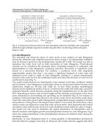
Figure 19a shows the distribution of the friction factor values obtained numerically, for all
simulations performed for the geometrical conditions described in Figure 18a. Figure 19b

Hydrodynamics – Natural Water Bodies

258
contains the distribution of f considering the experimental and the numerical data together.
It was possible to adjust power laws between f and k/h
c
(k=scos), in the form f = a(k/h
c
)
b
.
The values of the adjusted "a" and "b", and the limits of validity of the adjusted equations,
together with the geometrical information, are given in Table 2.


0 0.02 0.04 0.06 0.08 0.1 0.12 0.14
0
5
10
15
f
Pdf


Numerical results
0 0.05 0.1 0.15 0.2 0.25 0.3 0.35

0
2
4
6
8
10
12
f
Pdf


Experimental and numerical res ults

(a) (b)

Fig. 19. Friction factor: (a) Probability distribution function for 11.31º51.13
o
and
numerical results; (b) Probability distribution function considering the numerical
(11.31º51.13
o
) and the experimental results together (=45
o
). The total area covered by
the bars is equal to 1.0 in both figures (R = correlation coefficient; Re = 4q/).



a b
k/h

c

Re R
[degrees] [-] [-] [-] [-] [-]
53.13 0.195 0.502 0.0798-0.485 8.0E6-1.2E8 0.97
45.00 0.146 0.355 0.0776-0.311 2.0E7-1.6E8 0.97
30.96 0.185 0.294 0.0942-0.377 2.0E7-1.6E8 0.96

Table 2. Coefficients for f = a(k/h
c
)
b
and other details.
5. Conclusions
In this chapter different aspects of the flows over stepped spillways were described,
considering analytical, numerical and experimental points of view. The results show
characteristics not usually found in the literature, and point to the need of more studies in
this field, considering the practical use of stepped chutes in hydraulic structures.

Stepped Spillways: Theoretical, Experimental and Numerical Studies

259
6. Acknowledgements
The authors thank CNPq(141078/2009-0), CAPES and FAPESP, Brazilian research support
institutions, for the financial support of this study.
7. References
Arantes, E. J. (2007). Stepped spillways flow characterization using CFD tools. Dr Thesis,
School of Engineering at São Carlos, University of São Paulo, São Carlos, Brazil [in
Portuguese].
Bauer, W.J. (1954). Turbulent boundary layer on steep slopes.

Transactions, ASCE, Vol. 119,
Paper 2719, pp. 1212-1232.
Bernoulli, J. (1743).
Hydraulics. Dover Publications, 2005.
Boes, R. (2000). Zweiphasenströmung und Energieumsetzung an Grosskaskaden. PhD
Thesis – ETH, Zurich.
Boes, R.M. & Hager, W.H. (2003a). Hydraulic Design of Stepped Spillways. ASCE, Journal of
Hydraulic Engineering. v.129, n.9, pp.671-679.
Boes, R.M. & Hager, W.H. (2003b). Two-Phase flow characteristics of stepped spillways.
ASCE,
Journal of Hydraulic Engineering. v.129, n.9, p.661-670.
Bombardelli, F.A.; Meireles, I. & Matos, J. (2010). Laboratory measurements and multi-block
numerical simulations of the mean flow and turbulence in the non-aerated
skimming flow region of steep stepped spillways. Environ. Fluid Mech., v.11, n.3,
pp.263-288. Publisher: Springer Netherlands (DOI 10.1007/s10652-010-9188-6).
Cain, P. & Wood, I.R. (1981) Instrumentation for aerated flow on spillways. ASCE,
Journal of
Hydraulic Engineering, Vol. 107, No HY11.
Carosi, G. & Chanson, H. (2006). Air-water time and length scales in skimming flows on a
stepped spillway. Application to the spray characterization. The University of
Queensland, Brisbane, Austrália.
Carvalho, R.F. & Martins, R. (2009). Stepped Spillway with Hydraulic Jumps: Application of
a Numerical Model to a Scale Model of a Conceptual Prototype.
Journal of Hydraulic
Engineering
, ASCE 135(7):615–619.
Chamani, M.R. & Rajaratnam, N. (1999a). Characteristic of skimming flow over stepped
spillways. ASCE,
Journal of Hydraulic Engineering. v.125, n.4, p.361-368, April.
Chamani, M. R.; Rajaratnam, N. (1999b). Onset of skimming flow on stepped spillways.

ASCE,
Journal of Hydraulic Engineering. v.125, n.9, p.969-971.
Chanson, H. (1993). Stepped spillway flows and air entrainment.
Canadian Journal of Civil
Engineering.
v.20, n.3, p.422-435, Jun.
Chanson, H. (1994). Hydraulics of nappe flow regime above stepped chutes and spillways.
Journal of Hydraulic Research, v.32, n.3, p.445-460, Jan
Chanson, H. (1996).
Air bubble entrainment in free-surface turbulent shear flows. Academic
Press, San Diego, California.
Chanson, H. (2002).
The hydraulics of stepped chutes and spillways. A.A. Balkema Publishers,
ISBN 9058093522, The Netherlands.

Hydrodynamics – Natural Water Bodies

260
Chen, Q.; Dai, G. & Liu, H. (2002). Volume of fluid model for turbulence numerical
simulation of stepped spillway overflow.
Journal of Hydraulic Engineering, ASCE
128(7): pp.683–688.
Cheng X.; Luo L. & Zhao, W. (2004). Study of aeration in the water flow over stepped
spillway. In: Proceedings of the World Water Congress 2004, ASCE, Salt Lake City,
UT, USA.
Chow, V.T. (1959). Open channel hydraulics. New York: McGraw-Hill.
Diez-Cascon, J.; Blanco, J.L.; Revilla, J. & Garcia, R. (1991). Studies on the hydraulic behavior
of stepped spillways.
Water Power & Dam Construction, v.43, n.9, p.22-26, Sept
Frizell, K.H. (2006). Research state-of-the-art and needs for hydraulic design of stepped

spillways.
Water Resources Researches Laboratory. Denver, Colorado, June.
Hager, W.H. (1995).
Cascades, drops and rough channels. In.: Vischer, D.L.; Hager, W.H. (Ed.).
Energy dissipators IAHR, Hydraulics Structures Design Manual. v.9, p.151-165,
Rotterdam, Netherlands.
Essery, I.T.S. & Horner, M.W. (1978). The hydraulic design of stepped spillways. 2nd Ed.
London: Construction Industry Research and Information Association, CIRIA
Report No. 33.
Horner, M.W. (1969). An analysis of flow on cascades of steps. Ph.D. Thesis – Universidade
de Birmingham, UK.
Inoue, F.K. (2005). Modelagem matemática em obras hidráulicas. MSc Thesis, Setor de
Ciências Tecnológicas da Universidade Federal do Paraná, Curitiba.
Keller, R.J.; Lai, K.K. & Wood, I.R. (1974). Developing Region in Self-Aerated Flows.
Journal
of Hydraulic Division
, ASCE, 100(HY4), pp. 553-568.
Keller, R.J. & Rastogi, A.K. (1977). Prediction of flow development on spillway.
Journal of
Hydraulic Division
, ASCE, Vol. 101, No HY9, Proc. Paper 11581, Sept.
Landau, L.D. & Lifshitz, E.M. (1987).
Fluid Mechanics. 2nd Ed. Volume 6 of Course of
Theoretical Physics, ISBN 978-0750627672.
Lobosco, R.J. & Schulz, H.E. (2010). Análise Computacional do Escoamento em Estruturas
de Vertedouros em Degraus.
Mecanica Computacional, AAMC, Vol. XXIX, No 35,
Buenos Aires,
pp.3593-3600.
Lobosco, R.J.; Schulz, H.E.; Brito, R.J.R. & Simões, A.L.A. (2011). Análise computacional

da aeração em escoamentos bifásicos sobre vertedouros em degraus. 6º
Congresso Luso-Moçambicano de Engenharia/3º Congresso de Engenharia de
Moçambique.
Lueker, M.L.; Mohseni, O.; Gulliver, J.S.; Schulz, H.E. & Christopher, R.A. (2008). The
physical model study of the Folsom Dam Auxiliary Spillway System, St. Anthony
Falls Lab. Project Report 511. University of Minnesota, Minneapolis, MN.
Matos, J.S.G. (1999). Emulsionamento de ar e dissipação de energia do escoamento em
descarregadores em degraus. Research Report, IST, Lisbon, Portugal.
Murzyn, F.& Chanson, H. (2009) Free-surface fluctuations in hydraulic jumps: Experimental
observations.
Experimental Thermal and Fluid Science, 33(2009), pp.1055-1064.
Ohtsu, I. & Yasuda, Y. (1997). Characteristics of flow conditions on stepped channels. In:
Biennal Congress, 27, San Francisco, Anais… San Francisco: IAHR, pp. 583-588.

Stepped Spillways: Theoretical, Experimental and Numerical Studies

261
Ohtsu, I., Yasuda Y., Takahashi, M. (2001). Onset of skimming flow on stepped spillways –
Discussion.
Journal of Hydraulic Engineering. v. 127, p. 522-524. Chamani, M.R.;
Rajaratnam, N. ASCE, Journal of Hydraulic Engineering. v. 125, n.9, p.969-971, Sep.
Ohtsu, I.; Yasuda, Y. & Takahashi, M. (2004). Flows characteristics of skimming flows in
stepped channels. ASCE,
Journal of Hydraulic Engineering. v.130, n.9, pp.860-869,
Sept
Peterka, A. J. (1953). The effect of entrained air on cavitation pitting.
Joint Meeting Paper,
IAHR/ASCE, Minneapolis, Minnesota, Aug
Peyras, L.; Royet, P. & Degoutte, G. (1992). Flow and energy dissipation over stepped gabion
weirs.

Journal of Hydraulic Engineering, v.118, n.5, p.707-717, May
Povh, P.H. (2000). Avaliação da energia residual a jusante de vertedouros em degraus com
fluxos em regime skimming flow. [Evaluation of residual energy downstream of
stepped spillways in skimming flows]. MSc Thesis. Department of Technology,
Federal University of Paraná, Curitiba, Brazil [in Portuguese].
Rajaratnam, N. (1990). Skimming flow in stepped spillways.
Journal of Hydraulic Engineering,
v.116, n.4, p. 587-591, April.
Richter, J. P. (1883).
Scritti letterari di Leonardo da Vinci. Sampson Low, Marston, Searle &
Rivington, Londra. In due parti, p.1198 (volume 2, p.236). Available from
<http:// www.archive.org/details/literaryworksofl01leonuoft (16/04/2008).
Rodi, W. (1993).
Turbulence Models and Their Application in Hydraulics. IAHR Monographs,
Taylor & Francis, 3
a
Ed., ISBN-13: 978-9054101505.
Sanagiotto, D.G. (2003). Características do escoamento sobre vertedouros em degraus de
declividade 1V:0.75H [Flow characteristics in stepped spillways of slope 1V:0.75H].
MSc Thesis. Institute of Hydraulic Research, Federal University of Rio Grande do
Sul, Porto Alegre, Brazil, [in Portuguese].
Simões, A.L.A. (2008). Considerations on stepped spillway hydraulics: Nondimensional
methodologies for preliminary design. MSc. Thesis. School of Engineering at São
Carlos, University of São Paulo, Brazil, [in Portuguese].
Simões, A.L.A. (2011). Escoamentos em canais e vertedores com o fundo em degraus:
desenvolvimentos experimentais, teóricos e numéricos. Relatório (Doutorado) –
Escola de Engenharia de São Carlos – Universidade de São Paulo, 157 pp.
Simões, A.L.A.; Schulz, H.E. & Porto, R.M. (2010). Stepped and smooth spillways: resistance
effects on stilling basin lengths.
Journal of Hydraulic Research, Vol.48, No.3, pp.329-

337.
Simões, A.L.A.; Schulz, H.E. & Porto, R.M. (2011). Transition length between water and air-
water flows on stepped chutes. Computational Methods in Multiphase Flow VI,
pp.95-105, doi:10.2495/MPF110081, Kos, Greece.
Sorensen, R.M. (1985). Stepped spillway hydraulic model investigation.
Journal of Hydraulic
Engineering
, v.111, n.12, pp. 1461-1472. December.
Speziale, C.G.; Sarkar, S. & Gatski, T.B. (1991). Modeling the pressure-strain correlation of
turbulence: an invariant dynamical systems approach.
Journal of Fluid Mechanics,
Vol. 227, pp. 245-272.
Stephenson, D. (1991). Energy dissipation down stepped spillways.
Water Power & Dam
Construction
, v. 43, n. 9, p. 27-30, September.