Waves in fluids and solids Part 8 pptx
Bạn đang xem bản rút gọn của tài liệu. Xem và tải ngay bản đầy đủ của tài liệu tại đây (3.22 MB, 25 trang )
Waves in Fluids and Solids
164
(bottom right), 0.09λ
Sch
(middle right) and 0.5λ
Sch
(upper right) above the water/sediment
interface. At all depths the particles follow retrograde elliptical movements. The ellipses are
close to circular in this case since the eccentricity is close to zero. For harder sediment, the
ellipses are more elongated. Figure 4 shows the same plots as in Figure 3 but for the particle
displacements in the bottom. The penetration depth in the solid is larger than the
wavelength of the Scholte wave. At depth z = 0.01λ
Sch
(upper right) the particles follow a
retrograde elliptical movements, while at depth z = 0.09λ
Sch
(middle right) the particle
movement follows a vertical line, and at depth z = 0.5λ
Sch
(middle right) the particle
movement is a prograde ellipse.
Fig. 3. Particle displacements in the water (left) and the particle orbits at depth z = 0.01λ
Sch
(bottom right), 0.09λ
Sch
(middle right) and 0.5λ
Sch
(upper right) for a Scholte wave at a
water/sediment interface. Arrows show the directions of the movement.
Equations (35) show that all the vertical wave numbers are imaginary, and therefore the
signal amplitudes decrease exponentially with increasing distance from the interface. A
consequence of the imaginary vertical wave numbers is that interface waves cannot be
excited by incident plane waves. This can be easily understood by considering the grazing
angle of the wave in the uppermost medium. This angle is expressed as:
0
0
0
cos 1.
p
pp
c
k
cv
(52)
Equation (52) means that the angle θ
0
must be imaginary and, consequently, cannot be the
incident angle of a propagating plane wave. However, the interface waves can be excited by
a point source close to the interface, that is, as a near-field effect.
The interface waves are confined to a narrow stratum close to the interface, which means
that they have cylindrical propagation loss (i.e., 1/r) rather than spherical spreading loss
(i.e., 1/r
2
), as would be true of waves from a point source located in a medium of infinite
extent. Cylindrical spreading loss indicates that, once an interface wave is excited, it is likely
Interface Waves
165
Fig. 4. Particle displacements in the bottom (left) and the particle orbits at depth z = 0.01λ
Sch
(upper right), 0.09λ
Sch
(middle right) and 0.5λ
Sch
(bottom right) for a Scholte wave at a
water/sediment interface. Arrows show the directions of the movement.
to dominate other waves that experience spherical spreading at long distances. This effect is
familiar from earthquakes, where exactly this kind of interface wave, the Rayleigh wave,
often causes the greatest damage.
4. Applications of interface waves
Knowledge of S-wave speed is important for many applications in underwater acoustics and
ocean sciences. In shallow waters the bottom reflection loss, caused by absorption and shear
wave conversion, represents a dominating limitation to low frequency sonar performance.
For construction works in water, geohazard assessment and geotechnical studies the rigidity
of the seabed is an important parameter (Smith, 1986; Bryan & Stoll, 1988; Richardson et al.,
1991; Stoll & Batista, 1994; Dong et al., 2006, WILKEN et al., 2008; Hovem et al., 1991).
In some cases the S-wave speed and other geoacoustic properties can be acquired by in-situ
measurement, or by taking samples of the bottom material with subsequent measurement in
laboratories. In practice this direct approach is often not sufficient and has to be
supplemented by information acquired by remote measurement techniques in order to
obtain the necessary area coverage and the depth resolution.
The next section presents a convenient and cost-effective method for how the S-wave speed
as function of depth in the bottom can be determined from measurements of the dispersion
properties of the seismo-acoustic interface waves (Caiti et al., 1994; Jensen & Schmidt, 1986;
Rauch, 1980).
First the experimental set up for interface wave excitation and reception is presented. Data
processing for interface wave visualization is given. Then the methods for time-frequency
analysis are introduced. The different inversion approaches are discussed. All the presented
methods are applied to some real data collected in underwater and seismic experiments.
Waves in Fluids and Solids
166
4.1 Experimental setup and data collection
In conventional underwater experiments both the source and receiver array are deployed in
the water column. In order to excite and receive interface waves in underwater environment
the source and receivers should be located close, less than one wavelength of the interface
wave, to the bottom. The interface waves can be recorded both by hydrophones, which
measure the acoustic pressure, and 3-axis geophones measuring the particle velocity
components. In most cases an array of sensors, hydrophones and geophones are used. The
spacing between the sensors is required to be smaller than the smallest wavelength of the
interface waves in order to fulfil the sampling theorem for obtaining the phase speed
dispersion. Low frequency sources should be used in order to excite the low frequency
components of the interface waves since the lower frequency components penetrate deeper
into the sediments and can provide shear information of the deeper layers. The recording
time should be long enough to record the slow and dispersive interface waves. Due to the
strong reverberation background and ocean noise the seismic interface waves may be too
weak to be observed even if excited. In order to enhance the visualization of interface waves
one needs to pre-process the data. The procedure includes three-step: low pass filtering for
reducing noise and high-frequency pulses, time-variable gain, and correction of geometrical
spreading (Allnor, 2000).
Figure 5 illustrates an experimental setup for excitation and reception of interface wave
from a practical case in a shallow water (18 m depth) environment. Small explosive charges
were used as sound sources and the signals were received at a 24-hydrophone array
positioned on the seafloor; the hydrophones were spaced 1.5 m apart at a distance of 77 –
111.5 m from the source.
Fig. 5. Experimental setup for excitation and reception of interface waves by a 24-
hydrophone array situated on the seafloor.
The 24 signals received by the hydrophone array are plotted in Figure 6. The left panel
shows the raw data with the full frequency bandwidth. The middle panel shows the zoomed
version of the same traces for the first 0.5 s. The first arrivals are a mixture of refracted and
direct waves. In the right panel the raw data have been low pass filtered, which brings out
the interface waves. In this case the interface waves appear in the 1.0 - 2.5 s time interval
illustrated by the two thick lines. The slopes of the lines with respect to time axis give the
speeds of the interface waves in the range of 40 m/s – 100 m/s with the higher-frequency
components traveling slower than the lower-frequency components. This indicates that the
S-wave speed varies with depth in the seafloor.
77 m
24-hydrophone
Sound source
1.5 m
18 m
Interface Waves
167
Fig. 6. Recorded and processed data of the 24-hydrophone array. Left panel: the raw data
with full bandwidth; Middle panel: zoomed version of the raw data in a time window of 0.0
- 0.5 s. Right panel: low pass filtered data in a time window of 0.5 - 3.0 s.
4.2 Dispersion analysis
There are two classes of methods used for time-frequency analysis to extract the dispersion
curve of the interface waves: single-sensor method and multi-sensor method (Dong et al.,
2006). Single-sensor method, which can be used to study S-wave speed variations as function
of distance (Kritski, 2002), estimates group speed dispersion of one trace at a time from
,
()
g
d
v
dk
(53)
where v
g
is group speed, ω angular frequency, and k(ω) wavenumber. This method requires
the distance between the source and receiver to be known. The Gabor matrix (Dziewonski,
1969) is the classical method that applies multiple filters to single-sensor data for estimating
group-speed dispersion curves. The Wavelet transform (Mallat, 1998) is a more recent
method that uses multiple filters with continuously varying filter bandwidth to give a high-
resolution group-speed dispersion curves and improved discrimination of the different
modes. The sharpest images of dispersion curves are usually found with multi-sensor
method (Frivik, 1998 & Land, 1987), which estimates phase-speed dispersion using multiple
traces and the expression is given by
.
()
p
v
k
(54)
This method assumes constant seabed parameters over the length of the array.
Conventionally, two types of multi-sensor processing methods are used for extracting
phase-speed dispersion curves: frequency wavenumber (f-k) spectrum and slowness-
frequency (p-ω) transform methods (McMechan, 1981). The former method requires
regular spatial sampling, while the latter can be used with irregular spacing.
Waves in Fluids and Solids
168
Alternatively, the Principal Components method (Allnor, 2000), uses high-resolution
beamforming and the Prony method to determine the locations of the spectral lines
corresponding to the interface mode in the wavenumber spectra. These wavenumber
estimates are then transformed to phase speed estimates at each frequency using the
known spacing between multiple sensors.
The low pass filtered data in the right panel in Figure 6 is analyzed by applying Wavelet
transform to each trace to obtain the dispersion of group speed. The dispersion of trace
number 10 is illustrated by a contour plot in Figure 7. The dispersion data are obtained by
picking the maximum values along the each contour as indicated by circles. Only one mode,
fundamental mode, is found in this case within the frequency range of 2.5 Hz – 10.0 Hz. The
corresponding group speed is in the range of 50 m/s - 90 m/s, which gives a wavelength of
5.0 m - 36 m approximately. After each trace is processed, the dispersion curves of the group
speed are averaged to obtain a “mean group speed”, which is subsequently used as
measured data to an inversion algorithm to estimate S-wave speed profile.
Fig. 7. Dispersion analysis showing estimated group speed as function of frequency in the
form of a contour map of the time frequency analysis results. The circles are sampling of the
data.
4.3 Inversion methods
The inverse problem can be qualitatively defined as: Given the dispersion data of the
interface waves, determine the geoacoustic model of the seafloor that will predict the same
dispersion curves. In a more formal way, the objective is to find a set of geoacoustic
parameters
m such that, given a known relation
T
between geoacoustic properties and
dispersion data
d,
() .Τ md
(55)
In general, this problem is nonlinear but we present only a linearized inversion scheme: the
Singular Value Decomposition (SVD) of linear system (Caiti et al., 1996). The seafloor model
is discretized in m layers, each characterized by thickness h
i
, density ρ
i
, P-wave speed c
pi
,
and S-wave speed c
si
. The first simplifying assumption is that the seafloor is considered to
be horizontally homogeneous,
so that the geoacoustic parameters are only a function of
Interface Waves
169
depth in the sediment. The second simplifying assumption is that the dispersion of the
interface wave at the water-sediment interface is only a function of S-wave speed of the
bottom materials and the layering. The other geoacoustic properties are fixed and not
changed during the inversion procedure since the dispersion is not sensitive to these
parameters. These assumptions reduce the number of parameters to be estimated and the
computational effort needed, but do not seriously affect the accuracy of the estimates.
The actual computation of the predicted dispersion of phase/group speed is performed
with a standard Thomson-Haskell integration scheme (Haskell, 1953), which has the
advantage of being fast and economical in terms of computer usage. However, different
codes can be used to generate predictions without affecting the structure of the inversion
algorithm. With the assumptions the model generates the dispersion of phase/group speed
n
p
vR as function of the S-wave speed
m
s
cR
:
,
s
p
Tc v
(56)
where Jacobian
nm
Τ RR
. Depending on the system represented by equation (55) is over-
or underdetermined, its solution may not exist or may not be unique. So it is customary to
look for a solution of (56) in the least square sense; that is, a vector
c
s
that minimizes
2
sp
Tc v . Consider the most common case where m < n; that is, we have more data than
parameters to be estimated. The least-square solution is found by solving the normal
equation:
1
() .
TT
sp
cTTTv
(57)
Here
T
T
is the transpose conjugate of matrix T. By using the SVD to the rectangular matrix T
the solution can be expressed as:
,
T
sp
-1
cWΣ Uv
(58)
11
()
.
T
mm
ip
i
sii
ii
ii
uv
cww
(59)
In equations (57), (58) and (59)
[ ]
TT
TWΣ OU
, U and W are unitary orthogonal matrices
with dimension (n
n) and (mm) respectively and Σ is a square diagonal matrix of
dimension m, with diagonal entries
i
called singular values of T with
1
2
…
m
; O is a
zero matrix with dimension (m
(n-m)); u
i
is the ith column of U and w
j
the jth column of W.
Since the matrix
Σ is ill conditioned in the numerical solution of this inverse problem a
technique called regularization is used to deal with the ill conditioning (Tikhonov &
Arsenin, 1977). The regularized solution is given by:
.
TTT
sp
-1
c(TT+HH)Tv
(60)
H with dimension (mm) is a generic operator that embeds the a priori constraints imposed
on the solution and regularization parameter λ > 0. The detailed discussion on
regularization can be found in (Caiti et al., 1994). The regularized solution is given by
Waves in Fluids and Solids
170
†
,
sp
Tcv
(61)
with
.
TT
†-1 -1
T=W(Σ + Σ (HW) (HW)) U
(62)
The inversion scheme described above is used to estimate S-wave speed profile by inverting
the group-speed dispersion data shown in Figure 7. A 6-layered model with equal thickness
is assumed to represent the structure of the bottom. The layer thickness, P-wave speeds and
densities are kept constant during iterations, but the regularization parameter is adjustable.
The inversion results are illustrated in Figure 8. The upper left panel plots the measured
(circles) and predicted (solid line) group speed dispersion data. The measured data and
predicted dispersion curve agree very well. The eigenvalues and eigenvectors of the
Jacobian matrix
T are plotted in the upper right and bottom right panels respectively. The
eigenvalues to the left of the vertical line are larger than the value of the regularization
parameter λ (the vertical line). The corresponding eigenvectors marked with black shading
constitute the S-wave speed profile. The eigenvectors marked with gray shading give no
contribution to the estimated S-wave speed since their eigenvalues are smaller than the
regularization parameter. The bottom left panel presents the estimated S-wave speed versus
depth (thick line) with error estimates (thin line). The error estimate was generated
assuming an uncertainty of 15m/s in the group speed picked from Figure 7.
Fig. 8. Inversion results. Top left: measured (circles) and predicted (solid line) group speed
dispersion; Top right: eigenvalues of matrix T and the value of the regularization parameter
(vertical line). Bottom right: eigenvectors; Bottom left: estimated S-wave speed (thick line)
and error estimates (thin line).
The estimated S-wave speed is 45 m/s in the top layer and increases to 115 m/s in the depth
of 15 m below the seafloor, which corresponds to one-half of the longest wavelength at 3 Hz.
Interface Waves
171
The errors are smaller in the top layer than that in the deeper layer. This can be explained by
the eigenvalues and the behaviors of the corresponding eigenvectors. The eigenvectors with
larger eigenvalues give better resolution, but penetrate only to very shallower depth, while
the eigenvectors with smaller eigenvalues can penetrate deeper depth, but give relatively
poor resolution.
Finally, we present another example to demonstrate the techniques for estimating S-wave
speed profiles from measured dispersion curves of interface waves (Dong et al., 2006). The
data of this example were collected in a marine seismic survey at a location where the water
depth is 70 m. Multicomponent ocean bottom seismometers with 3-axis geophone and a
hydrophone were used for the recording. The geophone measured the particle velocity
components just below the water-sediment interface. The hydrophones were mounted just
above the interface, and measured the acoustic pressure in the water. The receiver spacing
was 28 m and the distance from the source to the nearest receiver was 1274 m. A set of data
containing 52 receivers with vertical, v
z
, and inline, v
x
, components of the particle velocity
are shown in the left two panels in Figure 9. In order to enhance the interface waves the
recorded data are processed by low-pass filtering, time-variable gain and correction of
geometrical spreading (Allnor, 2000). The processed data are plotted in the two right panels
in Figure 9 where the slow and dispersive interface waves are clearly observed. The thick
lines bracket the arrivals of the interface waves. The slopes of the lines with respect to the
time-axis define the speeds of the interface waves. In this case the speeds appear to be in the
range of 290 m/s - 600 m/s for the v
z
component and 390 m/s - 660 m/s for the v
x
component. The higher speed of v
x
component is a consequence of the fact that the v
x
component has weaker fundamental mode and stronger higher-order mode than v
z
component, as can be observed in Figure 10.
Fig. 9. Raw and processed data. From the left to the right: v
z
and v
x
components of raw and
processed data. The thick lines in the processed data illustrate the arrivals of the interface
waves and the slopes of the lines indicate the speed range of the interface waves.
The Principal Components method is applied to the processed data to obtain the phase
speed dispersion. The extracted dispersion data of v
z
(blue dots) and v
x
(red dots) are plotted
in Figure 10. The advantage by using multi-component data is that one can identify and
Waves in Fluids and Solids
172
separate different modes and obtain higher resolution. By combining both v
z
and v
x
dispersion data the final dispersion data are extracted and denoted by circles. There are four
modes identified, but only the first two modes are used in the inversion algorithm for
estimating the S-wave speed. Figure 10 shows that the lower frequency components of the
higher-order mode have higher phase speed and therefore longer wavelength than that the
higher frequency components of the lower-order mode have. In this case the phase speed of
the first-order mode at 2 Hz is 550 m/s, which gives a wavelength of 270 m. A 12-layered
model is assumed to represent the structure of the bottom with layer thickness increasing
logarithmically with increasing depth. The layer thickness, P-wave speeds and densities are
kept constant during iterations, but the regularization parameter is adjustable.
The inversion results are illustrated in Figure 11. The left panel shows the measured phase
speed dispersion data (circles) and the predicted (solid line) phase speed dispersion curve.
The right panel presents the estimated S-wave speed versus depth (thick line) with error
estimates (thin line). The error estimates were generated assuming an uncertainty of 15m/s
in the selection of phase speed from Figure 10. The match between the predicted and
measured dispersion data is quite good for both the fundamental and the first-order modes.
The estimated S-wave speed is 237 m/s in the top layer and increases up to 590 m/s in the
depth of 250 m below the seafloor, which is approximately one of the longest wavelength at
the frequency of 2.0 Hz. The results from the both examples indicate that the Scholte wave
sensitivity to S-wave speed versus depth using multiple modes is larger than that using only
fundamental mode.
Fig. 10. Phase-speed dispersion of v
z
(blue) and v
x
(red) components. The circles are the
sampling of the data.
Over the years considerable effort has been applied to interface-wave measurement, data
processing, and inversion for ocean acoustics applications (Rauch, 1980; Hovem et al., 1991;
Richardson, 1991; Caiti et al., 1994; Frivik et al., 1997; Allnor, 2000; Godin & Chapman, 2001;
Chapman & Godin, 2001; Dong et al, 2006; Dong et al., 2010). Nonlinear inversion gives both
quantitative uncertainty estimation and rigorous estimation of the data error statistics and of
an appropriate model parameterization, and is not discussed here. The work on nonlinear
inversion can be found in Ivansson et al. (1994), Ohta et al. (2008) and Dong & Dosso (2011).
More recently Vanneste et al. (2011) and Socco et al. (2011) used a shear source deployed on
Interface Waves
173
Fig. 11. Inversion results. Left: measured (circles) and predicted (solid line) phase speed
dispersion data; Right: estimated S-wave speed versus depth (thick line) and the error
estimates (thin line).
the seafloor to generate both vertical and horizontal shear waves in the seafloor. This
enabled to measure both Scholte and Love waves and to inverse S-wave speed profile
jointly, thereby obtaining information on anisotropy in the subsurface. Another and entirely
different approach is based on using ocean ambient noise recorded by ocean bottom cable to
extract information on the ocean subsurface. This approach has attracted much attention as
being both economical and environmental friendly (Carbone et al., 1998; Shapiro et al., 2005;
Bensen et al., 2007; Gerstoft et al., 2008; Bussat & Kugler, 2009; Dong et al., 2010).
5. Conclusions
In this chapter after briefly introducing acoustic and elastic waves, their wave equations and
propagation, a detailed presentation on interface waves and their properties is given. The
experimental set up for excitation and reception of interface waves are discussed. The
techniques for using interface waves to estimate the seabed geoacoustic parameters are
introduced and discussed including signal processing for extracting dispersion of the
interface waves, and inversion scheme for estimating S-wave speed profile in the sediments.
Examples with both hydrophone data and ocean bottom multicomponent data are analyzed
to validate the procedures. The study and approaches presented in this chapter provide
alternative and supplementary means to estimate the S-wave structure that is valuable for
seafloor geotechnical engineering, geohazard assessment, seismic inversion and evaluation
of sonar performance.
The work presented in this chapter is resulted from the authors’ number of years of teaching
and research on underwater acoustics at the Norwegian University of Science and
Technology.
6. Acknowledgment
The authors would like to give thanks to Professor N. Ross Chapman, Professor Stan E.
Dosso at the University of Victoria and our earlier colleague Dr. Rune Allnor for helpful
discussions and collaboration.
Waves in Fluids and Solids
174
7. References
Allnor, R. (2000). Seismo-Acoustic Remote Sensing of Shear Wave Velocities in Shallow Marine
Sediments, PhD. Thesis, No. 420006, Norwegian University of Science and
Technology, Trondheim, Norway
Brekhovskikh, L. M. (1960). Waves in Layered media, Academic Press, New York, N. Y. USA
Bryan, G. M. & Stoll, R. D. (1988). The Dynamic Shear Modulus of Marine Sediments, J.
Acoust. Soc. Am., Vol. 83, pp. 2159-2164
Bucker, H. P. (1970). Sound Propagation in a Channel with Lossy Boundaries, J. Acoust. Soc.
Am. Vol. 48, pp. 1187-1194
Bussat, S. & Kugler, S. (2009). Recording Noise - Estimating Shear-Wave Velocities:
Feasibility of Offshore Ambient- Noise Surface Wave Tomography (ANSWT) on a
Reservior Scale, SEG Expanded Abstracts, pp. 1627-1631
Caiti, A., Akal, T. & Stoll, R.D. (1994). Estimation of Shear Wave Velocity in Shallow Marine
Sediments, IEEE J. Ocean. Eng., Vol. 19, pp. 58-72
Carbone, N. M., Deane, G. B. & Buckingham, M. J. (1998). Estimating the compressional and
shear wave speeds of a shallow water seabed from the vertical coherence of
ambient noise in the water column, J. Acoust. Soc. Am., Vol. 103(2), pp. 801-813
Chapman, D. M. F. & Godin, O. A. (2001). Dispersion of Interface Waves in Sediments with
Power-Law Shear Speed Profile. II. Experimental Observations and Seismo-
Acoustic Inversion, J. Acoust. Soc. Am., Vol. 110, pp. 1908-1916
Dong, H., Allouche, N., Drijkoningen, G. G. & Versteeg, W. (2010). Estimation of Shear-
Wave Velocity in Shallow Marine Environment, Proc. of the 10th European Conference
on Underwater Acoustics, Vol. 1, pp. 175-180, Akal, T (Ed.)
Dong, H, Hovem, J. M. & Kristensen, Å. (2006). Estimation of Shear Wave Velocity in
Shallow Marine Sediment by Multi-Component Seismic Data: a Case Study, Procs.
of the 8th European Conference on Underwater Acoustics, Vol. 2, pp. 497-502, Jesus, S.
M. & Rodringuez, O. C. (Ed.)
Dong, H., Hovem, J. M. & Frivik, S. A. (2006). Estimation of Shear Wave Velocity in Seafloor
Sediment by Seismo-Acoustic Interface Waves: a Case Study for Geotechnical
Application, In: Theoretical and Computational Acoustics, pp. 33-43, World Scientific
Dong, H., Liu, L., Thompson, M. & Morton, A. (2010). Estimation of Seismic Interface Wave
Dispersion Using Ambient Noise Recorded by Ocean Bottom Cable, Proc. of the 10th
European Conference on Underwater Acoustics, Vol.
1, pp. 183-188, Akal, T. (Ed.)
Dong, H. & Dosso S. E. (2011). Bayesian Inversion of Interface-Wave Dispersion for Seabed
Shear-Wave Speed Profiles, IEEE J. Ocean. Eng., Vol. 36 (1), pp. 1-11
Dziewonski, A.S., Bloch, S. & Landisman, M. A. (1969). A technique for the analysis of
Transient Seismic Signals, Bull. Seismol. Soc. Am. Vol. 59, pp. 427-444
Frivik, S. A., Allnor, R. & Hovem, J. M. (1997). Estimation of Shear Wave Properties in the
Upper Sea-Bed Using Seismo-Acoustical Interface Waves, In: High Frequency
Acoustics in Shallow Water, pp. 155-162, N. G. Pace, E. Pouliquen, O Bergem, &
Lyons, A. P. (Ed.), NATO SACLANT Undersea Research Centre, Italy
Gerstoft, P., Hodgkiss, W. S., Siderius, M., Huang, C. H. & Harrison, C. H. (2008). Passive
Fathometer Processing, J. Acoust. Soc. Am., Vol. 123, No. 3, pp. 1297-1305
Godin, O. A. & Chapman, D. M. F. (2001). Dispersion of Interface Waves in Sediments with
Power-Law Shear Speed Profile. I. Exact and Approximate Analytic Results, J.
Acoust. Soc. Am., Vol. 110, pp. 1890-1907
Interface Waves
175
Haskell, N. A. (1953). Dispersion of Surface Waves on Multilayered Media, Bullet. Seismolog.
Soc. of America, Vol. 43, pp. 17-34
Hovem, J. M. (2011). Marine Acoustics: The Physics of Sound in Underwater Environments,
Peninsula Publishing, ISBN 978-0-932146-65-6, Los Altos Hills, California, USA.
Hovem, J. M., Richardson, M. D. & Stoll, R. D. (1991), Shear Waves in Marine Sediments,
Dordrecht: Kluwer Academic
Ivansson, S., Moren, P. & Westerlin, V. (1994). Hydroacoustical Experiments for the
Determination of Sediment Properties, Proc. IEEE Oceans94, Vol. III, pp. 207-212
Jensen, F. B., & Schmidt, H. (1986). Shear Properties of Ocean Sediments Determined from
Numerical Modelling of Scholte Wave Data, In: Ocean Seismo-Acoustics, Low
Frequency Underwater Acoustics, Akal, T. & Berkson, J. M. (Ed.), pp. 683-692, Plenum
Press, New York, USA
Kritski, A., Yuen, D.A. and Vincent, A. P. (2002). Properties of Near Surface Sediments from
Wavelet Correlation Analysis, Geophysical Research letters, Vol. 29, pp. 1922-1925
Land, S. W., Kurkjian, A. L., McClellan, J. H., Morris, C. F. & Parks, T. W. (1987). Estimating
Slowness Dispersion from Arrays of Sonic Logging Waveforms”, Geophysics, Vol.
52 No. 4, pp. 530-544
Love, A. E. H. (1926). Some Problems of Geodynamics, 2
nd
ed. Cambridge University Press,
London
Mallat, S. (1998). A Wavelet Tour of Signal Processing, Academic Press, USA
McMechan, G. A. & Yedlin, M. J. (1981). Analysis of Dispersion Waves by Wave-Field
Transformation, Geophysics, Vol. 46, pp. 869-874
Ohta, K., Matsumoto, S., Okabe, K., Asano, K. & Kanamori, Y. (2008). Estimation of Shear-
Wave Speed in Ocean-Bottom Sediment Using Electromagnetic Induction Source,
IEEE J. Ocean. Eng., Vol. 33, pp. 233-239
Rauch, D. (1980). Seismic Interface Waves in Coastal Waters: A Review, SACLANTCEN Report
SR-42, NATO SACLANTASW Research Centre, Italy
Richardson, M. D., Muzi, E., Miaschi, B. & Turgutcan, F. (1991). Shear Wave Velocity
Gradients in Near-Surface Marine Sediments, In: Shear Waves in Marine Sediments,
Hovem, J. M., Richardson, M. D. & Stoll, R. D., (Ed.), pp. 295-304, Dordrecht:
Kluwer Academic
Shapiro, N. M., Campillo, M., Stehly, L. & Ritzwoller, M. H. (2005). High Resolution Surface
Wave Tomography from Ambient Seismic Noise, Science, Vol. 307, pp. 1165-1167
Smith, D. T. (1986). Geotechnical Characteristics of the Seabed Related to Seismo-Acoustics,
In: Ocean Seismo-Acoustics, T. Akal and J. M. Berkson, (Ed.), PP. 483-500, Plenum,
New York, USA
Socco, V. L., Boiero, D., Maraschini, M., Vanneste, M., Madshus, C., Westerdahl, H., Duffaut,
K. & Skomedal, E. (2011). On the use of the Norwegian Geotechnical Institute’s
prototype seabed-coupled shear wave vibrator for shallow soil characterization –
II. Joint inversion of multimodal Love and Scholte surface waves, Geophys. J. Int.,
Vol. 185 (1), pp. 237-252
Stato, Y. (1954). Study on Surface waves XI. Definition and Classification of Surface Waves,
Bulletin, Earthquake Research Institute, Tokyo University, Vol. 32, pp. 161-167
Stoll, R. D. & Batista, e. (1994). New Tools for Studying Seafloor Geotechnical Properties, J.
Acoust. Soc. Am., Vol. 96, pp. 2937-2944
Tikhonov, A. N. & Arsenin,V. Y. (1977). Solution of Ill-Posed Problems, New York Wiley, USA
Waves in Fluids and Solids
176
Viktirov, I. A. (1967). Rayleigh and Lamb Waves, Plenum Press, New York, N. Y. USA
Vanneste, M., Madshus, C., Socco, V.L., Maraschini, M., Sparrevik, P. M., Westerdahl, H.,
Duffaut, K., Skomedal, E. & Bjørnarå, T. I. (2011). On the use of the Norwegian
Geotechnical Institute’s prototype seabed-coupled shear wave vibrator for shallow
soil characterization – I. Acquisition and processing of multimodal surface waves,
Geophys. J. Int., Vol. 185 (1), pp. 221-236
Westwood, E. K.; Tindle, C. T. & Chapman, N. R. (1996). A Normal Mode Model for
Acousto-Elastic Ocean Environments, J. Acoust. Soc. Am. Vol. 100, pp. 3631-3645
Wilken, D., Wolz, S., Muller, C. & Rabbel, W. (2008). FINOSEIS: A New Approach to
Offshore-Building Foundation Soil Analysis Using High Resolution Seismic
Reflection and Scholte-Wave Dispersion Analysis, J. Applied Geophysics, Vol. 68, pp.
117-123
7
Acoustic Properties of the
Globular Photonic Crystals
N. F. Bunkin
1
and V. S. Gorelik
2
1
A.M.Prokhorov General Physics Institute, Russian Academy of Sciences,
2
Lebedev Physical Institute, Russian Academy of Sciences,
Moscow,
Russia
1. Introduction
Modern technologies allow us to construct new nanomaterials with a periodic
superstructure. In particular, the increasing interest has been recently shown in the so-called
photonic (PTC) [1 - 4] and phononic (PNC) [5] crystals. In a case of PTC its structure is
characterized by the refractive index, which periodically varies in space; the spatial period
essentially exceeds the atomic sizes. PNCs are characterized by spatial periodic modulations
of the sound velocity caused by the presence of the periodically settled elements of various
materials (metals, polymers etc.) inside the sample. It is worth noting that PTC can at the
same time be treated as a version of PNC.
PTCs and PNCs can be realized as one, two and three-dimensional structures. Among a
wide variety of PTCs the special attention of researchers is paid to the crystal structures,
whose lattice period is comparable with a wavelength of electromagnetic wave in the visible
range. The periodicity of such PTC-structure results in presence of the so-called band-gaps
located in the visible spectral range, i.e. in the spectral areas, where the electromagnetic
waves can penetrate inside the sample only to a near-surface region with thickness of about
a wavelength of light (0.4-0.8 microns). If the frequency of an electromagnetic wave is close
to the band-gap edge, the group velocity of an electromagnetic wave drastically decreases,
which results in a sharp increase of spectral density of electromagnetic radiation [2]. The
numerous works are devoted to study of such effect for the visible range [2 - 4]. Other
interesting feature of PTC consists in the existence of spectral bands characterized by a
negative value of the effective refractive index, when the directions of phase and group
velocities of an electromagnetic wave appear to be opposite to one another. At last we shall
note that effective rest mass of photons in PTC is non-zero and can accept both positive and
negative values. The absolute value of the effective rest mass of the photons in PTC is equal
to
36
2
10m
c
ω
−
=≈
kg.
The properties of acoustic waves in PNC are in many respects similar to the properties of
electromagnetic waves in PTC. In the given work the review of characteristic properties of
acoustic waves in PNC in comparison with the corresponding properties of electromagnetic
waves in PTC is given. In particular, the problems of finding the form of dispersion
dependences ω(k) for acoustic waves together with the dispersion dependences of their
Waves in Fluids and Solids
178
group velocities and effective mass of the corresponding acoustic phonons are solved. The
results of the theoretical analysis and the data of experimental studies of the optical and
acoustic phenomena in PTC and PNC, including the studies of spectra of non-elastic
scattering of light together with the experiments to observe the stimulated light scattering
accompanying by the coherent oscillations of globules are reported.
1.1 Theory of dispersion of electromagnetic and acoustic waves in one-dimensional
PTC/PNC
The one-dimensional dielectric medium with two alternating layers (see. Fig. 1) can be
considered as a one-dimensional PTC. At the same time, such medium can either be
regarded as a one-dimensional PNC characterized by specified propagation velocities of
acoustic waves in each of layers. At the first stage, let us consider the dispersion law for
electromagnetic waves on the basis of the theory developed earlier [5 - 7]. According to the
technique described in detail in Ref. [5], in order to obtain the dispersion relation, we used
the plane monochromatic wave approximation with allowance for the boundary conditions
at the edges of the layers (see Fig. 1).
Fig. 1. Schematic of periodic layered medium and plane wave amplitudes corresponding to
the n-th unit cell and its neighboring layers [5]
The periodic layered medium under study consists of two various substances with the
following structure of the refractive index:
()
Λ<<
<<
=
,,
,0,
1
2
zbn
bzn
zn
(1)
With making allowance for the periodicity of the refractive index, we arrive at:
() ( )
.Λ+= znzn
(2)
Here the z-axis is perpendicular to the boundaries of layers, while Λ is the spatial period of
the superstructure. The general solution to the wave equation for the electric field vector can
be sought for in the form
Acoustic Properties of theGlobular Photonic Crystals
179
() ()
()
0
,exp .
y
tzitky
ω
=−
Er E
(3)
Here it is assumed that the wave propagates in (yz) plane, whereas k
y
is the vector
component that remains constant during the propagation through the medium. The electric
field strength within each homogeneous layer can be represented as a sum of the incident
and reflected plane waves. Complex amplitudes of these two waves are components of the
column vector. Thus, the electric field in
α
-th layer (
α
= 1, 2) of the n-th unit cell (see. Fig. 1)
can be written in the form of the column vector
()
()
,1,2.
n
n
a
b
α
α
α
=
(4)
The distribution of the electric field strength in the layer under consideration can be
represented as
()
()
()
()
()
{
}
()
,exp exp exp,
nz nz y
Eyz a ik z n b ik z n iky
αα
αα
= −−Λ + −−Λ −
(5)
where
2
2
,1,2.
zy
n
kk
c
α
α
ω
α
=− =
(6)
The column vectors are related to each other by the conditions of continuity at the interfaces.
As a consequence, only one vector (or two components of different vectors) can be chosen
arbitrarily. For TE-waves (vector Е is perpendicular to the yz plane), the condition for the
continuity of the components E
x
and H
y
(H
y
~ ∂E
x
/∂z) [6, 7] at the interfaces z = (n –1)Λ and z
= (n – 1)
Λ + b (see Fig. 1) leads to the following equations:
()
()
()()
22 22
2211 22 11
11 1112
21
,,
,.
zz zz
zzzz zz zz
ik ik ik ik
nn n nznn z n n
ik a ik a ik a ik a ik a ik a ik a ik a
nnnnznnznn
a b ece dika b ikece d
ecedeaebikeced ikeaeb
Λ−Λ Λ−Λ
−− −−
−− − −
+= + − = −
+=+ + = +
(7)
These four equations can be written as a system of two matrix equations:
() ( )
() ()
22
1
22
22
1
11
exp exp
11
,
exp exp
11
zz
n n
zz
zz
n n
zz
ik ik
ac
kk
ik ik
bd
kk
−
−
Λ−Λ
⋅= ⋅
Λ− −Λ
−
(8)
() ( )
() ( )
() ( )
() ()
11
22
11
11
22
22
exp exp
exp exp
,
exp exp
exp exp
zz
nn
zz
zz
zz
nn
zz
zz
ik a ik a
ca
ik a ik a
kk
ik a ik a
db
ik a ik a
kk
−
−
⋅= ⋅
−−
−−
(9)
where
Waves in Fluids and Solids
180
() () () ()
1122
,,,.
nn nn nn nn
aa bb ca db≡ ≡ ≡ ≡ (10)
Eliminating the column vector (c
n
, d
n
)
T
from this system, we obtain the matrix equation
1
1
.
nn
nn
aABa
bCDb
−
−
=
(11)
The matrix elements in this equation are:
() ()
() ()
21 21
12 2 1 2
12 12
21 21
1212
12 12
11
exp cos sin , exp sin ,
22
11
exp sin , exp cos
22
zz zz
zz z z z
zz zz
zz zz
zzzz
zz zz
kk kk
A ika kb i kb B ika i kb
kk kk
kk kk
Cikai kbD ikakbi
kk kk
=⋅++ =−⋅−
=⋅−− =−⋅−+
2
sin .
z
kb
(12)
Since the matrix (11) relates amplitudes of the field of two equivalent layers with identical
refractive indices, it is unimodular, i.e.,
AD – BC = 1 (13)
As was pointed out above, only one column vector is independent. For this vector one can
choose, for instance, the column vector for layer 1 in the zero unit cell. The remaining
column vectors of the equivalent layers are connected with the vector for the zero unit cell
by the relation
0
0
.
n
n
n
aABa
bCDb
=
(14)
It follows from here that
0
0
,
n
n
n
aABa
bCDb
−
=
(15)
or, in view of (14)
0
0
.
n
n
n
aDBa
bCAb
−
=
−
(16)
A periodic layered medium is equivalent to a one-dimensional PTC that is invariant under
translations to the lattice constant. The lattice translation operator T is defined by the
expression
,Tz z l=−Λ
l ∈ Z.
Thus, we arrive at
()
()
()
1
.Tz Tz zl
−
==+ΛEE E (17)
Acoustic Properties of theGlobular Photonic Crystals
181
According to the Bloch theorem [6, 7], the vector of the electric field of the normal mode in
the layered periodic medium has the form:
() ( )
()
exp exp ,
Ky
ziKzitky
ω
=− −
EE
(18)
where E
K
(z) is the periodic function with the period Λ, i.e.,
() ( )
.
KK
zz=+ΛEE (19)
Using the column vector representation and expression (5), the periodicity condition (19) for
the Bloch wave can be written as:
()
1
1
exp .
nn
nn
aa
iK
bb
−
−
=−Λ
(20)
As follows from Eqns. (11) and (20), the column vector of the Bloch wave obeys the
eigenvalue equation:
()
exp .
nn
nn
AB a a
iK
CDb b
=Λ
(21)
Thus, the phase factor is the eigenvalue of the translation matrix (A B C D) and satisfies the
characteristic equation
()
()
exp
det 0.
exp
AiK B
CDiK
−Λ
=
−Λ
The solution to this equation has the form
()()()
2
11
exp 1.
22
iK A D A DΛ= + ± + − (22)
Eigenvectors corresponding to these eigenvalues are solutions to Eqn. (21), and accurate to
an arbitrary constant they can be represented in the form
()
0
0
exp
B
a
iK A
b
=
Λ−
(23)
According to (20), the corresponding column eigenvector for the n-th unit cell is
()
()
exp .
exp
n
n
B
a
inK
iK A
b
=−Λ
Λ−
(24)
The Bloch waves obtained from (23) and (24) can be considered as eigenvectors of the
translation matrix with the eigenvalues exp(iKΛ), given by Eqn. (22); this equation results in
the dispersion relation of the kind:
Waves in Fluids and Solids
182
()
1
,arccos .
2
y
AD
Kk
ω
+
=
Λ
(25)
The modes, in which |A + D|/2 < 1, correspond to the real K. If |A + D|/2 < 1, the relation
K = m
π
/λ + iK
m
takes place, i.e., the imaginary part in the wave vector K is non-zero, and the
wave is damped. Thus the so-called band-gap opens. The frequencies corresponding to the
band-gap boundaries are found from the condition
/2 1.AD+=
At normal incidence (k
y
=0), the dispersion dependence ω(K) has, according to (25), the
following form:
() ()() ()()
21
12 12
12
1
cos cos cos sin sin .
2
nn
Kkakb kakb
nn
Λ= − +
(26)
The quantities in Eqn. (26) have the following physical meaning: i = 1 is the subscript related
to the first medium, while i = 2 is the subscript related to the second medium; n
1
= n
1
(ω) is
the refractive index of the first medium, and n
2
= n
2
(ω) is the refractive index of the second
medium;
(1 )a
η
=−Λ, b
η
=Λ, η is the content of the second medium in the layered PTC;
()
0
i
i
n
k
C
ω
ω
⋅
=
is the wave vector in the i-th medium, and С
0
= 3·10
8
m/s is the velocity of
light in vacuum.
As the first approximation we can assume that the refractive index values of both layers
n
1
and
n
2
are the constant values and do not depend on the electromagnetic radiation
frequency. At the next stage we shall take into account their dependence on the frequency
(or on the wavelength of a radiation illuminating the PTC). For example, let us consider a
one-dimensional PTC, one layer of which is amorphous quartz (SiO
2
), and second layer is
atmospheric air, for which the refractive index is ~ 1. Additionally, we will consider that the
refractive index of SiO
2
is not dependent upon the wavelength, i.e. n
1
= 1.47. Finally, we will
use the following values of the parameters
a
1
and a
2
: specifically, а
1
= 136 nm, and а
2
= 48
nm. In this case the dispersion law for the electromagnetic waves in PTC can be obtained by
using Eqn. (26). The results of numerical simulation of the dispersion curves
()k
ω
(these
curves were taken from our study [8]) are plotted in Fig. 2 by the bold lines. As is seen from
this Figure, we can discern in the spectrum three dispersion branches ( ), ( 1,2,3),
j
kj
ω
=
where the first one is related to the low-frequency range, including the infra-red spectral
area, the second one is related to the visible spectral range, and the third one is related to the
near ultra-violet spectrum. The additional branches are plotted in view of anomalous
dispersion of the refractive index at approaching the electronic absorption band in SiO
2
. In
Fig. 2 two photonic band-gaps, where the first one corresponds to the Brillouin zone
boundary (
k
π
=
Λ
), and the second one is related to the Brillouin zone center (k = 0), are
seen. The second dispersion branch is related to the case, where the directions of the phase
and group velocities are opposite with respect to one another, i.e. to the case of negative
effective refractive index
(0)n < .
As was found in study [8], the good enough description of the dispersion curves (see the
gray curves (2) in Fig. 2, which were plotted on the basis of the exact theory given by Eqn.
(26)), can be carried out by using the approximated formulas of the kind:
Acoustic Properties of theGlobular Photonic Crystals
183
0
1
2sin ,
2
Ck
m
ω
Λ
=
Λ
- the first dirpersion branch, (27)
2
22 2
0
2
2
2sin
2
Ck
m
ωω
Λ
=−
Λ
- the second dirpersion branch, (28)
2
22 2
0
3
3
2sin
2
Ck
m
ωω
Λ
=+
Λ
- the third dirpersion branch. (29)
Here
ω
1
and
ω
2
are the frequencies corresponding to the edges of the second order band-
gap, m
1
, m
2
, and m
3
are the effective refractive indices for the first, the second and the third
dispersion branches accordingly. The following values for the frequencies and refractive
indices were taken: ω
2
= 3.62⋅10
15
radian/s,
ω
2
= 3.62⋅10
15
radian/s,
ω
3
=4.14⋅10
15
radian/s,
and m
1
= 0,94; m
2
= 0.555; m
3
= 0.435. Besides, the opportunity of approximating the
dispersion curves close to the center of the Brillouin zone by the so-called quasi-relativistic
formulas (30) – (33) was considered:
0
1
C
k
m
ω
= - the first dirpersion branch, (30)
2
22 2
0
2
2
C
k
m
ωω
=−
- the second dirpersion branch, (31)
2
22 2
0
3
3
C
k
m
ωω
=+
- the third dirpersion branch, (32)
0 2 4 6 8 10 12 14 16 18
0
2
4
6
8
10
12
K,10
6
1/m
ω,
10
15
rad/s
1
2
1
2
Fig. 2. The dispersion law
ω
(k) for a one-dimensional PTC; (1) - the results of calculation of
the dispersion dependence ω(k) according to (26), (2) – the results of calculation of the
dispersion dependence ω(k) with the help of sinusoidal approximation.
Waves in Fluids and Solids
184
024681012141618
0
2
4
6
8
10
12
K, 10
6
1/m
ω,
10
15
rad/s
3
1
1
3
Fig. 3. The dispersion law
ω
(k) for a one-dimensional PTC; (1) - the results of calculation of
the dispersion dependence ω(k) according to (26), (3) – the results of calculation of the
dispersion dependence ω(k) with the help of quasi-relativistic approximation.
As is seen from Fig. 3, the satisfactory agreement between the curves 1 and 3 takes place
only at small values of a wave vector (i.e., close to the center of the Brillouin zone).
Nonetheless, this approach allows us to estimate the effective photonic mass basing on the
equality (here m
0
and Е
0
are the effective rest mass and the rest energy of the photon.)
0
22
22
22
1(0)(0)
;.
E
mm
dE d
CC
dp dk
ω
ω
== ==
(33)
For the second dispersion branch the effective rest mass of the photon appears to be
negative and equal to
35
1
2
2
0
2
2
0,13 10m
C
m
ω
−
=− =− ⋅
kg. Accordingly for the third branch we
obtain:
35
2
3
2
0
2
3
0,09 10m
C
m
ω
−
==⋅
kg. Thus, the effective rest mass of a photon inside the PTC
appears to be non-zero and can acquire both positive and negative magnitudes.
If one takes into account the dispersion of refractive index for the layers, forming PTC, the
dispersion law
()k
ω
can also be received from numeric solution to Eqn. (26). For example,
let us consider PTC, where the first medium is SiO
2
, whereas the second medium is
atmospheric air or water. The refractive index of air is assumed to be equal to unity. Thus
for the dependence of the SiO
2
refractive index versus a wavelength we can use the formula:
222
2
1
222222
0,6962 0,4079 0,8975
1,
0,0684 0,1162 9,896
n
λλλ
λλλ
−= + +
−−−
while the same dependence for water is given by the formula:
12 12 22 12
2
2
23222221
5,667 10 1,732 10 2,096 10 1,125 10
1
5,084 10 1,818 10 2,625 10 1,074 10
n
λλλλ
λλλλ
−−−−
−−−
⋅⋅⋅⋅
−= + + +
−⋅ −⋅ −⋅ −⋅
Acoustic Properties of theGlobular Photonic Crystals
185
(a)
(b)
Fig. 4. The calculated dispersion curves; (а) – the initial PTC; (b) – the PTC, filled with water.
The band-gap boundaries (thin solid lines), the edge of the first Brillouin zone together with
the straight line indicating the dispersion law for a light wave in vacuum (ω = С
0
·k) are
indicated.
The calculated dispersion curves for these cases are shown in Fig. 4 (a) and (b). As is seen in
this Figure, implantation of water instead of air in PTC results in decreasing the optical
contrast and, accordingly, in reducing the band-gap width for the visible and ultraviolet
spectral ranges. Accounting for the dispersion of the refractive index for SiO
2
results in
occurrence of the additional dispersion branch in the infrared spectral range; this branch is
related to the polariton curve, stimulated by the polar vibrations, e.g., the vibrations along the
bond Si-O in the microstructure of quartz. In Fig. 4 the points of intersection of the straight
line, corresponding to the light wave (this line is set by the formula ω = С
0
·k, for which the
effective refractive index is equal to unity) are marked. Thus according to the known Fresnel
formulas the reflectance of a light wave from the PTC interface approaches zero, and the
material should become absolutely transparent (provided that the absorption is absent).
1.2 Calculation of the dispersion characteristics for the one-dimensional PNC
As was already noted, PNC can either be considered as PTC with making allowance for the
fact that the sonic wave velocities depend upon the type of material of a layer. Using the
Waves in Fluids and Solids
186
optical-acoustic analogy for describing the dispersion of acoustic waves in PNC and basing
upon Eqn. (26), we obtain the following dispersion equation for the acoustic wave
propagating in PNC along the crystallographic direction (111):
() ( ) ( ) () ()
22
12
11 22 11 22
12
1
cos cos cos sin sin .
2
VV
ka ka ka ka ka
VV
+
=⋅− ⋅
⋅
(34)
The quantities entering into (34) have the following physical meaning: i = 1 is the subscript
for SiO
2
(opal matrix); i = 2 is the subscript for the layer, filled with a metal or liquid; V
1
is
the velocity of acoustic waves in opal; V
2
is the velocity of sound in the medium that fills the
pores in the opal (see table 1); η = 0,26 is the effective sample porosity coefficient, D = 220
nm is the diameter of the quartz globules;
2
3
aD=
is the period of the structure of the opal
samples under investigation;
a
1
= (1 – η)a, a
2
= ηa; ω
i
is the cyclic frequency of the acoustic
wave;
()
/
ii
kv
ωω
= is the wave vector in the i-th medium.
Material
Transverse wave velocity, km
⋅s
-1
Longitudinal wave velocity, km⋅s
-1
Opal 3.3 5.3
Air 0.1 0.3
Water 0.6 1.5
Gold 1.2 3.2
Table 1. Velocities of longitudinal and transverse acoustic waves
Based on the numerical analysis of (34), we constructed the dispersion dependences
()k
ω
for
different branches in the acoustic region of the spectrum. The numerically simulated
acoustic properties of various PNCs are shown in Fig. 5.
The abscissas are the wave vector values, scaled in m
-1
, and the ordinates are the cyclic
frequencies (rad
⋅s
-1
); the solid lines indicate longitudinal waves and the dashed lines
indicate transverse waves. Fig. 5 (a) corresponds to the initial (unfilled) opal containing air
in its pores, whereas Fig. 5 (b) shows the dispersion dependence
()k
ω
for the sample with
water in its pores, and Fig. 5 (c) displays acoustic branches of PTC with nanoparticles of
gold. As is seen from these graphs, both in PTC and PNC the band-gaps are being formed,
whose location and bandwidth depend on the spatial period of the superstructure and the
type of material. The dispersion dependence of quasi-particles traveling along the crystalline
lattice can be found from the known relation [6, 7]:
()
1
() .
()
gr
dk
V
dk
dk
d
ω
ω
ω
ω
== (35)
The corresponding dependences of group velocities are shown in Fig. 6. Figures 6 (a) – (c)
correspond to the initial PNC, to the crystal filled with water, and to the opal filled with
gold, respectively. Note that the group velocity of the acoustic waves becomes zero at the
boundaries of the band-gaps. Besides, at the band-gap boundaries the group velocity of the
acoustic phonons approaches zero, which corresponds to “stopping” of phonons at the
corresponding frequencies. Such phenomenon is quite similar to “stopping” of photons,
related to the band-gap boundaries of PNC.
Acoustic Properties of theGlobular Photonic Crystals
187
(a)
(b)
(c)
Fig. 5. Dispersion dependence ω(k) for three types of PNCs: (a) the initial PNC, (b) the PNC,
filled with H
2
O, (c) the PNC with Au nanoparticles. Solid and dashed curves correspond to
longitudinal and transverse waves, respectively.
Waves in Fluids and Solids
188
(a)
(b)
(c)
Fig. 6. Group velocity of phonons in the investigated samples: (a) the initial PNC, (b) the
PNC filled with water, (c) the PNC filled with gold. Solid and dashed curves correspond to
longitudinal and transverse waves, respectively.