Waves in fluids and solids Part 13 pptx

Acoustic Waves in Bubbly Soft Media

289



Fig. 5.2. Number densities of large (a) and small (b) bubbles in the bubbly silicone with
optimal acoustic attenuation.


Fig. 5.3. Comparison of acoustic attenuations versus frequency for the four different cases.

Waves in Fluids and Solids

290
6. Conclusions
In this chapter, we first consider the acoustic propagation in a finite sample of bubbly soft
elastic medium and solve the wave field rigorously by incorporating all multiple scattering
effects. The energy converted into shear wave is numerically proved negligible as the
longitudinal wave is scattered by the bubbles. Under proper conditions, the acoustic
localization can be achieved in such a class of media in a range of frequency slightly above
the resonance frequency. Based on the analysis of the spatial correlation characteristic of the
wave field, we present a method that helps to discern the phenomenon of localization in a
unique manner. Then we taken into consideration the effect of viscosity of the soft medium
and investigate the localization in a bubbly soft medium by inspecting the oscillation phases
of the bubble. The proper analysis of the oscillation phases of bubbles is proved to be a valid
approach to identify the existence of acoustic localization in such a medium in the presence
of viscosity, which reveals the existence of the significant phenomenon of phase transition
characterized by an unusual collective behavior of the phases.
For infinite sample of bubbly soft medium, we present an EMM which enables the

investigation of the strong nonlinearity of such a medium and accounts for the effects of
weak compressibility, viscosity, surrounding pressure, surface tension, and encapsulating
shells. Based on the modified equation of bubble oscillation, the linear and the nonlinear
wave equations are derived and solved for a simplified 1-D case. Based on the EMM which
can be used to conveniently obtain the acoustic parameters of bubbly soft media with
arbitrary structural parameters, we present an optimization method for enhancing the
acoustic attenuation of such media in an optimal manner, by applying FL and GA together.
A numerical simulation is presented to manifest the necessity and efficiency of the
optimization method. This optimization method is of potential application to a variety of
situations once the objective function and optimizer are adjusted accordingly.
7. References
[1] E. Meyer, K. Brendel, and K. Tamm, J. Acoust. Soc. Am. 30, 1116 (1958).
[2] A. C. Eringen and E. S. Suhubi, Elastodynamics (Academic, New York, 1974).
[3] L. A. Ostrovsky, Sov. Phys. Acoust. 34, 523 (1988).
[4] L. A. Ostrovsky, J. Acoust. Soc. Am. 90, 3332 (1991).
[5] S. Y. Emelianov, M. F. Hamilton, Yu. A. Ilinskii, and E. A. Zabolotskaya, J. Acoust. Soc.
Am. 115, 581 (2004).
[6] E. A. Zabolotskaya, Yu. A. Ilinskii, G. D. Meegan, and M. F. Hamilton, J. Acoust. Soc.
Am. 118, 2173 (2005).
[7] L. D. Landau and E. M. Lifshits, Theory of Elasticity (Pergamon, Oxford, 1986).
[8] B. Liang and J. C. Cheng, Phys. Rev. E. 75, 016605 (2007).
[9] B. Liang, Z. M. Zhu, and J. C. Cheng, Chin. Phys. Lett. 23, 871 (2006).
[10] B. Liang, X. Y. Zou, and J. C. Cheng, Chin. Phys. Lett. 26, 024301 (2009).
[11] B. Liang, X. Y. Zou, and J. C. Cheng, Chin. Phys. B 19, 094301 (2010).
[12] B. Liang, X. Y. Zou, and J. C. Cheng, J. Acoust. Soc. Am. 124, 1419 (2008).
[13] G. C. Gaunaurd and J. Barlow, J. Acoust. Soc. Am. 75, 23 (1984).
[14] B. Liang, X. Y. Zou, and J. C. Cheng, Chin. Phys. Lett. 24, 1607 (2007).

Acoustic Waves in Bubbly Soft Media

291
[15] K. X. Wang and Z. Ye, Phys. Rev. E 64, 056607 (2001).
[16] C. F. Ying and R. Truell, J. Appl. Phys. 27, 1086 (1956).
[17] G. C. Gaunaurd, K. P. Scharnhorst and H. Überall, J. Acoust. Soc. Am. 65, 573
(1979).
[18] D. M. Egle, J. Acoust. Soc. Am. 70, 476 (1981).
[19] R. L. Weaver, J. Acoust. Soc. Am. 71, 1608 (1982).
[20] K. Busch, C. M. Soukoulis, and E. N. Economou, Phys. Rev. B 50, 93 (1994).
[21] A. A. Asatryan, P. A. Robinson, R. C. McPhedran, L. C. Botten, C. Martijin de Sterke, T.
L. Langtry, and N. A. Nicorovici, Phys. Rev. E 67, 036605 (2003).
[22] S. Gerristsen and G. E. W. Bauer, Phys. Rev. E 73, 016618 (2006).
[23] C. A. Condat, J. Acoust. Soc. Am. 83, 441 (1988).
[24] Z. Ye and A. Alvarez, Phys. Rev. Lett. 80, 3503 (1998).
[25] S. Catheline, J. L. Gennisson, and M. Fink, J. Acoust. Soc. Am. 114, 3087 (2003).
[26] Z. Fan, J. Ma, B. Liang, Z. M. Zhu, and J. C. Cheng, Acustica 92, 217 (2006).
[27] I. Y. Belyaeva and E. M. Timanin, Sov. Phys. Acoust. 37, 533 (1991).
[28] Z. Ye, H. Hsu, and E. Hoskinson, Phys. Lett. A 275, 452 (2000).
[29] A. Alvarez, C. C. Wang, and Z. Ye, J. Comp. Phys. 154, 231 (1999).
[30] L. L. Foldy, Phys. Rev. 67, 107 (1945).
[31] A. Ishimaru, Wave Propagation and Scattering in Random Media (Academic press, New
York, 1978).
[32] B. C. Gupta and Z. Ye, Phys. Rev. E 67, 036606 (2003).
[33] M. Rusek, A. Orlowski, and J. Mostowski, Phys. Rev. E 53, 4122 (1996).
[34] A. Alvarez and Z. Ye, Phys. Lett. A 252, 53 (1999).
[35] C. C. Church, J. Acoust. Soc. Am. 97, 1510 (1995).
[36] C. H. Kuo, K. K. Wang and Z. Ye, Appl. Phys. Lett. 83, 4247 (2003).
[37] H. J. Feng and F. M. Liu, Chin. Phys. B 18, 1574 (2009).
[38] M. Mooney, J. Appl. Phys. 11, 582 (1940).
[39] J. Ma, J. F. Yu, Z. M. Zhu, X. F. Gong, and G. H. Du, J. Acoust. Soc. Am. 116, 186
(2004).

[40] G. C. Gaunaurd, H. Überall, J. Acoust. Soc. Am. 71, 282 (1982).
[41] G. C. Gaunaurd and W. Wertman, J. Acoust. Soc. Am. 85, 541 (1989).
[42] A. M. Baird, F. H. Kerr, and D. J. Townend, J. Acoust. Soc. Am. 105, 1527 (1999).
[43] D. G. Aggelis, S. V. Tsinopoulos, and D. Polyzos, J. Acoust. Soc. Am. 116, 3343
(2004).
[44] B. Qin, J. J. Chen, and J. C. Cheng, Acoust. Phys. 52, 490 (2006).
[45] B. Liang B, Z. M. Zhu, and J. C. Cheng, Chin. Phys. 15, 412 (2006).
[46] D. H. Trivett, H. Pincon, and P. H. Rogers, J. Acoust. Soc. Am. 119, 3610 (2006).
[47] A. C. Hennion, and J. N. Decarpigny, J. Acoust. Soc. Am. 90, 3356 (1991).
[48] L. F. Shen, Z. Ye, and S. He, Phys. Rev. B. 68, 035109 (2003).
[49] H. Li, and M. Gupta, Fuzzy logic and intelligent systems (Boston, Kluwer Academic
Publishers, 1995).
[50] H. J. Zimmermann, L. A. Zadeh, and B. R. Gaines, Fuzzy sets and decision analysis
(Amsterdam, North-Holland, 1984).
[51] M. Mitchell, An Introduction to Genetic Algorithms (Cambridge, MIT Press, 1996).

Waves in Fluids and Solids

292
[52] Y. Xu et al, Chin. Phys. Lett. 22, 2557 (2005).
[53] Y. C. Chang, L. J. Yeh, and M. C. Chiu, Int. J. Numer. Meth. Engng. 62, 317 (2005).
0
Inverse Scattering in the Low-Frequency Region
by Using Acoustic Point Sources
Nikolaos L. Tsitsas
Department of Mathematics, School of Applied Mathematical and Physical Sciences,
National Technical University of Athens, Athens
Greece
1. Introduction
The interaction of a point-source spherical acoustic wave with a bounded obstacle possesses

various attractive and useful properties in direct and inverse scattering theory. More precisely,
concerning the direct scattering problem, the far-field interaction of a point source with an
obstacle is, under certain conditions, stronger compared to that of a plane wave. On the
other hand, in inverse scattering problems the distance of the point-source from the obstacle
constitutes a crucial parameter, which is encoded in the far-field pattern and is utilized
appropriately for the localization and reconstruction of the obstacle’s physical and geometrical
characteristics.
The research of point-source scattering initiated in (1), dealing with analytical investigations
of the scattering problem by a circular disc. The main results for point-source scattering by
simple homogeneous canonical shapes are collected in the classic books (2) and (3). The
techniques of the low-frequency theory (4) in the point-source acoustic scattering by soft,
hard, impedance surface, and penetrable obstacles were introduced in (5), (6), and (7), where
also explicit results for the corresponding particular spherical homogeneous scatterers were
obtained. Moreover, in (5), (6), and (7) simple far-field inverse scattering algorithms were
developed for the determination of the sphere’s center as well as of its radius. On the other
hand, point-source near-field inverse scattering problems for a small soft or hard sphere were
studied in (8). For other implementations of near-field inverse problems see (9), and p. 133 of
(10); also we point out the point-source inverse scattering methods analyzed in (11).
In all the above investigations the incident wave is generated by a point-source located in
the exterior of the scatterer. However, a variety of applications suggests the investigation
of excitation problems, where a layered obstacle is excited by an acoustic spherical wave
generated by a point source located in its interior. Representative applications concern
scattering problems for the localization of an object, buried in a layered medium (e.g. inside
the earth), (12). This is due to the fact that the Green’s function of the layered medium
(corresponding to an interior point-source) is utilized as kernel of efficient integral equation
formulations, where the integration domain is usually the support of an inhomogeneity
existing inside the layered medium. Besides, the interior point-source excitation of a layered
sphere has significant medical applications, such as implantations inside the human head for
hyperthermia or biotelemetry purposes (13), as well as excitation of the human brain by the
neurons currents (see for example (14) and (15), as well as the references therein). Several

11
2 Acoustic Wave book 1
physical applications of layered media point-source excitation in seismic wave propagation,
underwater acoustics, and biology are reported in (16) and (17). Further chemical, biological
and physical applications motivating the investigations of interior and exterior scattering
problems by layered spheres are discussed in (18). Additionally, we note that, concerning the
experimental realization and configuration testing for the related applications, a point-source
field is more easily realizable inside the limited space of a laboratory compared to a plane
wave field.
To the direction of modeling the above mentioned applications, direct and inverse acoustic
scattering and radiation problems for point source excitation of a piecewise homogeneous
sphere were treated in (19).
This chapter is organized as follows: Section 2 contains the mathematical formulation of the
excitation problem of a layered scatterer by an interior point-source; the boundary interfaces
of the adjacent layers are considered to be C
2
surfaces. The following Sections focus on the
case where the boundary surfaces are spherical and deal with the direct and inverse acoustic
point-source scattering by a piecewise homogeneous (layered) sphere. The point-source may
be located either in the exterior or in the interior of the sphere. The layered sphere consists of
N concentric spherical layers with constant material parameters; N−1 layers are penetrable
and the N-th layer (core) is soft, hard, resistive or penetrable. More precisely, Section 3.1
addresses the direct scattering problem for which an analytic method is developed for the
determination of the exact acoustic Green’s function. In particular, the Green’s function is
determined analytically by solving the corresponding boundary value problem, by applying
a combination of Sommerfeld’s (20), (21) and T-matrix (22) methods. Also, we give numerical
results on comparative far-field investigations of spherical and plane wave scattering, which
provide quantitative criteria on how far the point-source should be placed from the sphere
in order to obtain the same results with plane wave incidence. Next, in Section 3.2 the
low-frequency assumption is introduced and the related far-field patterns and scattering

cross-sections are derived. In particular, we compute the low-frequency approximations of
the far-field quantities with an accuracy of order O((k
0
a
1
)
4
) (k
0
the free space wavenumber
and a
1
the exterior sphere’s radius). The spherical wave low-frequency far-field results reduce
to the corresponding ones due to plane wave incidence on a layered sphere and also recover
as special cases several classic results of the literature (contained e.g. in (2), and (5)-(7)),
concerning the exterior spherical wave excitation of homogeneous small spheres, subject
to various boundary conditions. Also, we present numerical simulations concerning the
convergence of the low-frequency cross-sections to the exact ones. Moreover, in Section 3.3
certain low-frequency near-field results are briefly reported.
Importantly, in Section 4 various far- and near-field inverse scattering algorithms for a small
layered sphere are presented. The main idea in the development of these algorithms is that
the distance of the point source from the scatterer is an additional parameter, encoded in the
cross-section, which plays a primary role for the localization and reconstruction of the sphere’s
characteristics. First, in Section 4.1 the following three types of far-field inverse problems are
examined: (i) establish an algorithmic criterion for the determination of the point-source’s
location for given geometrical and physical parameters of the sphere by exploiting the
different cross-section characteristics of interior and exterior excitation, (ii) determine the
mass densities of the sphere’s layers for given geometrical characteristics by combining the
cross-section measurements for both interior and exterior point-source excitation, (iii) recover
the sphere’s location and the layers radii by measuring the total or differential cross-section

for various exterior point-source locations as well as for plane wave incidence. Furthermore,
294
Waves in Fluids and Solids
Inverse Scattering in the Low-Frequency Region by Using Acoustic Point Sources 3
in Section 4.2 ideas on the potential use of point-source fields in the development of near-field
inverse scattering algorithms for small layered spheres are pointed out.
2. Interior acoustic excitation of a layered scatterer: mathematical formulation
The layered scatterer V is a bounded and closed subset of R
3
with C
2
boundary S
1
possessing
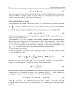
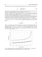
the following properties (see Fig. 1): (i) the interior of V is divided by N−1 surfaces S
j
(j=2, ,N) into N annuli-like regions (layers) V
j
(j=1, ,N), (ii) S
j
are C
2
surfaces with S
j
containing S
j+1
and dist(S
j
, S
j+1

) > 0, (iii) the layers V
j
(j=1, ,N−1), are homogeneous
isotropic media specified by real wavenumbers k
j
and mass densities ρ
j
, (iv) the scatterer’s
core V
N
(containing the origin of coordinates) is penetrable specified by real wavenumber
k
N
and mass density ρ
N
or impenetrable being soft, hard or resistive. The exterior V
0
of the
scatterer V is a homogeneous isotropic medium with real constants k
0
and ρ
0
. In any layer V
j
the Green’s second theorem is valid by considering the surfaces S
j
as oriented by the outward
normal unit vector
ˆ
n.

The layered scatterer V is excited by a time harmonic (exp(−iωt) time dependence) spherical
acoustic wave, generated by a point source with position vector r
q
in the layer V
q
(q=0, ,N).
Applying Sommerfeld’s method (see for example (20), (21), (22)), the primary spherical field
u
pr
r
q
, radiated by this point-source, is expressed by
u
pr
r
q
(r) = r
q
exp(−ik
q
r
q
)
exp(ik
q
|r −r
q
|)
|r −r
q

|
, r ∈ R
3
\{r
q
}, (1)
where r
q
=|r
q
|. We have followed the normalization introduced in (5), namely considered that
the primary field reduces to a plane wave with direction of propagation that of the unit vector
−ˆr
q
, when the point source recedes to infinity, i.e.
lim
r
q
→∞
u
pr
r
q
(r) = exp(−ik
q
ˆr
q
·r). (2)
The scatterer V perturbs the primary field u
pr

r
q
, generating secondary fields in every layer
V
j
. The respective secondary fields in V
j
(j = q) and V
q
are denoted by u
j
r
q
and u
sec
r
q
. By
Sommerfeld’s method, the total field u
q
r
q
in V
q
is defined as the superposition of the primary
and the secondary field
u
q
r
q

(r) = u
pr
r
q
(r) + u
sec
r
q
(r), r ∈ V
q
\{r
q
}. (3)
Moreover, the total field in V
j
(j = q) coincides with the secondary field u
j
r
q
.
The total field u
j
r
q
in layer V
j
satisfies the Helmholtz equation
∆u
j
r

q
(r) + k
2
j
u
j
r
q
(r) = 0, (4)
for r ∈ V
j
if j = q and r ∈ V
q
\{r
q
} if j = q.
On the surfaces S
q
and S
q+1
the following transmission boundary conditions are required
u
q−1
r
q
(r) − u
sec
r
q
(r) = u

pr
r
q
(r), r ∈ S
q
(5)
1
ρ
q−1
∂u
q−1
r
q
(r)
∂n
−
1
ρ
q
∂u
sec
r
q
(r)
∂n
=
1
ρ
q
∂u

pr
r
q
(r)
∂n
, r ∈ S
q
295
Inverse Scattering in the Low-Frequency Region by Using Acoustic Point Sources
4 Acoustic Wave book 1
6
M
#
6
Q
#
]
\
3
0
\
V V

\
9
T
9
Q
6


#
6
T
6
T
6
M
#
6
1
#
]
\
3
0
\
V V

\
9
T
9
1
[
U
T
Fig. 1. Typical cross-section of the layered scatterer V.
u
q+1
r

q
(r) − u
sec
r
q
(r) = u
pr
r
q
(r), r ∈ S
q+1
(6)
1
ρ
q+1
∂u
q+1
r
q
(r)
∂n
−
1
ρ
q
∂u
sec
r
q
(r)

∂n
=
1
ρ
q
∂u
pr
r
q
(r)
∂n
, r ∈ S
q+1
Furthermore, on the surfaces S
j
(j = q, q + 1, N) the total fields must satisfy the transmission
conditions
u
j−1
r
q
(r) − u
j
r
q
(r) = 0, r ∈ S
j
(7)
1
ρ

j−1
∂u
j−1
r
q
(r)
∂n
−
1
ρ
j
∂u
j
r
q
(r)
∂n
= 0, r ∈ S
j
For a penetrable core (7) hold also for j=N. On the other hand, for a soft, hard and resistive
core the total field on S
N
must satisfy respectively
the Dirichlet
u
N−1
r
q
(r) = 0, r ∈ S
N

(8)
296
Waves in Fluids and Solids
V V
V V
Inverse Scattering in the Low-Frequency Region by Using Acoustic Point Sources 5
the Neumann
∂u
N−1
r
q
(r)
∂n
= 0, r ∈ S
N
(9)
and the Robin boundary condition
∂u
N−1
r
q
(r)
∂n
+ ik
N−1
λu
N−1
r
q
(r) = 0, r ∈ S

N
(λ ∈ R). (10)
The first of Eqs. (5), (6), (7) and Eq. (8) represent the continuity of the fluid’s pressure, while
the second of Eqs. (5), (6), (7) and Eq. (9) represent the continuity of the normal components of
the wave’s speed. Detailed discussion on the physical parameters of acoustic wave scattering
problems is contained in (4).
Since scattering problems always involve an unbounded domain, a radiation condition for the
total field in V
0
must be imposed. Thus, u
0
r
q
must satisfy the Sommerfeld radiation condition
(10)
∂u
0
r
q
(r)
∂n
−ik
0
u
0
r
q
(r) = o(r
−1
), r → ∞ (11)

uniformly for all directions
ˆ
r of R
3
, i.e.
ˆ
r ∈ S
2
= {x ∈ R
3
, |x| = 1}. Note that a primary
spherical acoustic wave defined by (1) satisfies the Sommerfeld radiation condition (11), which
clearly is not satisfied by an incident plane acoustic wave.
Besides, the secondary u
sec
r
0
and the total field u
0
r
q
in V
0
have the asymptotic expressions
u
sec
r
0
(r) = g
r

0
(ˆr)h
0
(k
0
r) + O(r
−2
), r → ∞ (12)
u
0
r
q
(r) = g
r
q
(ˆr)h
0
(k
0
r) + O(r
−2
), r → ∞ (q > 0) (13)
where h
0
(x)=exp(ix)/(ix) is the zero-th order spherical Hankel function of the first kind. The
function g
r
q
is the q-excitation far-field pattern and describes the response of the scatterer in the
direction of observation ˆr of the far-field, due to the excitation by the particular primary field

u
pr
r
q
in layer V
q
.
Moreover, we define the q-excitation differential (or bistatic radar) cross-section
σ
r
q
(
ˆ
r) =
4π
k
2
0
|g
r
q
(
ˆ
r)|
2
, (14)
which specifies the amount of the field’s power radiated in the direction
ˆ
r of the far field. Also,
we define the q-excitation total cross-section

σ
r
q
=
1
k
2
0

S
2
|g
r
q
(
ˆ
r)|
2
ds(
ˆ
r), (15)
representing the average of the amount of the field’s power radiated in the far-field over all
directions, due to the excitation of the layered scatterer V by a point-source located in layer
V
q
. Thus, σ
r
q
is the average of σ
r

q
(
ˆ
r) over all directions. We note that the definition (15) of σ
r
q
extends that of the scattering cross-section (see (5) of (8) or (17) of (5)) due to a point-source at
r
0
∈ R
3
\V.
Finally, we define the absorption and the extinction cross-section
σ
a
r
q
=
ρ
0
ρ
N−1
k
0
Im



S
N

u
N−1
r
q
(r)
∂
u
N−1
r
q
(r)
∂n
ds(r)


, (16)
297
Inverse Scattering in the Low-Frequency Region by Using Acoustic Point Sources
6 Acoustic Wave book 1
σ
e
r
q
= σ
a
r
q
+ σ
r
q

. (17)
The former determines the amount of primary field power, absorbed by the core V
N
(since all
the other layers have been assumed lossless) and the latter the total power that the scatterer
extracts from the primary field either by radiation in V
0
or by absorption. Clearly, σ
a
r
q
= 0 for
a soft, hard, or penetrable lossless core, and σ
a
r
q
≥ 0 for a resistive core.
We note that scattering theorems for the interior acoustic excitation of a layered obstacle,
subject to various boundary conditions, have been treated in (23) and (24).
3. Layered sphere: direct scattering problems
The solution of the direct scattering problem for the layered scatterer of Fig. 1 cannot
be obtained analytically and thus generally requires the use of numerical methods; for an
overview of such methods treating inhomogeneous and partially homogeneous scatterers
see (25). However, for spherical surfaces S
j
, the boundary value problem can be solved
analytically and the exact Green’s function can be obtained in the form of special functions
series. To this end, we focus hereafter to the case of the scatterer V being a layered sphere.
By adjusting the general description of Section 2, the spherical scatterer V has radius a
1

and surface S
1
, while the interior of V is divided by N−1 concentric spherical surfaces S
j
,
defined by r = a
j
(j=2, ,N) into N layers V
j
(j=1, ,N) (see Fig. 2). The layers V
j
, defined
by a
j+1
≤ r ≤ a
j
(j=1, ,N−1), are filled with homogeneous materials specified by real
wavenumbers k
j
and mass densities ρ
j
.
3.1 Exact acoustic Green’s function
A classic scattering problem deals with the effects that a discontinuity of the medium of
propagation has upon a known incident wave and that takes care of the case where the
excitation is located outside the scatterer. When the source of illumination is located inside
the scatterer and we are looking at the field outside it, then we have a radiation and not
a scattering problem. The investigation of spherical wave scattering problems by layered
spherical scatterers is usually based on the implementation of T-matrix (22) combined with
Sommerfeld’s methods (20), (21). The T-matrix method handles the effect of the sphere’s

layers and the Sommerfeld’s method handles the singularity of the point-source and unifies
the cases of interior and exterior excitation. The combination of these two methods leads
to certain algorithms for the development of exact expressions for the fields in every layer.
Here, we impose an appropriate combined Sommerfeld T-matrix method for the computation
of the exact acoustic Green’s function of a layered sphere. More precisely, the primary and
secondary acoustic fields in every layer are expressed with respect to the basis of the spherical
wave functions. The unknown coefficients in the secondary fields expansions are determined
analytically by applying a T-matrix method.
We select the spherical coordinate system (r,θ,φ) with the origin O at the centre of V, so that
the point-source is at r=r
q
, θ=0. The primary spherical field (1) is then expressed as (19)
u
pr
r
q
(r, θ) =
1
h
0
(k
q
r
q
)

∑
∞
n=0
(2n + 1)j

n
(k
q
r
q
)h
n
(k
q
r)P
n
(cos θ), r > r
q
∑
∞
n=0
(2n + 1)h
n
(k
q
r
q
)j
n
(k
q
r)P
n
(cos θ), r < r
q

where j
n
and h
n
are the n-th order spherical Bessel and Hankel function of the first kind and
P
n
is a Legendre polynomial.
298
Waves in Fluids and Solids
Inverse Scattering in the Low-Frequency Region by Using Acoustic Point Sources 7
]
\
[
9

9
1í
9
1
9
T
D
T
D

D

D
1í

D
1
6
1
6
1í
6
T
6

6

U
T







6
T
D
T
3
0
\
V V

\






Fig. 2. Geometry of the layered spherical scatterer.
The secondary field u
j
r
q
in V
j
(j=1, ,N−1) is expanded as
u
j
r
q
(r, θ) =
∞
∑
n=0
(2n + 1)
h
n
(k
q
r
q

)
h
0
(k
q
r
q
)

α
j
q,n
j
n
(k
j
r) + β
j
q,n
h
n
(k
j
r)

P
n
(cos θ), (18)
where α
j

q,n
and β
j
q,n
under determination coefficients. The secondary field in V
0
has the
expansion (18) with j=0 and α
0
q,n
= 0, valid for r ≥ a
1
, in order that the radiation condition (11)
is satisfied. On the other hand, since zero belongs to V
N
, the secondary field in a penetrable
core V
N
has the expansion (18) with j=N and β
N
q,n
=0, valid for 0 ≤ r ≤ a
N
.
By imposing the boundary conditions (7) on the spherical surfaces S
j
, we obtain the
transformations

α

j
q,n
β
j
q,n

= T
j
n

α
j−1
q,n
β
j−1
q,n

(19)
The 2×2 transition matrix T
j
n
from V
j−1
to V
j
, which is independent of the point-source’s
location, is given by
T
j
n

= −ix
2
j

h
′
n
(x
j
)j
n
(y
j
) − w
j
h
n
(x
j
)j
′
n
(y
j
) h
′
n
(x
j
)h

n
(y
j
) − w
j
h
n
(x
j
)h
′
n
(y
j
)
w
j
j
n
(x
j
)j
′
n
(y
j
) − j
′
n
(x

j
)j
n
(y
j
) w
j
j
n
(x
j
)h
′
n
(y
j
) − j
′
n
(x
j
)h
n
(y
j
)

,
where x
j

= k
j
a
j
, y
j
= k
j−1
a
j
, w
j
= (k
j−1
ρ
j
)/(k
j
ρ
j−1
).
299
Inverse Scattering in the Low-Frequency Region by Using Acoustic Point Sources
8 Acoustic Wave book 1
Since α
0
q,n
=0, successive application of (19) for j=1, ,q leads to

α

q
q,n
β
q
q,n
+
j
n
(k
q
r
q
)
h
n
(k
q
r
q
)

= T
+
q,n

0
β
0
q,n


(20)
where
T
+
q,n
= T
q
n
T
2
n
T
1
n
. (21)
In a similar way successive application of (19) for j=q+1, ,N −1 gives

α
N−1
q,n
β
N−1
q,n

= T
−
q,n

α
q

q,n
+ 1
β
q
q,n

(22)
where
T
−
q,n
= T
N−1
n
T
q+2
n
T
q+1
n
. (23)
The superscripts + in (20) and − in (22) indicate approach of the layer V
q
, containing the
point-source, from the layers above and below respectively.
Then, the coefficient of the secondary field in layer V
0
is determined by combining (20) and
(22) and imposing the respective boundary condition on the surface of the core V
N

, yielding
β
0
q,n
=

j
n
(k
q
r
q
)

f
n
(k
N−1
a
N
)

T
−
q,n

12
+ g
n
(k

N−1
a
N
)

T
−
q,n

22

−h
n
(k
q
r
q
)

f
n
(k
N−1
a
N
)

T
−
q,n


11
+ g
n
(k
N−1
a
N
)

T
−
q,n

21


· (24)

h
n
(k
q
r
q
)

f
n
(k

N−1
a
N
)

T
−
q,n
T
+
q,n

12
+ g
n
(k
N−1
a
N
)

T
−
q,n
T
+
q,n

22



−1
where
f
n
= j
n
, j
′
n
, and j
′
n
+ iλj
n
g
n
= h
n
, h
′
n
, and h
′
n
+ iλh
n
for a soft, hard and resistive core respectively, while for a penetrable core we obtain
β
0

q,n
=
j
n
(k
q
r
q
)

T
N
n
T
−
q,n

22
− h
n
(k
q
r
q
)

T
N
n
T

−
q,n

21
h
n
(k
q
r
q
)

T
N
n
T
−
q,n
T
+
q,n

22
. (25)
Moreover, by using the above explicit expression for β
0
q,n
we see that the coefficients α
j
q,n

and
β
j
q,n
, describing the field in layer V
j
(j=1,2, ,N), are determined by successive application of
the transformations (19).
By using the above method we recover (for q=0 and N=1) classic results of the literature,
concerning the scattered field for the exterior point-source excitation of a homogeneous sphere
(see for example (10.5) and (10.70) of (2) for a soft and a hard sphere).
A basic advantage of the proposed method is that the coefficients β
0,N+1
q,n
of the secondary field
in the exterior V
0
of an N+1-layered spherical scatterer with penetrable core may be obtained
directly by means of the coefficients β
0,N
q,n
of the corresponding N-layered scatterer by means
of an efficient recursive algorithm (19).
300
Waves in Fluids and Solids
Inverse Scattering in the Low-Frequency Region by Using Acoustic Point Sources 9
Furthermore, for any type of core the q-excitation far field pattern is given by
g
r
q

(θ) =
1
h
0
(k
q
r
q
)
∞
∑
n=0
(2n + 1)(−i)
n
β
0
q,n
h
n
(k
q
r
q
)P
n
(cos θ). (26)
This expression follows by (12), (13) and (18) for j=0 and by taking into account the asymptotic
expression h
n
(z) ∼ (−i)

n
h
0
(z), z → ∞. By (14) and (26) we get the q-excitation bistatic radar
cross-section
σ
r
q
(θ) = 4πr
2
q
k
2
q
k
2
0




∞
∑
n=0
(2n + 1)(−i)
n
β
0
q,n
h

n
(k
q
r
q
)P
n
(cos θ)




2
. (27)
Now, by combining (15) with (26) and using the Legendre functions orthogonality properties
((27), (7.122) and (7.123)), we get the expression of the q-excitation total cross-section
σ
r
q
= 4πr
2
q
k
2
q
k
2
0
∞
∑

n=0
(2n + 1)|β
0
q,n
h
n
(k
q
r
q
)|
2
. (28)
Next, we will give some numerical results concerning the far-field interactions between the
point-source and the layered sphere. In particular, we will make a comparative far-field
investigation of spherical and plane wave scattering, which provides certain numerical criteria
on how far the point-source should be placed from the sphere in order to obtain the same
results with plane wave incidence. This knowledge is important for the implementation of
the far-field inverse scattering algorithms described in Section 4.1 below.
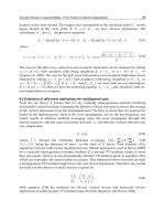
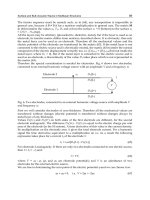
Figs. 3a, 3b, and 3c depict the normalized 0-excitation total cross-section σ
r
0
/2πa
2
1
as a
function of k
0
a
1

for a soft, hard, and penetrable sphere for three different point-source
locations, as well as for plane wave incidence. The cross-sections for spherical wave scattering
are computed by means of (28). On the other hand, by using (28) and taking into account that
h
n
(k
0
r
0
) ∼ (−i)
n
h
0
(k
0
r
0
), r
0
→ ∞, we obtain
σ =
4π
k
2
0
∞
∑
n=0
(2n + 1)|β
0

0,n
|
2
,
which is utilized for the cross-sections computations due to plane wave scattering.
The cross-section curves reduce to those due to plane wave incidence for large enough
distances between the point-source and the scatterer. The critical location of the point-source
where the results are almost the same with those of plane wave incidence depends on the
type of boundary condition on the sphere’s surface. In particular, for point-source locations
with distances of more than 8, 5, and 8 radii a
1
from the center of a soft, hard, and penetrable
sphere, the results are the same with the ones corresponding to plane wave incidence. We
note that those cross-section curves of Figs. 3a and 3b referring to plane wave incidence on a
soft and hard sphere coincide with those of Figs. 10.5 and 10.12 of (2).
The 0-excitation total cross-section σ
r
0
increases as the point-source approaches the sphere
(r
0
→a
1
) and hence the effect of the spherical wave on the sphere’s far-field characteristics
increases compared with that of the plane wave. Moreover, σ
r
0
of a penetrable sphere as a
function of k
0

a
1
is very oscillatory (see Fig. 3c). These oscillations are due to the penetrable
material of the sphere and hence do not appear in the cases of soft or hard sphere. Besides,
Fig. 3c indicates that σ
r
0
of a penetrable sphere is oscillatory also as k
0
a
1
→∞, while for the
other cases converges rapidly.
301
Inverse Scattering in the Low-Frequency Region by Using Acoustic Point Sources
10 Acoustic Wave book 1
0 1 2 3 4 5 6 7 8 9 10
1.2
1.3
1.4
1.5
1.6
1.7
1.8
1.9
2
k
0
a
1

σ
r
0
/2π a
1
2
soft sphere
r
0
=1.1a
1
r
0
=1.5a
1
r
0
=8a
1
plane wave
0 1 2 3 4 5 6 7 8 9 10
0
0.1
0.2
0.3
0.4
0.5
0.6
0.7
0.8

0.9
1
k
0
a
1
σ
r
0
/2π a
1
2
r
0
=1.1a
1
r
0
=1.5a
1
r
0
=5a
1
plane wave
hard sphere
0 1 2 3 4 5 6 7 8 9 10
0
1
2

3
4
5
6
7
k
0
a
1
σ
r
0
/2π a
1
2
r
0
=1.1a
1
r
0
=1.5a
1
r
0
=8a
1
plane wave
penetrable sphere
Fig. 3. Normalized 0-excitation total cross-section σ

r
0
/2πa
2
1
as a function of k
0
a
1
for (a) a soft,
(b) a hard, and (c) a penetrable (η
1
=3, ̺
1
=2) sphere for various point-source locations and
plane wave incidence
302
Waves in Fluids and Solids
Inverse Scattering in the Low-Frequency Region by Using Acoustic Point Sources 11
3.2 Far-field results for a small layered sphere
All formulae derived up to now are exact. Now, we make the so-called low-frequency
assumption k
0
a
1
≪ 1 for the case of 3-layered sphere with any type of core, that is assume
that the radius a
1
of the sphere is much smaller than the wavelength of the primary field. In
order to establish the low-frequency results, we use the following dimensionless parameters

ξ
1
= a
1
/a
2
, ξ
2
= a
2
/a
3
, ̺
i
= ρ
i
/ρ
0
, η
i
= k
i
/k
0
, κ = ik
0
a
1
,
where ξ

1
and ξ
2
represent the thicknesses of layers V
1
and V
2
and ̺
i
and η
i
the relative with
respect to free space mass densities and refractive indices of layers V
i
(i=1,2,3).
The following two cases are analyzed: (i) exterior excitation by a point-source located at
(0,0,r
0
) with r
0
> a
1
, lying in the exterior V
0
of the sphere, and (ii) interior excitation by a
point-source located at (0,0,r
1
) with a
2
< r

1
< a
1
, lying in layer V
1
of the 3-layered sphere. We
define also
τ
i
= a
1
/r
i
, d = r
1
/a
2
(i = 0, 1),
where τ
0
represents the distance of the exterior point-source from the sphere’s surface and τ
1
and d the distances of the interior point-source from the boundaries of layer V
1
.
Now, we distinguish the following cases according to the types of the core V
3
.
(a) V
3

is soft
By using the asymptotic expressions of the spherical Bessel and Hankel functions for small
arguments ((26), (10.1.4), (10.1.5)), from (24) we obtain
β
0
q,0
= S
1
q,0
κ + S
2
q,0
κ
2
+ S
3
q,0
κ
3
+ O(κ
4
), κ → 0 (q = 0, 1) (29)
β
0
0,n
∼
(k
0
a
1

)
2n+1
i(2n + 1)c
2
n
S
0,n
, β
0
1,n
∼
η
n
1
(k
0
a
1
)
2n+1
ic
2
n
S
1,n
, k
0
a
1
→ 0 (n ≥ 1) (30)

where
c
n
= 1 ·3 ·5 ···(2n −1), c
0
= 1,
and the quantities S
j
q,0
(j=1,2,3) and S
q,n
depend on the parameters ξ
1
, ξ
2
, ̺
1
, ̺
2
, d and are
given in the Appendix of (19).
In order to calculate the q-excitation far-field patterns with an error of order κ
4
, the coefficients
β
0
q,0
, β
0
q,1

and β
0
q,2
are sufficient. For κ → 0, (26) gives the approximation of the q-excitation
far-field patterns
g
r
0
(θ) = S
1
0,0
κ +

S
2
0,0
+ τ
0
S
0,1
P
1
(cos θ)

κ
2
+

S
3

0,0
−S
0,1
P
1
(cos θ) −
τ
2
0
3
S
0,2
P
2
(cos θ)

κ
3
+ O(κ
4
) (31)
g
r
1
(θ) = S
1
1,0
κ +

S

2
1,0
+ 3τ
1
S
1,1
P
1
(cos θ)

κ
2
+

S
3
1,0
−3η
1
S
1,1
P
1
(cos θ) −
5
3
τ
2
1
S

1,2
P
2
(cos θ)

κ
3
+ O(κ
4
) (32)
303
Inverse Scattering in the Low-Frequency Region by Using Acoustic Point Sources
12 Acoustic Wave book 1
By (28) the calculation of the q-excitation total cross-sections to the same accuracy requires
only β
0
q,0
and β
0
q,1
, giving for κ → 0 the approximations
σ
r
0
= 4πa
2
1

(S
1

0,0
)
2
+ k
2
0
a
2
1

(S
2
0,0
)
2
−2S
1
0,0
S
3
0,0
+
τ
2
0
3
(S
0,1
)
2


+ O(κ
4
) (33)
σ
r
1
= 4πa
2
1

(S
1
1,0
)
2
+ k
2
0
a
2
1

(S
2
1,0
)
2
−2S
1

1,0
S
3
1,0
+ 3τ
2
1
(S
1,1
)
2

+ O(κ
4
). (34)
(b) V
3
is hard
The respective results are as follows
β
0
q,0
= H
1
q,0
κ + H
2
q,0
κ
2

+ H
3
q,0
κ
3
+ O(κ
5
), κ → 0 (q = 0, 1) (35)
β
0
0,n
∼
n
n + 1
(k
0
a
1
)
2n+1
i(2n + 1)c
2
n
H
0,n
, β
0
1,n
∼
η

n
1
(k
0
a
1
)
2n+1
i(n + 1)c
2
n
H
1,n
, k
0
a
1
→ 0 (n ≥ 1), (36)
where the quantities H
j
q,0
(j=1,2,3) and H
q,n
, depending on ξ
1
, ξ
2
, ̺
1
, ̺

2
, d, are given in the
Appendix of (19).
Now, by using (26) and (28) we obtain the low-frequency expansions of the q-excitation
far-field patterns and total cross-sections as κ → 0
g
r
0
(θ) =
τ
0
2
H
0,1
P
1
(cos θ)κ
2
+

H
3
0,0
−
H
0,1
2
P
1
(cos θ) −

2τ
2
0
9
H
0,2
P
2
(cos θ)

κ
3
+ O(κ
4
), (37)
g
r
1
(θ) = H
1
1,0
κ +

H
2
1,0
+
3
2
τ

1
H
1,1
P
1
(cos θ)

κ
2
+

H
3
1,0
−
3
2
η
1
H
1,1
P
1
(cos θ) +
5
9
τ
2
1
H

1,2
P
2
(cos θ)

κ
3
+ O(κ
4
), (38)
σ
r
0
= πa
2
1
τ
2
0
3
(H
0,1
)
2
(k
0
a
1
)
2

+ O(κ
4
) (39)
σ
r
1
= 4πa
2
1

(H
1
1,0
)
2
+ k
2
0
a
2
1

(H
2
1,0
)
2
−2H
1
1,0

H
3
1,0
+
3
4
τ
2
1
(H
1,1
)
2

+ O(κ
4
). (40)
(c) V
3
is penetrable
From (25) we have
β
0
1,0
= P
1
1,0
κ + P
2
1,0

κ
2
+ P
3
1,0
κ
3
+ O(κ
4
), κ → 0 (41)
β
0
0,n
∼
ink
2n+1
0
a
2n+1
1
c
2
n
(2n + 1)
P
0,n
, β
0
1,n
∼

iη
n
1
(k
0
a
1
)
2n+1
c
2
n
P
1,n
k
0
a
1
→ 0 (n ≥ 1), (42)
where the quantities P
j
1,0
(j=1,2,3) and P
q,n
depend on the parameters ξ
1
, ξ
2
, ̺
1

, ̺
2
, ̺
3
, d and
are given in the Appendix of (19).
304
Waves in Fluids and Solids
Inverse Scattering in the Low-Frequency Region by Using Acoustic Point Sources 13
From (26) we obtain for κ → 0 the approximation of the q-excitation far-field patterns and
total cross-sections
g
r
0
(θ) = κ
2
(κ − τ
0
)P
0,1
P
1
(cos θ) +
2
3
κ
3
τ
2
0

P
0,2
P
2
(cos θ) + O(κ
4
), (43)
g
r
1
(θ) = P
1
1,0
κ +

P
2
1,0
−3τ
1
P
1,1
P
1
(cos θ)

κ
2
+


P
3
1,0
+ 3η
1
P
1,1
P
1
(cos θ) +
5
3
τ
2
1
P
1,2
P
2
(cos θ)

κ
3
+ O(κ
4
), (44)
σ
r
0
= −4πa

2
1
κ
2
τ
2
0
3
(P
0,1
)
2
+ O(κ
4
) (45)
σ
r
1
= 4πa
2
1

(P
1
1,0
)
2
+ k
2
0

a
2
1

(P
2
1,0
)
2
−2P
1
1,0
P
3
1,0
+ 3τ
2
1
(P
1,1
)
2

+ O(κ
4
). (46)
For a small layered sphere with a resistive core the corresponding far-field results are given in
(19).
We note that: (i) for a soft core the leading order terms of the far-field patterns g
r

q
and total
cross-sections σ
r
q
are of order κ
1
and κ
0
independently of q, (ii) for a hard, resistive, and
penetrable core the leading order terms of g
r
q
and σ
r
q
are of order κ
2
for q=0 and κ
1
and κ
0
for
q=1. Thus, the interaction characteristics of spheres with hard, resistive, and penetrable cores
change drastically for point-sources embedded inside the sphere. This last fact is exploited
appropriately in certain inverse scattering algorithms, described below.
Now, concerning certain reductions of the above derived low-frequency far-field results,
we note that the point-source incident field (1) for r
0
→∞ (τ

0
→0) reduces to the plane
wave (2). Thus, the preceding far-field results for τ
0
→0 reduce to the respective ones,
corresponding to the plane wave incidence on a 3-layered sphere with soft, hard, and
penetrable core V
3
respectively. We remark that the leading term approximations of the
0-excitation cross-sections (39) and (45) for a hard and penetrable core are zero for τ
0
= 0.
Hence the interaction of a layered sphere with hard and penetrable core with an incident
low-frequency field is weaker when the incident field is a plane wave than when it is a
spherical wave.
Moreover, concerning the spherical wave excitation of a 2-layered sphere with various types
of cores, the far-field results are derived by the respective above ones for ξ
2
= 1, ̺
2
= ̺
1
,
̺
3
= ̺
2
, and η
2
= η

1
. On the other hand, the derived low-frequency far-field results recover
(for ξ
1
= ξ
2
= 1, ̺
1
= ̺
2
= 1, η
1
= η
2
= 1) several results of the literature, concerning
the exterior spherical wave excitation of 1-layered (homogeneous) small spheres, subject to
various boundary conditions; for more details see (19). Besides, by letting also τ
0
→ 0 they
recover classic low-frequency far-field results for plane wave incidence; see (10.28) of (2) and
(7.33), (7.35), (7.42), (7.53), (7.55) and (7.66) of (4).
Importantly, the convergence of the low-frequency total cross-section to the exact one plays a
significant role in the inverse scattering algorithms described in Section 4 below. To this end,
here we will investigate numerically the convergence of the low-frequency q-excitation total
cross-section to the exact one for a 3-layered sphere with various types of cores. Figs. 4 and
5 depict the exact and low-frequency normalized q-excitation total cross-section σ
r
q
/2πa
2

1
as a
function of k
0
a
1
for a 3-layered sphere with soft and hard core. The exact total cross-sections
are computed by means of (28), while the low-frequency ones by (33), (34), (39), and (40).
For small k
0
a
1
the convergence of the low-frequency to the exact total cross-section is excellent
for all types of cores with weak and strong coatings subject to both interior and exterior
305
Inverse Scattering in the Low-Frequency Region by Using Acoustic Point Sources
14 Acoustic Wave book 1
0 0.05 0.1 0.15 0.2 0.25 0.3
0.4
0.5
0.6
0.7
0.8
0.9
1
1.1
k
0
a
1

σ
r
q
/2π a
1
2
low−frequency, q=0
exact, q=0
low−frequency, q=1
exact, q=1
soft core V
3
with "weak" coating
0 0.05 0.1 0.15 0.2 0.25 0.3
0
0.1
0.2
0.3
0.4
0.5
0.6
0.7
k
0
a
1
σ
r
q
/2π a

1
2
low−frequency, q=0
exact, q=0
low−frequency, q=1
exact, q=1
soft core V
3
with "strong" coating
Fig. 4. Exact and low-frequency q-excitation total cross-section σ
r
q
/2πa
2
1
as a function of k
0
a
1
for a 3-layered sphere (a
2
=0.5a
1
, a
3
=0.25a
1
) with soft core with (a) weak (η
1
=1.4, η

2
=1.6,
̺
1
=1.2, ̺
2
=1.4), and (b) strong (η
1
=2, η
2
=3, ̺
1
=3, ̺
2
=2) coating. The two point-source
locations are r
0
= 1.1a
1
and r
1
= 1.1a
2
.
306
Waves in Fluids and Solids
Inverse Scattering in the Low-Frequency Region by Using Acoustic Point Sources 15
0 0.05 0.1 0.15 0.2 0.25 0.3
0
1

2
3
4
5
6
7
x 10
−3
k
0
a
1
σ
r
0
/2π a
1
2
low−frequency, q=0
exact, q=0
hard core V
3
with "weak" coating
0 0.05 0.1 0.15 0.2 0.25 0.3
2.62
2.64
2.66
2.68
2.7
2.72

2.74
2.76
2.78
2.8
k
0
a
1
σ
r
1
/2π a
1
2
low−frequency, q=1
exact, q=1
hard core V
3
with "weak" coating
0 0.05 0.1 0.15 0.2 0.25 0.3
0
0.2
0.4
0.6
0.8
1
1.2
1.4
k
0

a
1
σ
r
q
/2π a
1
2
low−frequency, q=0
exact, q=0
low−frequency, q=1
exact, q=1
hard core V
3
with "strong" coating
Fig. 5. Exact and low-frequency q-excitation total cross-section σ
r
q
/2πa
2
1
as a function of k
0
a
1
for a 3-layered sphere with hard core with (a) and (b) weak, and (c) strong coating.
307
Inverse Scattering in the Low-Frequency Region by Using Acoustic Point Sources
16 Acoustic Wave book 1
excitation. However, even for k

0
a
1
lying outside the low-frequency region, good convergence
is also achieved.
In the low-frequency region, the 1-excitation total cross-sections are much larger than the
0-excitation ones. This is the reverse situation to that occurring outside the low-frequency
region, as discussed above, where the 0-excitation cross-section is larger that the 1-excitation.
So, interior and exterior excitations constitute control mechanisms of the far-field intensity,
depending on the desired application.
3.3 Near-field results for a small layered sphere
We consider a 2-layered sphere with soft core excited by an exterior source and still continue
to adopt the low-frequency assumption k
0
a
1
≪ 1, that is we assume that the outer radius
of the layered sphere, a
1
, is much smaller than the wavelength of the primary field. More
precisely, we suppose that k
0
a
1
, k
0
r
0
, k
1

a
2
and k
1
r
q
are all small (the waves are long compared
to all geometrical lengths) whereas k
1
/k
0
and ρ
1
/ρ
0
are not assumed to be small. We define
and use the following dimensionless parameters
ξ = a
1
/a
2
, ̺ = ρ
1
/ρ
0
, η = k
1
/k
0
, κ = k

0
a
1
, τ
0
= a
1
/r
0
, d
1
= r
1
/a
2
= ξ/τ
1
. (47)
We use the asymptotic expressions of the spherical Bessel and Hankel functions for small
arguments ((26), (10.1.4), (10.1.5)) to obtain the approximations of the elements of the
transition matrix (19), as κ → 0, by means of which we derive approximations for the field
coefficients α
j
0,n
and β
j
0,n
. Then we estimate the secondary field at the source point, using
u
sec

r
0
(r
0
, 0) = h
0
(k
0
r
0
)
∞
∑
n=0
(2n + 1)β
0
0,n
[H
n
(k
0
r
0
)]
2
, (48)
where
H
n
(w) = h

n
(w)/h
0
(w).
Moreover, from (30), we get
β
0
0,n
∼
κ
2n+1
i(2n + 1)c
2
n
S
0,n
(ξ, ̺), κ → 0, (49)
where
S
0,n
(ξ, ̺) =
B
n
(ξ) + ̺ nA
n
(ξ)
∆
n
(ξ, ̺)
, ∆

n
(ξ, ̺) = B
n
(ξ) −̺ (n + 1)A
n
(ξ), (50)
A
n
(x) = 1 − x
2n+1
, B
n
(x) = n(x
2n+1
+ 1) + 1.
Now, since
H
n
(w) ∼ c
n
w
−n
as w → 0,
the small-κ approximation of (48) combined with (49) gives the following approximation of
the secondary field at the external point-source’s location
u
sec
r
0
(r

0
, 0) = −τ
0
exp(ik
0
r
0
)
∞
∑
n=0
S
n
(ξ, ̺) τ
2n
0
+ O(κ), (51)
308
Waves in Fluids and Solids
Inverse Scattering in the Low-Frequency Region by Using Acoustic Point Sources 17
as k
0
a → 0. Note that, contrary to the case of low-frequency far-field results (see for example
(19)), in the near-field every term of the infinite series contributes to the leading order O(1)
behaviour. Now, by means of (51) we get
|u
sec
r
0
(r

0
, 0)| =





τ
0
∞
∑
n=0
S
n
(ξ, ̺) τ
2n
0





+ O(κ
2
), (52)
as k
0
a → 0.
4. Layered sphere: inverse scattering problems
The low-frequency far- and near-field results, presented in Sections 3.2 and 3.3, are now

utilized for the development of far- and near-field inverse scattering algorithms for the
localization and reconstruction of the sphere’s characteristics.
4.1 Far-field inverse scattering problems
The low-frequency realm offers a better environment for inverse scattering, compared to
the exact yet complicated far-field series solutions (26) and (28), since the corresponding
low-frequency far-field patterns are much more tractable. In particular, we develop inverse
scattering algorithms for the determination of the geometrical and physical characteristics
of the 3-layered sphere and the point-source, based on low-frequency measurements of the
0- and 1- excitation total cross-section. Additionally, we emphasize that the embedding of
the point-source inside the scatterer offers additional essential information for the problem’s
characteristics, which cannot be given by a point-source outside the sphere.
4.1.1 Determination of the point-source’s location
We determine the location of the point-source for given geometrical and physical
characteristics of the sphere. This type of problem is expected to find applications in the
determination of the layer that the neuron currents radiate in investigations of the human
brain’s activity (15). An inverse scattering algorithm is established for the hard core case.
We use the 0- and 1- excitation total cross-sections (39) and (40) of a 3-layered sphere with
hard core. The decision on whether the point-source lies in the interior or the exterior of the
sphere is based on the following algorithmic criterion:
Measure the leading term (of order (k
0
a
1
)
0
) in the low-frequency expansion of the total
cross-section. If this measurement is zero, then from (39), the point-source is outside the
sphere. On the other hand, if this measurement is not zero then from (40) the point-source
is inside the sphere.
After determining the layer that the point-source is lying, we can also obtain its position r

q
(q=0,1). For exterior excitation, we compute the position r
0
from the measurement of the
leading order term of the 0-excitation total cross-section (39)
m
0
= πk
2
0
a
6
1
3r
2
0
(H
0,1
)
2
,
while for interior excitation, the measurement of the second order term of the 1-excitation total
cross-section (40)
309
Inverse Scattering in the Low-Frequency Region by Using Acoustic Point Sources
18 Acoustic Wave book 1
m
1
= 4πk
2

0
a
4
1

(H
2
1,0
)
2
−2H
1
1,0
H
3
1,0
+
3a
2
1
4r
2
1
(H
1,1
)
2

gives the position r
1

of the point-source.
4.1.2 Determination of the layers material parameters
We determine the mass densities of the sphere’s layers for given center’s coordinates and
layers radii of the sphere. Inverse scattering algorithms are established for a sphere with
penetrable core.
Consider two point-source locations (0,0,b
0
) and (0,0,b
1
) with known distances b
0
> a
1
and
a
2
< b
1
< a
1
from the layered sphere’s center (that is the first point-source lies in the
exterior and the second one in the interior of the scatterer). First, measure the leading order
low-frequency term m
0
of the 0-excitation total cross-section (45) for a point-source at (0,0,b
0
)
m
0
=

4πk
2
0
a
6
1
3b
2
0
(P
0,1
)
2
, (53)
and then the leading m
1
and the second order term m
2
of the 1-excitation total cross-section
(46) for a point-source at (0,0,b
1
)
m
1
= 4π
b
2
1
̺
2

1
, (54)
m
2
= 4πk
2
0
a
4
1

(P
2
1,0
)
2
−2P
1
1,0
P
3
1,0
+
3a
2
1
b
2
1
(P

1,1
)
2

. (55)
Eq. (54) provides the mass density ̺
1
of layer V
1
. Eqs. (53) and (55) constitute a 2 × 2
non-linear system, the solution of which provides the densities ̺
2
and ̺
3
of layers V
2
and
V
3
.
4.1.3 Determination of the sphere’s center and the layers radii
We determine the center’s coordinates and the layers radii of the 3-layered sphere for given
mass densities and refractive indices of the sphere’s layers. We establish the inverse scattering
algorithms for a sphere with soft core.
Choose a Cartesian coordinate system Oxyz and five point-source locations (0,0,0), (ℓ,0,0),
(0,ℓ,0), (0,0,ℓ), and (0,0,2ℓ) with unknown distances b
1
, b
2
, b

3
, b
4
and b
5
from the layered
sphere’s center. The parameter ℓ represents a chosen fixed length. First, measure the leading
order low-frequency term m
0
of the 0-excitation total cross-section (33) for a point-source
located at the origin
m
0
= 4πa
2
1
(S
1
0,0
)
2
(56)
Then, measure the second order low-frequency term m
j
of the 0-excitation total cross-section
(33) for each point-source location
m
j
= 4πk
2

0
a
4
1

(S
2
0,0
)
2
−2S
1
0,0
S
3
0,0
+
a
2
1
3b
2
j
(S
0,1
)
2

(j = 1, . . . , 5)
310

Waves in Fluids and Solids
Inverse Scattering in the Low-Frequency Region by Using Acoustic Point Sources 19
Measurability techniques permitting the isolation of the individual measurements m
0
and
m
j
from the total cross-section measurements as well as measurement sensitivity aspects are
discussed in (5).
Next, measure the second order cross-section term m
6
for a point-source far away from the
sphere (τ → 0) (namely for plane wave incidence)
m
6
= 4πk
2
0
a
4
1

(S
2
0,0
)
2
−2S
1
0,0

S
3
0,0

(57)
We define the dimensionless quantities
γ
j
=
ℓ

m
j
−m
6
=

3
4π
ℓ
k
0
a
2
1
S
0,1
b
j
a

1
. (58)
Now, we have seven equations with the eight unknowns a
1
, a
2
, a
3
, and b
j
. The 8-th equation
is derived by the law of cosines
b
2
5
= 2ℓ
2
+ 2b
2
4
−b
2
1
, (59)
and thus from (58) and (59) we get

b
j
ℓ


2
=
2γ
2
j
γ
2
5
−2γ
2
4
+ γ
2
1
,
which determine the distances b
j
. The intersection point of the four spheres centered at (0,0,0),
(ℓ,0,0), (0,ℓ,0), (0,0,ℓ) with determined radii b
1
, b
2
, b
3
, b
4
coincides with the center of the layered
spherical scatterer.
Finally, (56), (57), and (58) for j=1 constitute the 3×3 non-linear system
a

1
S
1
0,0
=

m
0
/4π
a
4
1

(S
2
0,0
)
2
−2S
1
0,0
S
3
0,0

= m
6
/(4πk
2
0

)
a
3
1
S
0,1
= (
√
3b
1
ℓ)/(
√
4πk
0
γ
1
),
which gives as solutions the layers radii a
1
, a
2
, and a
3
.
4.2 Near-field inverse scattering problems
The derived low-frequency near-field expansions in Section 3.3 are now utilized to establish
inverse scattering algorithms for the determination of the geometrical characteristics of the
piecewise homogeneous sphere. More precisely, the near-field inverse problem setting is as
follows: we know the sphere’s radius, a
1

, as well as the location of its center and we are
interested in estimating the core’s radius, a
2
. Note that for problems, where we need to
determine also the sphere’s radius and its center, appropriate modifications of the far-field
algorithms (to the present context of near-field measurements) presented in Section 6.1 of (19)
may be applied.
311
Inverse Scattering in the Low-Frequency Region by Using Acoustic Point Sources
20 Acoustic Wave book 1
Consider a 2-layered sphere with soft core. We suppose that the radius a
1
and the density
̺ are known and we will estimate the core’s radius a
2
by using a single measurement of
the near-field due to an exterior point-source. The corresponding near-field at the exterior
point-source’s location is given by (52). The series appearing in (52), namely
S (ξ, τ
0
, ̺) =
∞
∑
n=0
B
n
(ξ) + ̺ nA
n
(ξ)
B

n
(ξ) −̺ (n + 1)A
n
(ξ)
τ
2n
0
, (60)
may be expressed with the aid of Gauss hypergeometric functions, if we consider that the
relative mass density ̺ of the coating’s layer V
1
is close to 1. For this case, the series (60) has
the following properties
S (ξ, τ
0
, 1) =
1
ξ
∞
∑
n=0
1
2n + 1

τ
2
0
ξ
2


n
=
1
2τ
0
ln

ξ + τ
0
ξ − τ
0

, (61)
∂S
∂̺
(ξ, τ
0
, 1) =
1
ξ
2
∞
∑
n=0
nξ
2n+1
+ n + 1
2n + 1
(1 − ξ
2n+1

)

τ
2
0
ξ
4

n
=
1
ξ
2
F

2;
1
2
;
3
2
;
τ
2
0
ξ
4

−
τ

2
0
3
F

2;
3
2
;
5
2
; τ
2
0

−
1
2τ
0
ln

ξ + τ
0
ξ − τ
0

, (62)
where F ≡
2
F

1
is the Gauss hypergeometric function (26). Now, by considering the best linear
approximation around the fixed point ̺ = 1, from (60)-(62), we get
S (ξ, τ
0
, ̺) ≃ S (ξ, τ
0
, 1) +
∂S (ξ, τ
0
, 1)
∂̺
(̺ −1)
=
1
2τ
0
ln

ξ + τ
0
ξ − τ
0

(2 − ̺) −

1
ξ
2
F


2;
1
2
;
3
2
;
τ
2
0
ξ
4

−
τ
2
0
3
F

2;
3
2
;
5
2
; τ
2
0



(1 − ̺),
which in combination with (52) and (60) gives
|u
sec
r
0
(r
0
, 0)| =




2 −̺
2
ln

ξ + τ
0
ξ − τ
0

−

τ
0
ξ
2

F

2;
1
2
;
3
2
;
τ
2
0
ξ
4

−
τ
3
0
3
F

2;
3
2
;
5
2
; τ
2

0


(1 − ̺)




+ O(κ
2
). (63)
The radius a
2
of the core of the 2-layered sphere may now be determined by means of (63)
as follows. We measure the leading order term in the above low-frequency expansion of
|u
sec
r
0
(r
0
, 0)|, and we obtain a non-linear equation with respect ξ = a
1
/a
2
. Since, the radius
a
1
is known, the solution of this equation provides the core’s radius a
2

.
Similar near-field algorithms may be developed for a 2-layered sphere with hard, and
penetrable core.
5. Acknowledgement
The author’s work was supported by the State Scholarships Foundation, while he was a
post-doctoral research scholar.
312
Waves in Fluids and Solids
Inverse Scattering in the Low-Frequency Region by Using Acoustic Point Sources 21
6. References
[1] D. S. Jones, A new method for calculating scattering with particular reference to the
circular disc, Commun. Pure Appl. Math. 9 (1956) 713–746.
[2] J. J. Bowman, T. B. Senior, P. L. Uslenghi, Electromagnetic and Acoustic Scattering by Simple
Shapes, North Holland Publ. Co., 1969.
[3] D. S. Jones, Acoustic and Electromagnetic Waves, Oxford University Press, 1986.
[4] G. Dassios and R. Kleinman, Low Frequency Scattering, Clarendon Press, 2000.
[5] G. Dassios and G. Kamvyssas, Point source excitation in direct and inverse scattering:
the soft and the hard small sphere, IMA J. Appl. Math. 55 (1995) 67–84.
[6] G. Dassios and G. Kamvyssas, The impedance scattering problem for a point-source field.
The small resistive sphere, Quart. J. Mech. Appl. Math. 50 (1997) 321–332.
[7] G. Dassios, M. Hadjinicolaou and G. Kamvyssas, Direct and Inverse Scattering for Point
Source Fields. The Penetrable Small Sphere, Z. Angew. Math. Mech. 79 (1999) 303–316.
[8] C. Athanasiadis, P.A. Martin and I.G. Stratis, On spherical-wave scattering by a spherical
scatterer and related near-field inverse problems, IMA J. Appl. Math. 66 (2001) 539–549.
[9] C. J. S. Alves, and P. M. C. Ribeiro, Crack detection using spherical incident waves and
near-field measurements. Boundary Elements XXI, edited by C. A. Brebbia and H. Power
(WIT Press, Southampton, 1999) 355–364.
[10] D. Colton and R. Kress, Inverse acoustic and electromagnetic scattering theory,
Springer-Verlag, 1992.
[11] R. Potthast, Point-Sources and Multipoles in Inverse-Scattering Theory, Chapman and

Hall/CRC, 2001.
[12] J. Coyle, Locating the support of objects contained in a two-layered background medium
in two dimensions, Inverse Problems 16 (2000) 275–292.
[13] J. Kim and Y. Rahmat-Samii, Implanted Antennas Inside a Human Body: Simulations,
Designs, and Characterizations, IEEE Trans. Microwave Theory Tech. 52 (2004) 1934–1943.
[14] G. Dassios, A. S. Fokas and F. Kariotou, On the non-uniqueness of the inverse
magnetoencephalography problem, Inverse Problems 21 (2005) L1–L5.
[15] G. Dassios, On the hidden electromagnetic activity of the brain, in: Mathematical
Methods in Scattering Theory and Biomedical Engineering, Proceedings of the Seventh
International Workshop, World Scientific Publishing Co., 2006, pp. 297–303.
[16] K. Aki and P. G. Richards, Quantitative Seismology. Theory and Methods, Freeman, 1980.
[17] A. E. Yagle and B. C. Levy, Application of the Schur algorithm to the inverse problem for
a layered acoustic medium, J. Acoust. Soc. Am. 76 (1984) 301–308.
[18] A. Moroz, A recursive transfer-matrix solution for a dipole radiating inside and outside
a stratified sphere, Annals of Physics 315, (2005) 352–418.
[19] N. L. Tsitsas, and C. Athanasiadis, Point source excitation of a layered sphere: direct and
far-field inverse scattering problems, Quart. J. Mech. Appl. Math. 61, (2008) 549–580.
[20] A. Sommerfeld, Partial Differential Equations in Physics, Academic Press, 1949.
[21] J. A. Stratton, Electromagnetic Theory, McGraw-Hill, 1941.
[22] N. L. Tsitsas and C. Athanasiadis, On the scattering of spherical electromagnetic waves
by a layered sphere, Quart. J. Mech. Appl. Math. 59 (2006) 55–74.
[23] C. Athanasiadis, N. L. Tsitsas, Scattering theorems for acoustic excitation of a layered
obstacle by an interior point source, Stud. Appl. Math. 118 (2007), 397–418.
313
Inverse Scattering in the Low-Frequency Region by Using Acoustic Point Sources