Wind Energy Management Part 9 ppt
Bạn đang xem bản rút gọn của tài liệu. Xem và tải ngay bản đầy đủ của tài liệu tại đây (619.57 KB, 13 trang )
Superconducting Devices in Wind Farm
95
necessary, can be 5 - 10 for the size and weight optimization in both of the generator and the
gear system. The HTS generator used here is hybrid structured as widely suggested, i.e., its
rotor is made of HTS materials and the stator is conventional. Fig. 8 shows a schematic
diagram of the hybrid structured HTS generator. It consists of the HTS rotor, supported by
torsion transmitting tubes and sealed in a cryostat (often called Dewar in scientific reports),
and a conventional stator. For the convenience of connecting to the grid, the output voltage
of the system V is often selected as the common values used in the substations, for example,
10.5 kV and 35 kV in China. Similarly, the output of the system is usually in 3 phases, the
same as that in power grid. Thus, for designed capacity P, the output current I = 0.577P/V.
Fig. 7. The schematic diagram of a HTS generator system.
Fig. 8. The schematic diagram of the hybrid structured HTS generator. Labels in the figure:
1, Stator iron core; 2, Stator coil; 3, HTS rotor coil; 4, Rotor Dewar; 5, Torsion transmitting
tube; 6, Driving shaft; 7, Supporting tube; 8, Axial tube for cooling and current transition.
Wind Energy Management
96
However, adjusted by converter and transformer, the number of phases in the generator, as
well as the generator output voltage Vg and the stator phase current Ig are not necessarily
the same as those of the system, and can be optimized in generator electromagnetic design.
It is note worthy that adopting an AC – DC – AC converter between the generator and the
transformer, the output frequency of the generator fg can also be adjusted. It is usually very
low although the system output frequency f is commonly 50 or 60 Hz according to the grid
standards. This is advantageous because the number of magnetic poles in the rotor 2p,
which can be calculated by n = 60fg/p, decides the generator size and weight provided the
materials are the same. Reducing p is particularly beneficial in the “direct-driven” HTS
generators as the minimum bending diameters of commercial HTS wires are usually about
40 – 70 mm, which makes it difficult to wind magnetization coils smaller than NdFeB bulks,
and a rotor with many pairs of HTS coils would be large. In common, fg in a HTS generator
of several MW capacity can be 8 - 10 Hz to meet the speed requirement of the turbine, the
optimized coil size and weight, and electromagnetic design convenience at the same time.
Since DC resistance in HTS material is extremely small and only DC excitation current is
used for synchronous generator, the excitation power requirement of HTS generator is very
low. However, the field density in HTS coil is much larger than that in conventional ones,
the excitation current must be very stable, a stand alone power supply is then suggested for
exciting the HTS coils. Its input power can be in the altitude of 10 kW, while the output
current is 100 - 200 A, with very low fluctuations. Superconducting magnet power supply
made by the Bruker Corp. can be a good candidate for this. In emergency, this device can
even be activated by a set of batteries.
Besides the power supply, a cooling system is also necessary to the HTS generator. Depends
on the capacity and the rotor design, around 500 – 1000 W cooling power is needed. This can
be supplied by Stirling or G-M coolers, which give 200 - 500 W cooling power at ~ 77 K with
5 - 10 kW input power. At least two coolers are needed for one generator unit, an additional
one as backup is suggested.
For designing HTS generators with capacity of several MWs, a number of technical issues
have to be considered, including HTS material properties, especially the dependence of Ic on
the field and temperature; the electromagnetic design of the rotor and the stator; HTS coil
winding techniques; rotor cooling techniques and low temperature rotary sealing; energy
density in the stator and stator cooling; etc. As a conceptual demonstration of HTS generator
design, a 10 MW HTS generator is proposed in the following paragraphs.
At the beginning of design, the key parameters of the generator are decided first. Here, P, I,
V and n are designed according to the requirements of the wind farm and the power grid.
As listed in Table 1, P is 10 MW from the design goal; V is 35 kV in 3 phases to meet the
standard of substations; and phase current I is 165 A calculated from I = 0.577P/V. After
that, the most important parameters to decide are the air gap field Bg, the generator output
voltage Vg, current Ig and the number of phases in the stator. Bg is decided from the
working conditions and the electromagnetic properties of the materials used. To obtain the
size and weight advantages of HTS, Bg in HTS generator is often suggested as 1.0 – 1.4 T,
much larger than that in the conventional ones. Vg, Ig and the number of phases in the
stator are depending on the materials, topology and structure of the stator, which are in
much analogy to those in the “direct-driven” PM generators.
The rotor is designed with Bg, n, p and the gap width d as parameters. In HTS generator, d
is usually much larger than that in conventional ones, because a cryostat must be inserted in
Superconducting Devices in Wind Farm
97
the gap to isolate the low temperature rotor from the room temperature parts. Considering
the state of art Dewar technique, d of 10 - 20 mm can be suggested. The active length of the
rotor lg is decided according to the electromotive force E and the stator topologic design.
Here, E can be estimated by E = Bglgv, where v is the linear speed of the rotor pole shoes, v
= 2nRr. With p calculated from p = 60fg/n, and the properties of the HTS material used,
the outer radius of the rotor Rr can be estimated using field design tools. Finally, referring to
the stator material properties, the slot size and shape, as well as armature length and stator
outer radius can be decided.
The key parameters of the conceptual model 10 MW “direct-driven” HTS generator are
proposed and listed in Table 1. From a suggested scheme of coastal wind farm, the rotation
speed n in this generator is 20 rpm and the rated generator output voltage Vg is 3000 V in 3
phases. Considering the converter capabilities and the control of the generator, the rated
generator output frequency fg is selected to be 10 Hz. Thus, p = 30. Applying the reported
HTS coil design parameters (Li X. et al., 2010) to this model, the schematic view of the
generator and the FEM estimated field distributions in the cross-section is shown in Figure
9. In this design, the excitation current of the rotor is 80 A, the FEM estimated air gap field at
the inner radius of the stator Bg is about 0.98 T, and the maximum field in the HTS coil is
about 0.55 T, as shown in the figure. Considering the properties of the HTS wires used here,
the working temperature of the rotor is suggested to be 65 K.
Fig. 9. The partial cross-section view with FEM results of the magnetic field distributions at
80 A working current in the 10 MW model.
The cross section dimensions of the excitation coils used here are taken from the reported
100 kW model. The coil is racetrack structured consists of 8 double pancakes. The scheme of
the coil is shown in Figure 10 and the design parameters are listed in Table 1. Iron core can
be used in the rotor to enhance the air gap field Bg and reduce the cost of HTS wire when
the designed field of the generator is below 1.4 T. Epoxy plates are inserted between each of
the pancakes and mounted at the both ends of the coils for enhanced insulation. To hold 60
such coils, the estimated circumradius of the rotor column is about 1528.6 mm. Taking the
pole shoes into account, the rotor outer radius Rr is 1594 mm. With the 20 mm air gap, the
inner radius of the stator is 1614 mm. Thus, the estimated electromotive force E is 1.65 V/m.
At the suggested stator slot structure, where the stator outer radius is taken as 1750 mm,
Wind Energy Management
98
thus the summed cross-section area of the stator windings is ~ 3831 cm
2
, and taking the
electric current density in the stator windings as 3 A/mm
2
, the active length of the stator
armature is ~ 7.45 m, and the estimated outline volume of this 10 MW model is 3.5 x 3.5 x 7.7
m
3
, much longer than the reported European 10 MW HTS generator design (A. B.
Abrahamsen et al., 2010). However, the European model is design to work at 20 K, where
the current density in the excitation coil can be much larger than that at 65 K. On the other
hand, because of the slim rotor and stator, the estimated weight of the 10 MW design here is
only about 86 t, which maybe advantageous in practical wind farm applications.
Rated output power (kW) 10000 Maximum field in rotor coil (T) 0.55
Rated system output voltage (kV) 35 Air gap width (mm) 20
Rated system output current (A) 165 Electromotive force (V/m) 1.65
Number of output phases 3 Rotor outer diameter (mm) 3188
Rated output frequency (Hz) 50 Active armature length (mm) 7450
Generator output voltage (V) 3000 Stator inner diameter (mm) 3228
Stator phase current (A) 1924.5 Stator slot area (cm
2
) 3831
Number of stator phases 3 Stator outer diameter (mm) 3500
Rated generator frequency (Hz) 10 Stator Length (mm) 7550
Rated rotation speed (rpm) 20 Excitation coil width (mm) 156
Pairs of rotor poles 30 Excitation coil height (mm) 52
Rated excitation current (A) 80 Excitation coil length (mm) 7572
Rated air gap field (T) 0.98 Winding width (mm) 36
Rotor working temperature (K) 65 Pancake coils per pole 8
Rotor current density (A/mm
2
) 8.5 Turns per pancake coil 40
Table 1. Key design parameters of the 10 MW HTS generator.
Fig. 10. Scheme of the excitation coil in the model generator.
Superconducting Devices in Wind Farm
99
3.2 Requirements of the HTS wire
HTS wire is the basis of the HTS generator and key to the performances. In practical using,
the wire has to meet several basic requirements as listed below:
1. High critical parameters, especially jc (B, T) which characterizes the ability of
transmitting high current density at high magnetic fields and reasonable temperatures.
Commercial HTS wires have jc of more than 10
4
A/cm
2
at self field and 77 K, but the
more important is jc at pronounced field both parallel and perpendicular to the flat
surface of the HTS wire. This is still very challenging for most wire manufacturers.
Besides, the tolerance of the wire against over current shock and fluctuations are also
important, as in a “direct-driven” wind turbine generator, when the driving force
and/or the load varies, current pulses are directly applied to the excitation coils.
2. Long defect and splice free pieces with high mechanical strength and good uniformity.
Even in laboratory usages, the demanded wire length is in term of kilometers. Although
a few Ohmic contacts are usually allowed in coil winding, too many joints are harmful
to the performance and operating safety, especially in the conduction cooling cases.
Besides, for the design and winding convenience, the wire must be in good agreement
with the nominal dimensions and jc, and able to withstand the tensile and bending
forces applied during coil winding, processing and operating.
3. Low AC losses. Although in synchronous generator the rotor is working at DC current
and field, AC losses are still one of the important coil heating causes in magnetization
and at fluctuations and current shocks. On the other hand, with low AC losses, HTS
wires are able to be applied in the generator stator and other devices, such as cables and
transformers.
4. Comparatively low costs. At present, commercialized Bi2223 wire costs about $
90/kAm, while its expected lowest market price is about $ 50/kAm. Reports predicted
that the YBCO wire will cost as cheap as $ 10-15/kAm in the future, but no one can
insurance when this price can be achieved in the market. The price is sometimes the
main drawback to the practical applications of HTS devices, because although they are
better in performance and more energy efficient, they are too expensive to be accepted
by the industrial operators.
In this chapter, as a basic academic introduction to the HTS generator proposed to use in the
wind farm, only the first issue is discussed based on several types of market available HTS
wires. Table 2 listed the basic descriptions of them. Here, the “High strength” Bi2223, “344S”
and “344C” YBCO tapes are manufactured by the American Superconductor Corp. (AMSC),
the “SF4050” YBCO wire is manufactured by the SuperPower Inc., while the Bi2223 wire
labeled as “Innost” is manufactured by Innova.
Figures 11 – 13 show the magnetic field and temperature dependences of jc in some typical
samples of HTS wires. Due to the strong anisotropy, jc in HTS wire depends not only on
magnetic field strength, but also on the direction of the applied field. At the same field, jc is
usually larger when the flat surface of the wire is parallel to the field than perpendiculer to.
Among different types of HTS wires, Bi2223 is usually much more field sensitive than
YBCO, especially at comparatively high working temperatures. However, reports show in
the high pressure proccessed Bi2223 wire, jc (B, T) can be significantly enhanced. On the
other hand, it is obvious that with the temperature decreasing, the critical current rises
rapidly. At 60 K, for example, in most of the samples Ic at self field becomes about 2 times as
large as that at 77K. Similiar enhancement of jc by lowering the temperature is also observed
Wind Energy Management
100
at pronounced fields. Therefore, instead of 77 K, the working temperature is often selected
as 20 – 65 K in the devices requiring high fields, as suggested here in the 10 MW model.
Type of HTS wire 344C High Strength 344S SF4050 Innost
Superconductor YBCO Bi2223 YBCO YBCO Bi2223
Stabilizer/matrix Cu Ag S. S. None Ag
Thickness (mm) 0.18 - 0.22 0.255 - 0.285 0.275-0.31 0.055 0.19 - 0.25
Width (mm) 4.27 - 4.55 4.2 - 4.4 4.27-4.55 4.0 4.0 - 4.4
Bend diameter* (mm) 25 38 25 25 70
Tensile stress* (MPa) 200 200 300 550 80
Tension* (N) 120 210 200 - 110
Tensile strain @ 77K* 0.3% 0.4% 0.3% 0.45% 0.2%
I
c0
@ self field, 77 K (A) 90 145 90 80 110
*Greater than 95% I
c
Retention.
Table 2. Parameters and properties of the HTS wires proposed to use in the rotor.
0.00 0.05 0.10 0.15 0.20 0.25
0.40
0.45
0.50
0.55
0.60
0.65
0.70
0.75
0.80
0.85
0.90
0.95
1.00
1.05
Nomalized I
C
Magnetic field [T]
344S (parallel field)
344S (perpendicular field)
SF4050 (perpendicular field)
SF4050 (parallel field)
60 62 64 66 68 70 72 74 76 78
1.0
1.2
1.4
1.6
1.8
2.0
2.2
2.4
Normalized I
C
Temperature [K]
a b
Fig. 11. Normalized Ic vs. field (a) and temperature (b) in wires from SuperPower and
AMSC.
0481216
0
1
2
3
I
c
/ I
c0
Perpendicular Field B (T)
4.2K
10K
30K
50K
77K
Innost
0481216
0
1
2
3
I
c
/ I
c0
Parallel Field B (T)
4.2K
10K
30K
50K
77K
Innost
Fig. 12. Normalized Ic vs. field and temperature in wires from Innova.
Superconducting Devices in Wind Farm
101
Fig. 13. Normalized Ic vs. field and temperature in Bi2223 wires from AMSC (AMSC 2009).
Besides the critical current vs. field and temperature relationships, the thermal stability and
properties against pulsed current shocks in the HTS wires are also important in the design
of HTS devices. It is difficult to predict the responses of HTS wire at variable over-current
pulses just from theoretical models. Hence, U-I curves in wire samples are measured using
4-electrode method at liquid nitrogen immersion and quasi-adiabatic conditions simulating
the heat transfer environments in the coil. The thermal insulation of the latter is made by
wrapping several layers of fiberglass cloth around the about 20 cm long sample, and then
solidified it in epoxy. Typical pulsed current shock waveforms are shown in Figure 14.
a: Imax = 2Ic b: Imax = 3Ic c: Imax = 8Ic
Fig. 14. Waveforms of the U-I responses in Bi2223 tape at pulsed currents of I
max
= 2I
c
, 3I
c
and 8I
c
, with duration t = 200 ms, in quasi-adiabatic environment.
From Figure 14, U-I results with the peak value of the pulsed 50 Hz AC current I
max
up to 8I
c
and the duration t = 200 ms show that during the over-current pulse, the voltage across the
sample, essentially the sample resistance increases with time, indicative of a typical heat up
response. Afterwards, in the setup of the experiment here, continuous working current I
w
is
applied to the sample to monitor the recovery processes. Figure 15 shows typical recovery
results in Bi2223 and YBCO wires with different cooling conditions. Careful tests show that
the possibility and time of recovery depend directly on the energy injected by the pulse and
the continuous working current Iw. Three types of recovery can be identified. The first is
Wind Energy Management
102
immediate recovery, with only slight temperature and resistance rising. As shown in Figure
14a, the U-I responses in this case show obvious reentry into the superconducting state
within the period of the applied AC pulses. This indicates the heat is not accumulating in
the sample. The second is delayed recovery, the reentry within the period is not obvious as
shown in Figure 14b, and the recovery time can be ranged from several ms to 10 s, with the
maximum sample temperature up to 200 K. Nevertheless, in this case the sample is able to
reenter the superconducting state without turning off the working current. Figure 15 shows
typical recovery results in this case. Here the resistance in the coil increases obviously and
quickly at the occurring of the over-current, which makes it a “fault current limiter” against
the pulsed current and protect itself from continuous heating up. This can be an additional
advantage for the application of HTS generators in wind farms because the wind and load
are frequently fluctuating. The third, however, is irrecoverable. As shown in Figure 14c, at
large over-current shock and/or long pulse duration, the sample is quick and continuously
heat up, indicated by quick and continuously rising of the voltage across the sample. In this
case, if the working current in the coil cannot be cut off within several seconds, the coil
would be directly burnt by the accumulated heat. Hence, sensors and circuit breakers are
necessary in the HTS generator to demagnetization the rotor at large current shocks.
0246810121416
0.5
1.0
1.5
2.0
L-N
2
immersion
Quasi-adiabatic
r (m)
t (s)
BSCCO
YBCO
Fig. 15. Pulsed current shock recovery characterized by resistance – time correlation curves
obtained at different cooling conditions in Bi2223 and YBCO wires.
3.3 Rotor coil winding and testing
To check the feasibility of the proposed 10 MW model, especially the rotor coil design and
winding techniques, a 100 kW model generator with 6 poles and active length of 500 mm is
developed first. The dimension parameters of the coil in the 100 kW generator are listed in
Table 3. Unlike in conventional racetrack coils, the corner radius here is limited by the rated
minimum bending radius of the HTS wire to keep the Ic properties. Besides, as the market
available HTS wires are all in flat tape shape and can withstand little twisting stresses, the
excitation coil on the pole is in stacked double pancake structure instead of the solenoid one.
The otherwise design techniques are in much analogy to those in conventional synchronous
generators. With designed working current of 50 A, FEM field simulation shows a gap field
of ~ 0.91 T at the inner radius of the stator, and the maximum field at the coil, with DT-4
iron core to control the field distributions, is ~ 0.3 T. Thus, wires with Ic (B) > 50 A at 0.3 T
field is required. FEM results of the field distributions in the coil show that the high fields
Superconducting Devices in Wind Farm
103
occur at the upper part and the lower-inner corner in the cross section of the coil, with a
significant part of the field perpendicular to the flat wire surface. Hence, it is challenging to
run this model at 77 K, because few wires have Ic > 50 A at 0.3 T perpendicular field. It is
possible to enhance the current carrying capacity of the wire by lowering the temperature,
and consequently enhance the energy density.
Frame corner radius Frame width Frame length Coil height Wire used (m)
25 84 550 52 2569
Outer corner radius Coil width Coil length Winding height Turns per coil
61 156 622 10 320
Unit: mm (if not labeled)
Table 3. Parameters of the HTS coil proposed to use in the rotor of 100 kW model.
A test racetrack coil is fabricated according to the parameters listed in Table 3. For electrical
insulation, the wire is wrapped by 3 layers of Kapton film before winding. The thickness of
each layer is about 0.01 mm. Thus, the thickness and width of the wire with insulation are
about 0.42 – 0.46 mm and 4.26 – 4.51 mm, respectively. In coil winding, the middle point of
the wire is firstly mounted to the inner frame and the wire is then wound towards both
ends. To improve the thermal conductivity and mechanical strength, the coils are
impregnated in a mixture of low temperature epoxy DW-3 and AlN powders with the
weight ratio of epoxy : AlN = 3 : 1. After winding, the coil is heated to 60
o
C while
continuously rotating for about 1 hour to solidify the epoxy. Due to insulation, epoxy
addition and other effects in winding, the mean thickness of the turns expands to about 0.9
mm, while the mean thickness of the double pancake coil, which consists of twice of the
wire width, is about 10 mm including a 0.5 mm thick epoxy resin insulation plate.
After winding and solidifying, the E-I characteristics and the field distributions of the test
coil are measured in liquid nitrogen immersion, and the E-I curves are shown in Figure 16.
0 20406080100
0.0
0.2
0.4
0.6
0.8
1.0
1.2
1.4
1.6
E (V/cm)
I (A)
Fig. 16. E-I results in the test coil at three times repeated magnetization up to 100 A.
According to the 1V/cm criteria, Ic of the coil is ~ 96 A, much smaller than that of the
original wire, which is ~ 145 A. This degradation can be attributed to the perpendicular field
Wind Energy Management
104
generated by the coil. Field distributions obtained by precise Hall sensor show that at 80 A
working current, the field at the coil center is ~ 0.12 T and the maximum perpendicular field
at the outer side is ~ 0.17 T. Three times of repeated magnetization up to 100 A with current
saturating at 100 A for about 10 minutes cause no further Ic degradation and demonstrate
the overload stability of the test coil.
From the above, the design concept of HTS wind turbine generator is proposed and some of
the most important issues are discussed with a primary test result in a 1:1 sized test coil
using commercial Bi2223 wire. The results shine a few lights on the future applications of
the HTS generator in the wind farms. However, there are still a lot of works to do.
4. SMES in wind farms
SMES is an energy storage device can achieve high power density with quick response and
little energy losses. Utilizing superconducting materials, the current density in SMES is 1 - 2
orders of magnitudes higher than that in the conventional energy storage coils. Due to the
extremely low DC resistance, the energy stored in SMES can be kept for a period of longer
than several days without significant losses. Besides, because SMES is free of energy form
transition during the process of energy exchanging, it is advantageous in energy conversion
efficiency, too. The energy losses in SMES are mainly rectifier/inverter losses and the power
consumed by refrigeration. For HTS wire based SMES, the energy storage efficiency can be
up to 94%.
With the advantages described above, SMES is able to adjust the active and reactive power
in the grid, as well as compensate the voltage and current surges, especially in renewable
power plants. For example, in wind power plant, the fluctuation caused by the wind can be
smoothed by SMES installed between the wind turbine and the grid, and the output voltage
and frequency are then regulated to meet the requirements of the power grid. Besides, SMES
can also provide backup power for the coolers, the control system and the excitation power
supply in the wind farm.
4.1 Structure and functions of SMES
Figure 17 shows a typical diagram of SMES connected to the power grid. It usually consists
of a HTS coil to store the electromagnetic energy, which is installed in a cryostat and cooled
by a cryocooler system; a reversible AC/DC converter acts as the rectifier/inverter to charge
and discharge the coil; a pair of current leads connect the coil and the converter; a controller
gathers the diversity signal from the power grid and the monitor signal from the magnet to
generate the activation pulses and drive the converter. Commonly, the activation pulses are
PWM type, which can modulate the converter output to desired waveforms. At fluctuations,
a compensate signal is generated from comparing the ideal waveform to the practical ones
in the grid. With this signal and the energy stored in HTS coil, SMES can work as a dynamic
voltage regulator (DVR) as well as an emergency backup power supply. These functions are
useful in renewable power plants which often encounter fluctuations from the resources and
loads, and can help them to meet the voltage and frequency stability requirements from the
main frame of the grid.
A suggested operation model in wind power plant with SMES is shown Figure 18.
Currently, wind turbine will be directly cut off while encountering over-speed of wind for
the safety of the instruments. However, this is harmful to the power grid stability because as
shown in Figure 18 in solid line, with such working mode, the power generated from the
Superconducting Devices in Wind Farm
105
wind plant will drop suddenly to zero at point b shortly after it reaches the maximum. In a
friendlier operation mode, the grid demands a little “inert” in the output power, aka a turn-
off period within several seconds similar to that in thermal and hydro plants. With SMES,
this demand is easy to fulfill. Utilizing the energy stored in the coil and the ability of
waveform tailoring by the converter, SMES can give enough additional active power to
simulate the “inertial” turn-off output, as illustrated in section c of Figure 18 by dashed
lines. With this ability, the compatibility between the wind farm and the grid can be
significantly improved. It is very helpful to overcome the technical barriers limiting the
capacity of wind power connected to the grid.
Fig. 17. Schematic diagram of SMES.
Fig. 18. Suggested operation model of SMES in the wind farm at over-speed of wind. Point
a, rated output at rated speed; b, turbine is cut off at over-speed, output would jump to 0
(solid line); c, with SMES, several seconds of “inertial” output available (dashed line).
4.2 Design concept of SMES using HTS wire
The first concern in SMES design is the scale and application purposes. There are roughly
three levels of scales for SMES. The small has capacity of ~ 0.1MWh that can supply several
minutes of output at the end user voltage and ~ 1000 A. It is suitable for small power plants
as photovoltaic stations, stand alone wind turbines, and emergency generators; functioning
Wind Energy Management
106
as a stabilizer against the fluctuations; as well as supplying active and reactive powers for
power factor correcting, phase balancing and temporary supporting to the very important
loads. The medium has capacity of ~ 10MWh and can supply several minutes of output at
distribution substation level. It can be installed in distributed power generating stations
(DG) and middle-sized power plants to smooth fluctuations, regulate frequency and
voltage, and improve the output stability and quality. Large SMES with capacity of ~ 1GWh
or more can supply the output energy for several hours or even longer at the level of main-
frame power transmission grids. Such SMES can work as hot backup and DVR for power
system, as well as peak load adjusters and switch-connecters in the grid. In wind farms,
small and medium scaled SMES are usually enough for improving the conditions of
connecting to the grids.
Table 4 lists a proposed HTS magnet design for a 10 MJ - 10 MW SMES designed as output
regulator for the substation level, for example, at the output end of 10 MW wind turbine. As
shown in the table, the maximum field in the solenoid coil is 8.94 T. According to the jc (B,
T) results shown in Figure 12, the working temperature of this SMES is selected as 10 K.
Although this temperature is relatively low and the consumption of cooling power is much
higher than that at 77 K, the SMES is still advantageous in energy efficiency comparing to
that with low temperature superconducting wires, which must work at 4.2 K.
Type of coils Inductance Maximum field Coil height Peak power
4-solenoid 4 x 8.9 H 8.94 T 700 mm 10 MW
Rated voltage Energy stored Coil inner radius Coil outer radius Turns per coil
10 kV 10 MJ 157 mm 270 mm ~ 77000
Table 4. Design parameters of 10 MJ – 10 MW model SMES using HTS wires.
0 50 100 150 200 250 300 350
0.1
1
10
100
1000
Voltage [
V]
Time [s]
U1
U2
U3
U4
0 50 100 150 200 250 300
0.1
1
10
100
1000
Voltage [
V]
Time [s]
U1
U2
U3
U4
a b
Fig. 19. Thermal heating induced quench in HTS wires working at 0.5 (a) and 0.9 (b) Ic.
Besides the jc (B, T) concerning, the properties at quick charging and discharging are also
very important. In the model described above, when the peak power is 10 MW, the output
current in the coil is ~ 416 A, which is about 2 – 3 times as large as the Ic at 10 K and ~ 9 T
field in the proposed HTS wire. Parallel connection is used here to allow more wires share
Superconducting Devices in Wind Farm
107
the peak current. However, in full discharge process, the wire is at temporary over-current,
while quench initiation and propagation may occur because of temporary heating. Figure 19
shows experimental results in HTS wires at thermal heating induced quench propagation at
working currents of 0.5 Ic and 0.9 Ic, respectively.
In the experiment, four traces are recorded to monitor the voltages across a series of voltage
comtacts in the HTS wire. At working current of 0.5 Ic, the heating current is 0.5 - 0.62A with
0.01A increments, and the duration of the heating pulse is 300ms, while at 0.9 Ic, the heating
current is 0.28 - 0.42A with the same increments and the duration. Each set of peaks in the
figure stands for a pulsed thermal shock. According to the results, at 0.5 Ic, irrecoverable
quench occurs at the heating current of 0.62A, while at 0.9 Ic, the same phnomenon shows
when the heating current is 0.42A. On the other hand, quench propagation starts at 0.34A
heating current for 0.5 Ic working current, corresponding to the quench initiation energy of
0.52 J, while in 0.9 Ic cases, quench propagation starts at 0.25 A heating current, corresponds
to the quench initiation energy of 0.28 J. Besides, dividing the distance between contacts by
the delay time of quench in corresponding sections, the quench propagation speed NZPV in
sample can be calculated. The minimum quench energy (MQE) can also be estimated from
extracting the quench initiation energy injected into the wire. In Figures 20a and 20b the
NZPV and MQE in typical HTS samples are shown. As demonstrated in the figures, NZPV
depends sensitively on the working currents, which indicates succeeding heating in seconds
after the over-current shock may accumulate in the wire and start quench. Therefore the
effects of different working currents must be considered in MQE estimation, and in SEMS
design, working current should be carefuly selected to avoid succeeding heat accumulation.
0.40.50.60.70.80.9
0.5
1.0
1.5
2.0
2.5
3.0
NZPV [cm/s]
I/I
C
344C
344S
SF4050
0.40.50.60.70.80.9
0.10
0.15
0.20
0.25
0.30
0.35
0.40
0.45
0.50
0.55
0.60
0.65
MQE [J]
I/I
C
344C
344S
SF4050
a b
Fig. 20. NZPV and MQE in typical HTS wire samples estimated from voltage-time records of
thermal heating induced quench propagation.
In total, development of SMES using HTS is still in the very primary stage. Attempt to build
and operate an 1 MJ/0.5 MW HTS SMES was done in China in 2006 – 2008, the system is in
substation level with rated voltage of 10.5 kV aiming to be DVR and active filter against the
fluctuations in the sub-grid caused by the inductance loads such as motors and fluorescent
lamps. The test operation of the HTS coil was successful with full charge/discharge current
of ~ 600 A, but the waveform regulator was not as stable as expected. This result shows not
only the HTS techniques need further exploration for MW level SMES applications, but also
the power electronics require in depth research and many more test operations.