Advances in PID Control Part 6 potx

From Basic to Advanced PI Controllers: a Complexity vs. Performance Comparison 5
More recently, adaptive techniques have been applied to PI controllers, as their simple
structure is very attractive, by including additional adaptive terms to extend and robustify
such controllers. One example is given by [Fisher (2009)], where the authors compare three
different controllers: a classic PI, an Adaptive PI and a P-FI which is a Proportional+Fuzzy
Integral term controller. In this paper, we use the second controller (API) as a term of
comparison in our examples, because it is characterised by accurate and robust tracking
performances. The main property of adaptive controllers is that parameters are not fixed,
but vary in time searching for an optimal configuration. In [Fisher (2009)] the controller
parameters update law is described by
˙
k
p
= −γ
p
k
p
+ β
p
e
2
(5)
˙
k
i
= −γ
i
k
i
+ β
i

e

t
0
e(τ)dτ (6)
with positive constant parameters γ
p
, γ
i
, β
p
, β
i
; the resulting control law is as usual
u
AP I
(t)=k
p
e(t)+k
i

t
0
e(τ)dτ (7)
The rationale of this adaptive PI control is that the updating law is composed by a
dissipative term

−γ
p
k

p
−γ
i
k
i
(8)
and an
anti-dissipative term

β
p
e
2
β
i
e

t
0
e(τ)dτ
.(9)
The dissipative term is used to decrease the value of the corresponding gain, once that the
anti-dissipative terms becomes small. For instance, a large error will cause an increase of the
proportional gain through the anti-dissipative term; thus the error will decrease, and when
close to zero (e
≈ 0), the proportional gain decreases exponentially with decay rate γ
p
.
2.4 FAPI controller
Similarly to many other recent approaches, we also propose here a Fuzzy variant of the

Adaptive PI (FAPI). Fuzzy approximation property has been widely and successfully used
in robotics and control theory, to handle model uncertainties and external unpredictable
disturbances. A large number of controllers use the Wang universal approximation theorem
[Wang (1997)], to design nonlinear integral terms to improve performance indices and address
robustness issues. However, in many cases, as shown in [Fisher (2009)], the involved
additional computational efforts do not match significative performance improvements, thus
not making fuzzy techniques particularly attractive.
Here we present a different novel approach to fuzzy controllers, where the simplicity of the
conventional PI regulator, the interesting idea of the VIPI integral action and the robustness
properties of adaptive PI controllers, are all combined together into a single Fuzzy-Adaptive
PI Control (FAPI).
Next section is dedicated to recall the basic ideas of Fuzzy Logic Theory that, in the following
section, will be used to implement the FAPI controller, which is one of the main contributions
of this paper.
89
From Basic to Advanced PI Controllers: A Complexity vs. Performance Comparison
6 Will-be-set-by-IN-TECH
2.4.1 Fuzzy logic theory background
A fuzzy set A on a domain X is a set defined by the membership function μ
A
(x) which is a
mapping from the domain X into the unit interval:
μ
A
(·) : X → [0, 1]. (10)
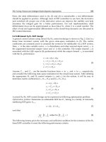
There are several ways to define a fuzzy set, in particular we define it here using the analytic
description of its membership function μ
A
(x)= f (x). For instance (see Fig. 3), the triangular
membership function can be described as:

μ
(x; a, b, c)=max

0, min

x
− a
b − a
,1,
c
− x
c −b

(11)
where a,b and c are parameters that is related to the coordinates of the triangle’s vertices,
whereas a Gaussian membership function can be described as
μ
(x; η, σ)=exp

−

x
−η
σ

2

. (12)
A static or dynamic system which makes use of fuzzy sets and the corresponding
mathematical framework is called a fuzzy system. In order to derivate the FAPI controller

−2 −1.5 −1 −0.5 0 0.5 1 1.5 2
0
0.1
0.2
0.3
0.4
0.5
0.6
0.7
0.8
0.9
1
x
μ(x)
Membership Functions


Triangular
Gaussian
Fig. 3. Example of Membership Functions: Triangular (a = −1, b = −0.5, c = 0) and
Gaussian
(η = 0.5, σ = 0.4)
updating law, it is necessary to define the intersection of fuzzy sets (connective AND),
obtained by considering a function t :
[0, 1] × [0, 1] → [0, 1] that transforms the membership
functions of fuzzy sets A and B into the membership function of the intersection of A and B,
that is:
t
[
μ

A
(x), μ
B
(x)
]
= μ
A∩B
(x). (13)
Afunctiont can be qualified as an intersection function, if it satisfies at least the following
four requirements:
t
(0, 0)=0, t (a,1)=t(1, a)=a boundary condition
t
(a, b)=t(b, a) commutativity
t
(a, b) ≤ t(a

, b

), ∀a ≤ a

, b ≤ b

monotonicity
t
(t(a, b), c)=t(a, t(b, c)) associativity
. (14)
90
Advances in PID Control
From Basic to Advanced PI Controllers: a Complexity vs. Performance Comparison 7

In the following analysis, the probabilistic connective AND will be used:
μ
A∩B
(x)=μ
A
(x)μ
B
(x). (15)
The most common fuzzy systems are defined by means of if-then rules: rule-based fuzzy
systems. In the rule-based fuzzy systems, the relationships between variables are represented
in the following general form:
if antecedent proposition then consequent proposition.
A fuzzy proposition is a statement like "x is big" where "big" is a linguistic label,definedbya
fuzzy set on the universe of discourse of variable x. In the linguistic fuzzy model developed
by [Zadeh (1978)] and [Mamdani (1977)], both the antecedent and the consequent are fuzzy
propositions:
R
i
: if x is A
i
then y is B
i
, i = 1, , L, (16)
where L is the number of propositions (rules). Here x is the input (antecedent) linguistic
variable,andA
i
are the antecedent linguistic terms (labels). Similarly, y is the output
(consequent) linguistic variable and B
i
are the consequent linguistic terms. The linguistic

terms A
i
,B
i
are always fuzzy sets. After fuzzy theory gained popularity, many control
problems have been recasted into control of Takagi-Sugeno-Kang (TSK) models:
R
i
: if xisA
i
then y = f
i
(x) , i = 1, , L (17)
which is a particular case of the general fuzzy model (16), obtained when the consequent
fuzzy sets B
i
are functions of the variable x. In systems and control theory, TSK models are
frequently used to model nonlinear systems over a fuzzy space. The resulting TSK model
can efficiently clone the nonlinear system or alternatively, approximate it over a defined
domain. For such a nonlinear systems representation, stability and synthesis of controllers
and observers can be expressed in terms of Linear Matrix Inequalities, which in turn can be
solved adopting convex optimization techniques as shown in [Tanaka (2001)]. It is important
to mention that the output of a fuzzy system can be obtained using different defuzzification
methods. In the remainder of this chapter we will use the following TSK model:
R
i
: if x
1
is A
i1

and x
n
is A
in
then y = f
i
(x) , i = 1, , L (18)
where we consider that each rule has an antecedent proposition obtained by intersecting n
fuzzy sets. The output can be evaluated by considering the Center of Gravity defuzzification
method
y
=
L
∑
i=1
α
i
f
i
(x) (19)
where
α
(t)=(α
1
(t), , α
L
(t)), α
i
(t)=
β

i
(t)
∑
L
i
=1
β
i
(t)
,
β
i
(t)=
n
∏
j=1
μ
Aij
(x). (20)
91
From Basic to Advanced PI Controllers: A Complexity vs. Performance Comparison
8 Will-be-set-by-IN-TECH
2.4.2 FAPI parameters update law
According to the discussion on fuzzy sets and rules introduced in the previous section, we
introduce now the controller parameters update laws:
IF error is SMALL, then
˙
k
p
= −β

p
k
p
(21)
IF error is MEDIUM, then
˙
k
p
= −γ
p
(k
p
−k
∗
p
) (22)
IFerrorisLARGE,then
˙
k
p
= α
p
k
∗
p
e
2
(23)
for the proportional gain k
p

, while for the integral action we have
IF error is LARGE, then
˙
k
i
= −β
i
k
i
(24)
IF error is MEDIUM, then
˙
k
i
= −γ
i
(k
i
−k
∗
i
) (25)
IF error is SMALL, then
˙
k
i
= α
i
k
∗

i
e

t
0
e(τ)dτ. (26)
The main difference with respect to the API regulator is the presence of the two terms k
∗
p
and
k
∗
i
that are the gains of a reference model regulator K
∗
. In order to compute the corresponding
time-varying gain, we will consider a single Gaussian membership function μ
S
(e) defined
over the error domain to identify the fuzzy set SMALL (S), and also the fuzzy sets MEDIUM
(M) and LARGE (L) as follows:
μ
S
= e
−
(
x
σ
)
2

, μ
L
(e)=1 − μ
S
(e), μ
M
(e)=μ
S∩L
(e)=μ
S
(e) ·μ
L
(e) (27)
The philosophy of shaping the control effort on the basis of the error value is analogous to
that of the previously introduced VIPI. The resulting k
p
gain law is obtained as
˙
k
p
=
1
1 + μ
M
(e)

α
p
μ
L

(e)k
∗
p
e
2
− β
p
μ
S
(e)k
p
−γ
p
μ
M
(e)(k
p
−k
∗
p
)

(28)
while the integral gain k
i
law is
˙
k
i
=

1
1 + μ
M
(e)

α
i
μ
S
(e)k
∗
i
e

t
0
e(τ)dτ − β
i
μ
L
(e)k
i
−γ
i
μ
M
(e)(k
i
−k
∗

i
).

(29)
Each updating law it is composed of three terms:
dissipative term

−β
p
μ
S
(e)k
p
−β
i
μ
L
(e)k
i
(30)
used to decrease the (absolute) value of the gains,
anti-dissipative term

α
p
μ
L
(e)k
∗
p

e
2
α
i
μ
S
(e)k
∗
i
e

t
0
e(τ)dτ
(31)
used to increase the gain values analogously to the API control philosophy, and
model reference tracking term

−γ
p
μ
M
(e)(k
p
−k
∗
p
)
−
γ

i
μ
M
(e)(k
i
−k
∗
i
)
(32)
92
Advances in PID Control
From Basic to Advanced PI Controllers: a Complexity vs. Performance Comparison 9
used to force the adapting law to generate controller gains sufficiently close to the ideal
controller K
∗
. In the end, the control law is as usual
u
FAPI
(t)=k
p
e(t)+k
i

t
0
e(τ)dτ (33)
In practice, when the error is large, the parameter update laws make the proportional gain
increase due to its anti-dissipative term, while the integral action progressively disappears.
This leads to a fast response (high proportional gain). On the other hand, when the error is

small, the proportional gain is subject to the dissipative term and gets negligible values, while
the integral component grows. This will result in a disturbance rejection behaviour. In any
moment, good performances are guaranteed by the third term that makes the PI close to the
model reference controller K
∗
.
Remark: Both the API controller developed in [Fisher (2009)] and the FAPI controller shown
here are not symmetrical with respect to the error signal as their update rules are a function
of the error, and thus depend on its sign. As a consequence, they can behave differently if the
reference signal is larger or smaller than the actual output of the plant.
3. Tuning methods
3.1 Tuning of the conventional PI
In this paper we tune the conventional PI using Zhuang-Atherton optimal parameters
[Zhuang and Atherton (1993)]. In particular we use the values of Table 1 of
[Zhuang and Atherton (1993)], which correspond to PI tuning formulae for set-point changes
in the case of first-order plus dead time plant model, optimised in order to minimise the
Integral of the Square Error (ISE) signal. The set-point weighting factor is usually not used
(i.e. b
= 1), as in the examples a time-varying reference signal is used.
3.2 Tuning of the VIPI
Tuning of the VIPI is a two-step procedure:
1. Conventional tuning is first performed, and values of k
p
and T
i
are found according to the
procedure outlined in Section 3.1.
2. The further parameter σ is computed to decide at which point the integral action should
come into action. Namely, the integral action must already be active when the error is
equal to the steady-state error obtained using only the proportional action.

Example :
Let us consider a plant described by the transfer function
G
(s)=
4
s
2
+ 4s + 4
(34)
and let us design a classic PI characterised by k
p
= 6.122, T
i
= 0.606 and b = 1. Then the step
response of the VIPI for different values of σ
= 0.1, 0.15, 0.25, 0.5, 1, 5 are shown in Figure 4.
As can be appreciated in Figure 4, the step response is contained between the one obtained
using a single proportional controller, which is recovered from Equation (4) when σ tends to
zero, and that of the conventional PI, which is recovered from Equation (4) when σ has large
values (in practice they coincide already for σ
= 5).
93
From Basic to Advanced PI Controllers: A Complexity vs. Performance Comparison
10 Will-be-set-by-IN-TECH
0 1 2 3 4 5 6 7 8 9 10
0
0.5
1
1.5
Time (s)

u
controller
Solid line: Conventional PI and single P
Dashed line: σ = 0.1, 0.15, 0.25, 0.5, 1, 5
Fig. 4. Different step responses as a function of the free parameter σ of the VISI. The step
response is contained between the one obtained using a single proportional controller (i.e.
σ
→ 0) and high values of the parameter. In this case, the step response when σ = 5already
coincides with the one obtained with the nominal PI.
3.3 Tuning of the API
Tuning of adaptive controllers is simpler than other PIs as the inner adaptive capacity allows
the API to recover good performances against non optimal initial tunings. However, APIs
are characterised by more degrees of freedom, e.g. parameters in the updating rules. For the
purpose of the example shown in the following sections, the adaptive PI control parameters
γ and β have been optimally tuned (using genetic algorithms) in order to get a good
trade-off between tracking and disturbance rejection. Particular care is required to handle
the anti-dissipative terms, which might yield to instability problems when a fault occurs. In
fact, the anti-dissipative term should be neglected only when the error is close to zero.
3.4 Tuning of the FAPI
The FAPI controller parameters α, β, γ must be tuned, after a desired target controller K
∗
is
chosen. In this case, we use a conventional PI tuned according to Zhuang-Atherton rules (see
Section 3.1) as a reference model. Then, the parameters can be tuned keeping in mind that
each parameter directly affects a different controller property:
• α:Adapting
• β:LowGainTrend
• γ: K
∗
Model Reference Tracking.

Therefore, parameters are chosen in function of whether the priority objective is fast response
to variations, or no overshoots or adherence to the ideal model controller. Particular care
should be used in tuning α, that should be small in presence of significative system delays.
4. Comparison of the four PIs
As a preliminary comparison the step-responses of the four controllers are compared. Then,
in the following sections, a more challenging example and a realistic scenario are simulated
to further establish the differences among the proposed PI regulators. The step response of
94
Advances in PID Control
From Basic to Advanced PI Controllers: a Complexity vs. Performance Comparison 11
the four controllers is shown in Figure 5, in the case of the system plant (34). The shown
comparison is performed after a transient time given to the adaptive controllers to adapt
their parameters, and after Zhuang-Atherton tuning procedure for the other two controllers
[Zhuang and Atherton (1993)]. The control performances of the four regulators are also
0
1 2
3
4
5 6
7
8 9
1
0
−0.2
0
0.2
0.4
0.6
0.8
1

1.2
1.4
1.6
Ti ( )
y(t)


Reference Signal
PI
VIPI
API
FAPI
Fig. 5. Comparison of the four PI controllers in terms of the step response.
compared in Table 1 to further distinguish and classify the proposed regulators, where the
following well known control indices were used
• IAE: Integral of the Absolute value of the Error, IAE
=

t
0
|
e(τ)
|
dτ
• ISE: Integral of the Square Error, ISE
=

t
0
(

e(τ)
)
2
dτ
• IAU: Integral of the Absolute value of the input u , IAU
=

t
0
|
u( τ)
|
dτ
• IADU: Integral of the Absolute value of the Derivative of the input u , IADU
=

t
0



du(τ)
dτ



dτ
IAE ISE IAU IADU
PI 0.58 0.26 16.75 22.20
VIPI 0.46 0.21 16.10 18.42

API 0.54 0.32 15.59 11.72
FAPI 0.50 0.27 15.47 8. 69
Table 1. Comparison of the four controllers in terms of the Step Response. The best values of
the indices have been highlighted in grey. The FAPI requires the least control effort, while the
VIPI has the best overall control performances.
4.1 A more challenging example
The performances of the four controllers are again compared in a more challenging scenario
where the plant transfer equation is the same (i.e. Equation (34)), but the reference signal
is composed of a periodic sinusoidal component and of a pulse wave, plus a filtered
Gaussian random signal n
(t) added to simulate sensor noise (i.e. e(t)=r(t) − y(t) − n(t)).
As a consequence, this simulation is tailored on purpose to compare the robustness and
95
From Basic to Advanced PI Controllers: A Complexity vs. Performance Comparison
12 Will-be-set-by-IN-TECH
disturbance rejection performances of the four controllers. The ability of the four controllers to
track the reference signal despite the sensor noise is shown in Figure 6. Again, the comparison
0 10 20 30 40 50 60 70
−0.8
−0.6
−0.4
−0.2
0
0.2
0.4
0.6
Time (s)
y(t)

Reference signal
PI
VIPI
API
FAPI
45 50 55 60
−0.8
−0.6
−0.4
−0.2
0
0.2
0.4
0.6
Time (s)
y(t)


Reference signal
PI
VIPI
API
FAPI
Fig. 6. Comparison of the four PI controllers in presence of a varying reference signal and
sensor noise. This simulation aims at comparing the disturbance rejection abilities of the four
controllers. On the left a long time interval, and a zoom is shown on the right. The API
exhibits the worst tracking capabilities.
has been performed after some time that was required by the adaptive controllers to reach a
steady-state behaviour. As illustrated in Figure 6, the conventional PI and the modified VIPI
apparently have the best performance in terms of tracking, however, as better shown in Figure

7, the adaptive controllers, and especially the FAPI, are characterised by a less demanding
input signal. This is particularly important because the input signal is usually required to
vary slowly in time, to avoid actuators’ stress.
Remark: In this example, the plant is required to follow small variations of the reference
signal, therefore the error is usually small and the integral action of the VIPI is constantly set
to the nominal value. As a consequence, the PI and the VIPI provide (almost) identical results.
0 10 20 30 40 50 60 70
−0.4
−0.2
0
0.2
0.4
0.6
0.8
1
Time (s)
u(t)


PI
VIPI
API
FAPI
45 50 55 60
−1
−0.5
0
0.5
Time (s)
u(t)

PI
VIPI
API
FAPI
Fig. 7. Comparison of the four PI controllers in presence of a varying reference signal and
sensor noise. This simulation shows the control effort of the four controllers. Clearly the
FAPI is the most convenient one, as actuators are less stressed. On the left a long time
interval, while on the right a shorter time interval is shown.
96
Advances in PID Control
From Basic to Advanced PI Controllers: a Complexity vs. Performance Comparison 13
4.2 A realistic example: Ship course control
Let us consider a 3DoF model of a low-speed marine vessel [Fossen (2002)]:
M
˙
ν
+ C(ν)ν + Dν = τ + J
T
(η)τ
d
(35)
˙
η
= J(η)ν (36)
where
• M represents the generalized mass-inertia matrix, including the added-masses
contribution
• C

(ν) contains the Coriolis-centripetal effects
• D represent the linear approximation of hydrodynamic drag
• τ is the generalized force-torque applied to the 3DoF model expressed in the body-fixed
reference frame
• τ
d
is an external disturbance expressed in the navigation referenceframe
• ν
=[u, v, r]
T
∈ R
3
is the state variable related to the surge, sway and yaw rate speed
• η
=[p
n
, p
e
, ψ] ∈ R
3
represents the position and the orientation of the vessel with respect
to the navigation frame
• J
(η) is the Jacobian matrix which relates body-fixed reference frame to navigation reference
frame:
J
(η)=
⎡
⎣
cos ψ

−sin ψ 0
sin ψ cos ψ 0
001
⎤
⎦
(37)
Let us assume that the vessel is moving at constant speed u
0
,and

u
2
0
+ v
2
≈ u
0
,then
the previous 3DoF model can be decoupled into longitudinal and manoeuvring subsystems.
Here we will analyse the manoeuvring subsystem in order to obtain a course control for a
vessel equipped with a single rudder. For low surge speed, in addition the Eq. (35) can be
approximated by:
¯
M
˙
¯
ν
+ N(u
0
)

¯
ν
= bδ (38)
where
¯
ν
=[v, r]
T
, b = −[Y
δ
, N
δ
]
T
∈ R
2
and
¯
M
=

m
−Y
˙
v
mx
g
−Y
˙
r

mx
g
−Y
˙
r
I
z
− N
˙
r

, N
(u
0
)=

−Y
v
mu
0
−Y
r
−N
v
mx
g
u
0
− N
r


(39)
where the parameters Y
δ
, N
δ
are used to model the force and the torque generated by the
rudder, Y
˙
v
, Y
˙
r
, N
˙
r
are parameters related to the added-masses, m, x
g
, I
z
are parameter of the
rigid-body (mass, center of gravity and moment of inertia, respectively), Y
v
, Y
r
, N
v
, N
r
are

coefficients related to the drag effects and δ is the rudder deflection. The equivalent state-space
model of (38) can be found by observing that:
˙
¯
ν
= −
¯
M
−1
N(u
0
)
¯
ν
+
¯
M
−1
bδ = A
¯
ν + Bδ (40)
Considering the the parameters of the CyberShip II experimentally estimated in Fossen (2004),
choosing a constant speed of u
0
= 1.5m/s ≈ 3kno ts and defining the output y = r =
97
From Basic to Advanced PI Controllers: A Complexity vs. Performance Comparison
14 Will-be-set-by-IN-TECH
C
r

¯
ν, C
r
=[0, 1] ∈ R
2
, the following second linear time invariant system, also referred as
Nomoto 2nd order model is obtained:
G
r
(s)=C
r
(
sI − A
)
−1
B =
r(s)
δ(s)
=
−
0.09185s −0.002137
s
2
+ 0.8165s + 0.04882
(41)
Since the course angle derivative is related to the yaw-rate as
˙
ψ
= r, we can finally derive the
course model for the CyberShip II as:

G
ψ
(s)=
ψ( s)
δ(s)
=
1
s
G
r
(s)=
−
0.09185s −0.002137
s
3
+ 0.8165s
2
+ 0.04882s
(42)
The controller parameters used in the course-control problem are summarised in Table 2.
ZA VIPI API FAPI
K
∗
p
7.7220 7.7220 - 7.7220
K
∗
i
= K
∗

p
/T
∗
i
0.0978 0.0978 - 0.0978
σ - 0.5 - 0.25
β
p
- - 1.1612 0.0087
β
i
- - 1.1343 0.1206
γ
p
- - 0.0151 0.1142
γ
i
- - 0.1363 0.1671
α
p
- - - 0.0011
α
i
- - - 0.7126
Table 2. Course Control Problem: controller parameters used in the simulation.
Note that we are not handling actuator saturations and limitations of the input rate.
However, in order to use efficiently those controllers with such limitations the adoption of
anti-windup systems and reference filters is strongly recommended. In practice, the use of
a frequency-shaped reference signal causes a smoother and less demanding control action
which is expected to satisfy the actuator limitations.

The four controllers are compared in the challenging scenario described in Figure 8. In this
simulation we assume that the reference signal is a desired course angle (i.e. not a step
reference, as it is not realistic in this context as previously remarked). Disturbance is modeled
with two components: a filtered Gaussian noise, of the order of 2
−3
◦
; and an aperiodic square
pulse which refers to unpredictable external disturbance (e.g. wave current, wind gust). It
is possible to note from Figure 8 that the API controller not always provide a satisfactory
tracking of the reference signal. On the other hand, the other controllers have similar good
performances, but the FAPI is characterised by a reduced control effort.
5. Conclusion
This chapter gives a comparison between a conventional PI regulator tuned according to
Zhuang-Atherton rules with three less conventional controllers: a variable integral component
PI (VIPI), an adaptive PI (API) and a fuzzy adaptive PI (FAPI). The VIPI is characterised by
one time variant parameter, i.e. the integral one, and only one more degree of freedom (the
parameter σ). Both the API and the FAPI have two time variant parameters and more degrees
of freedom, as for instance the dissipative and anti-dissipative coefficients that regulate the
parameters’ update laws.
98
Advances in PID Control
From Basic to Advanced PI Controllers: a Complexity vs. Performance Comparison 15
0 20 40 60 80 100 120 140
−30
−20
−10
0
10
20
30

40
50
Time (s)
Course Angle ψ (deg)


Reference signal
PI
VIPI
API
FAPI
0 20 40 60 80 100 120 140
−80
−60
−40
−20
0
20
40
60
80
Time(s)
Rudder Deflection δ(t) (deg)


PI
VIPI
API
FAPI
Fig. 8. Comparison of the four PI controllers in response to a course angle reference signal

(on the left). Realistic disturbances are taken into consideration. On the right, the control
effort of the four controllers.
Simulations show that the VIPI generally outperforms the simple PI both in terms of the
control effort, which is always inferior, and in terms of settling time. The VIPI is very
convenient, as it only contains one more parameter than the conventional PI, and better
performances are usually achieved without requiring a complex tuning procedure for the
extra parameter. On the other hand, the adaptive controllers require a more laborious tuning
procedure (as more parameters are involved), and not always the control performance is
so satisfactory, especially for the API, at least for the proposed examples. However, the
FAPI, although provides similar control results to the PI and the VIPI, is characterised by a
reduced small effort, both in terms of the absolute value and its derivative; for this reason it is
particularly suitable in particular control applications: for instance when control components
with moving parts are involved (e.g. valves) frequent fluctuations of the control action should
be avoided to skip the high expenses of valve wear and maintenance programs.
Ongoing and future work will follow several directions:
• Robustness performances will be further investigated, so to account for time variant
process plants. In some industrial applications, the plant coefficients change according
to different factors (e.g. temperature, age, wear and tear of the machines).
• The controllers can be further compared on their ability to prevent wind-up phenomena.
• The proposed framework can be easily extended to decentralised Multiple Input Multiple
Output (MIMO) control problems.
• The FAPI controller exhibits the best performance in terms of control effort, and for this
reason it will be used in a real application in underwater robotics.
6. References
E. Sperry, Automatic steering, Society of Naval Architects and Marine Engineers, 1922.
N. Minorski, Directional stability of automatically steered bodies, Journal of American Society of
Naval Engineers, 1922.
J. Ziegler and N. Nichols, Optimum settings for automatic controller, Trans. ASME, vol. 75,
pp.827–833, 1942.
K. Astrom and E. Hagglund, Adaptive tuning of simple regulators with specifications on phase and

amplitude mar gins, Automatica, vol. 20, pp. 645–651, 1984.
99
From Basic to Advanced PI Controllers: A Complexity vs. Performance Comparison
16 Will-be-set-by-IN-TECH
M. Zhuang and D.P. Atherton, Automatic tuning of optimum PID controllers, IEE Proceedings D
on Control Theory and Applications, vol. 140, pp. 216–224, 1993.
W. Luyben and E. Eskinat, Nonlinear auto-tune identification, International Journal of Control,
vol. 59, pp.595–626, 1994.
H. Rasmussen, Automatic tuning of pid-regulators, Textbook, Department of Control
Engineering, Aalborg University, Denmark, 2009.
Y. Peng, D. Vrancic and R. Hanus, Anti-windup, bumpless, and CT techniques for PID controllers,
IEEE Control systems magazine, vol. 16, pp.48–56, 1996.
K.Tang,K.Man,G.ChenandS.Kwong,An optimal fuzzy PID controller, IEEE Transactions on
Industrial Electronics, vol. 48, pp. 757–765, 2001.
A. Visioli, A new design for a PID plus feedforward controller, Journal of Process Control, vol. 14,
pp. 457–463, 2004.
A. Haj-Ali and H. Ying, Structural analysis of fuzzy controllers with nonlinear input fuzzy sets in
relation to nonlinear PID control with variable gain, Automatica, vol. 40, pp. 1551–1559,
2004.
A. Scottedward Hodel and C.E. Hall, Variable-Structure PID control to prevent in tegrator windup,
IEEE Transactions on Industrial Electronics, vol. 48, no. 2, 2001.
A. Visioli, Fuzzy logic based set-point weight tuning of PID controllers, IEEE Transactions on
Systems, Man, and Cybernetics - Part A, vol. 29, no. 6, pp. 587–592, 1999.
A. Leva and M. Maggio, A systematic way to extend ideal PID tuning rules to the real structure,
Journal of Process Control, vol. 21, pp. 130–136, 2011.
A. Balestrino, V. Biagini, P. Bolognesi and E. Crisostomi, Advanced variable structure PI
controllers, IEEE Conference on Emerging Technologies and Factory Automation
(ETFA), 2009.
A.D. Fisher, J.H. VanZwieten and T.S. VanZwieten, Adaptive Control of Small Outboard-Powered
Boats for Survey Applications, OCEANS 2009, MTS/IEEE Biloxi - Marine Technology

for Our Future: Global and Local Challenges, 2009.
L.X. Wang, A Course in Fuzzy Systems and Control, Prentice Hall,1997.
L.A. Zadeh, Fuzzy Sets as basis for a theory of possibility., Fuzzy Sets and System 1, 1978.
E.H. Mamdani, Application of Fuzzy Logic to Approximate Reasoning Using Linguistic Synthesis,
IEEE Transaction on Computers, 1977.
K. Tanaka and H.O. Wang, Fuzzy Control Systems Design and Analysis: A Linear Matrix Inequality
Approach, John Wiley and Sons, 2001.
T.I. Fossen, Marine Control Systems: Guidance, Navigation and Control of Ships, Rigs and
Underwater Vehicles, Marine Cybernetics, 2002.
T. I. Fossen, Modeling, Identification, and Adaptive Maneuvering of CyberShip II: A complete design
with experiments, Proc. of the IFAC CAMS’04, Ancona, Italy.
100
Advances in PID Control
0
Adaptive Gain PID Control for
Mechanical Systems
Ricardo Guerra, Salvador González and Roberto Reyes
Universidad Autónoma de Baja California
México
1. Introduction
The design and use of PID controllers is a part of what has been denominated Classical
Control, which as the name implies, has been studied for many years (DiStefano et al. 1996),
however it continues to be a source for research (Alvarez et al. 2008), (Ang et al. 2008),
(Su et al. 2010).
The structure of the controller contains a differential term to aid in the reduction of system
friction and an integral term to attenuate steady state error. The drawbacks of this control
scheme, particularly for nonlinear mechanical systems, include the difficulty in selecting
adecuate controller gains, a process usually refered to as tuning. The difficulty usually lies in
the fact that if the controller gains are set too small, the control objective may never be reached,
whereas the selection of excesively large controller gains may result in system instability.

Many approaches have been proposed to properly tune PID gains (Ang et al. 2008),
(Chang & Jung 2009), (Su et al. 2010), others have tried to improve upon the performance
of the PID controller by including modern control techniques such as neural networks, fuzzy
logic or variable structure control (Guerra et al. 2005).
Among these, variable structure control, specifically sliding mode control, has shown
to possess certain desirable properties, such as disturbance rejection and finite time
convergence; however it also presents unwanted behaviors mainly high frequency switching,
a phenomenon refered to as chattering, which is undesirable in mechanical systems because
it can cause accelerated wear of the mechanical components as well as activate unmodeled
dynamics. One solution presented is to include an adaptive gain in the high frequency term
so that the desirable properties may be exploited, and the undesirable effects minimized,
achieving an enhanced performance (Guerra et al. 2005).
2. Background
The control of mechanical systems is subject to many difficulties, as evidenced by the research
devoted to such aspects of mechanical systems as dead zone (Zhang & Gen 2009), and friction
(Canudas de Wit et al. 1995).
Consider a first order mechanical system given by (Canudas de Wit et al. 1995)
6
2 .
¨
x
=
u − f
(
˙
x
)
m
(1)
where x is the position variable, m is the mass, u is the control input and the

function f
(
˙
x
) denotes the nonlinear friction force. The PID control law is given by
(Canudas de Wit et al. 1995):
u
= K
p
e + K
i

t
0
e(τ)dτ + K
d
˙
e (2)
where K
p
, K
d
and K
i
, are the proportional, derivative and integral gains, respectively and the
error term is given by e
= x − x
d
,wherex
d

is the constant desired value.
Mechanical systems under integral control action have been known to present limit cycles, due
in part to the complex nature of the friction force. This results in the system never reaching
the desired position (Canudas de Wit et al. 1995).
The authors in (Guerra et al. 2005) present an approach considering a PD controller which
is modified by the inclusion of a neural networks chattering controller that allows the high
frequency swithching when the system is away from the desired position, but tends to vanish
once the desired position is reached. In this chapter we will build upon that result and apply
a similar stragegy to a PID controller.
3. Controller design
Consider the system (1) with unit mass and friction force given by (Makkar et al. 2005):
f
(
˙
x
)
=
γ
1
[
tanh
(
γ
2
˙
x
)
−
tanh
(

γ
3
˙
x
)]
+
γ
4
tanh
(
γ
5
˙
x
)
+
γ
6
˙
x (3)
The objective is for the error e to reach zero, i.e. ,:
lim
t→∞
e(t)=0(4)
where
e
= x − x
d
(5)
to achieve this, the controller (2) is modified to:

u
= −K
p
e − K
i
ζ − [2ε + δK
d
]
˙
e (6)
where
˙
ζ
= e (7)
˙
δ
= −α ln(δ + 1)+K
r
[δ + 1]
ln(δ + 1)+1
e
2
(8)
where ε
> 0, α > 0andK
r
> 0 are constant parameters. The term ζ is used for simplicity in
place of the term

t

0
e(τ)dτ. It should be noted that for an intnitial condition δ(t
0
)=δ
0
≥ 0,
δ
(t) ≥ 0, for all t ≥ t
0
(Hench, 1999). In addtion, the adaptive gain can be considered to be
bound by δ
≤ δ
M
by taking into account that a practical controller is subject to saturation.
102
Advances in PID Control
Adaptive Gain PID Control for
Mechanical Systems 3
4. Closed loop system
To analyze the stability of the closed loop system, the following variable change is introduced:
ω
= εζ + e (9)
which is used to form the vector ξ
=
[
ω e
˙
e
]
T

. Using equations (1), (3), (5), (6) and (7) the
dynamic of the closed loop system is given by:
˙
ξ
= A(δ)ξ + B(
˙
e
) (10)
where
A
(δ)=
⎡
⎣
0 ε 1
00 1
−ε
−1
K
i
−

K
p
−ε
−1
K
i

−
[

2ε + δK
d
]
⎤
⎦
(11)
B
(
˙
e
)=[00− f (
˙
e
)]
T
(12)
The state δ contained in A
(δ)
3,3
is governed by the dynamic adaptation law (8). By setting (8)
and (10) to zero, it can be seen that the origin of the state space (ξ
= 0, δ = 0) is the unique
equillibrium for the system which, when applied to equation (9), implies ζ
= 0.
5. Stability analysis
Consider the candidate Lyapunov function:
V
(ξ, δ)=ξ
T
P

c
ξ +(δ + 1) ln(δ + 1) (13)
where
P
c
=
1
2

P
+ P
T

(14)
P
=
⎡
⎣
βε
−1
K
i
00
0 β

K
p
−ε
−1
K

i

0
02βε β
⎤
⎦
(15)
It should be noted that V
> 0 implies that P
c
> 0, which by applying Sylvester’s Theorem
(Kelly et al. 2005) requires that β
> 0, the complete analysis to ensure positivity of matrix P
c
is presented in the next section. To simplify stability analysis, the equality ξ
T
P
c
ξ = ξ
T
Pξ is
considered so that expression (13) can be restated as
V
(ξ, δ)=ξ
T
Pξ +(δ + 1) ln(δ + 1) (16)
The time derivative of (16) along the closed loop system (8) and (10) yields:
˙
V
= −ξ

T
Q(δ)ξ −R(ξ) − α ln( δ + 1)[ln( δ + 1)+1] (17)
where
R
(ξ)=−B(
˙
e
)
T
Pξ − ξ
T
PB(
˙
e
)=2 βεef(
˙
e
)+2β
˙
ef(
˙
e
) (18)
103
Adaptive Gain PID Control for Mechanical Systems
4 .
W(δ)=−

PA
(δ)+A(δ )

T
P

(19)
Q
(δ)=
1
2

W
(δ)+W(δ)
T

−
ˆ
e
2
K
r
(δ + 1)
ˆ
e
T
2
=
⎡
⎣
00 0
02βε


K
p
−ε
−1
K
i

−K
r
(
δ + 1
)
βε
[
2ε + δK
d
]
0 βε
[
2ε + δK
d
]
2β
[
ε + δK
d
]
⎤
⎦
(20)

where
ˆ
e
2
=[010]
T
. Regarding equation (3) used in (18), every term in the expression can
be bound by b tanh
(c) ≤|b||c|∀b, c ∈. It can be stated that equation (3) satisfies:
−ef(
˙
e
) ≤ K
γ
|e||
˙
e
| (21)
where
K
γ
= γ
1
|γ
2
−γ
3
|+ γ
4
γ

5
+ γ
6
(22)
it should be remembered that all the parameters γ
ι
for ι = 1 . . . 6 are positive constants.
Regarding the term
˙
ef
(
˙
e
) in equation (18), it can be seen that this term is positive for
γ
2
≥ γ
3
> 0 by using the properties of hiperbolic functions in equation (3) and considering
˙
e
→ Θ ≥ 0 (first quadrant) we find that:
tanh
(
[
γ
2
−γ
3
]Θ

)[
1 −tanh
(
γ
2
Θ
)
tanh
(
γ
3
Θ
)]
≥
0 (23)
given that Θ, γ
2
and γ
3
are considered to be positive, the second term will always be non
negative, whereas the first will be non negative if γ
2
≥ γ
3
> 0 (as was previously stated).
These considerations apply also when
˙
e
→ Θ ≤ 0 (third quadrant). By applying (21), (22) and
(23) in (18), along with the previously stated δ

≤ δ
M
equation (17) can be bounded by:
˙
V
≤−

|e|
|
˙
e
|

T
Q
c

|e|
|
˙
e
|

−2β
˙
ef(
˙
e
) − α ln(δ + 1)
[

ln(δ + 1)+1
]
(24)
where
Q
c
=

2βε

K
p
−ε
−1
K
i

−K
r
(
δ
M
+ 1
)
βε
(
2ε + δ
M
K
d

−K
γ
)
βε
(
2ε + δ
M
K
d
−K
γ
)
2βε

(25)
In the follwing section, a process for tuning the controller gains will be introduced, this will
also be useful in provinding sufficient conditions to guarantee the positiviy of matrices P
c
and
Q
c
.
6. Controller tuning
In order to establish bounds on the controller gains, we first analyze the matrix P
c
defined
in expression (14). To find the roots of this symmetric matrix, we apply Sylvester’s Theorem
(Kelly et al. 2005), which generates a cubic polynomial of the form ε
3
− 3bε + 2a < 0with

a
=
K
i
2
and b =
K
p
3
which is satisfied for b
3
> a
2
.Usingexp(•) to denote the exponential
function, we define the terms υ
1,2
= −a ± ic = r exp
[
∓
i
(
θ − π
)]
, c =
√
b
3
− a
2
, r = b

3
2
,
θ
= arctan

c
a

, ϑ
1,2
= 2a + υ
1,2
= r exp
(
±
iθ
)
and using Euler’s formula the roots are:
104
Advances in PID Control
Adaptive Gain PID Control for
Mechanical Systems 5
ε
1
= −
(
p
1
+ p

2
)
= −
2r
1
3
cos

θ
3

(26)
ε
2
=
√
y
1
y
2
= 2r
1
3
sin

π
−2θ
6

(27)

ε
1
= q
1
+ q
2
= 2r
1
3
cos

π
−θ
3

(28)
considering that p
ι
= ϑ
1
3
ι
, q
ι
= υ
1
3
ι
,andy
ι

= p
ι
− q
ι
for ι = 1, 2. Given that
c
∈
+
, θ ∈

0,
π
2

.Takingthenε
1
< 0, and 0 < ε
2
≤ ε
3
. The polynomial
ε
3
− 3bε + 2a =
(
ε − ε
1
)(
ε −ε
2

)(
ε −ε
3
)
<
0 is satisfied for all ε
2
< ε < ε
3
.
We propose the definition b
3
=

σ
2
+ 1

a
2
with σ  0, in other words, the proportional gain
in equation (6) is tuned as
K
p
=

27K
2
i
4


σ
2
+ 1


1
3
(29)
Returning to Q
c
defined in expression (25), this matrix can be defined as positive by applying
Sylvester’s Theorem (Kelly et al. 2005) and tuning the derivitave gain in (6) as
K
d
=
K
γ
−2ε
δ
M
(30)
the numerator in this equation must be positive, specifically, the constant bound from
equation (22) must satisfy K
γ
> 2ε, so from equations (26)-(30) the positivity of matrices P
c
and Q
c
is restricted to

max

K
i
K
p
,
2βK
i
+ K
r
(δ
M
+ 1)
2βK
p
, ε
2

< ε < mi n

K
γ
2
, ε
3

(31)
By establishing conditions to satisfy (31), which include the values of K
r

and K
i
selected to
generate a valid range for ε, we can conclude that expression (13) is positive definite and
that expression (17) is locally negative semi-definite, consequently the system (8) and (10)
has a stable equilibrium at the origin. Moreover, by restricting η
=

ξ
T
δ

T
by the bounds
η
min
≤ η ≤ η
max
and applying LaSalle’s Principle (Kelly et al. 2005) to expression (24) a
closed set can be defined as:
Ω
= {η ∈
4
:
˙
V
(
η
)
=

0} = {ω ∈,
[
e
˙
e δ
]
T
= 0} (32)
Solving (32) along (8) and (10) it can be seen that
lim
t→∞
ω(t)=0 (33)
and by invoking the variable change (9) that
lim
t→∞
ζ( t)=0 (34)
therefore the origin of the system defined by (8) and (10) is locally asymptotically stable.
105
Adaptive Gain PID Control for Mechanical Systems
6 .
7. Simulation results
In order to test the performance of the proposed controller simulations were carried out using
the friction model (3) with the parameters set to γ
1
= 1.25, γ
2
= 100, γ
3
= 10, γ
4

= γ
5
= 1.,
γ
6
= 0.1, α = 10, β = 1, δ
M
= 1, σ = 100, K
i
= K
r
= 10 and the mass is considered to be
unitary.
Using the mentioned values in equations (22), (29) and (30) we obtain K
p
= 188.9945,
K
γ
= 122.6 and applying the obtained values to equation (31) we arrive at
max
{0.53, 0.106, 0.52 } < ε < min { 61.3, 13.7 } such that the value chosen was ε = 6.808
and hence K
d
= 108.9848.
Figure 1 shows the performance of the position regulation. It should be noted that there is
a very small overshot and that no limit cycles are present. The asymptotic stability can be
easily seen in Figure 2 where the error is presented, it is clear that the error is still decreasing,
achieving an accuracy within a micrometer after 200 seconds.
0 50 100 150 200
0

0.2
0.4
0.6
0.8
1
1.2
1.4
Time [seconds]
Position [meters]
Fig. 1. Controller Performance: Achieved Position.
Figure 3 shows the evolution of the adaptive gain δ, it is clear that as the error approaches
zero, so too does the value of the adaptive gain, and consequently so does the value of the
controlvariable,showninFigure4.
The control variable initially presents a large value which then decreases. It can be inferred
from the asymptotic stability that the control variable decreses asymptotically with time as
shown in Figures 4 and 5. Figure 5 shows the control variable in more detail. During the first
ten seconds a small oscillation can be seen but it is eliminated after approximately 3 seconds.
Figures 6 and 7 show that the term ζ
=

t
0
e(τ)dτ also approaches zero. It can be clearly seen,
especially in Figure 7 that ζ asymptotically approaches zero.
106
Advances in PID Control
Adaptive Gain PID Control for
Mechanical Systems 7
195.5 196 196.5 197 197.5 198 198.5 199 199.5 200
4.5

5
5.5
6
6.5
7
7.5
8
x 10
−7
Time [seconds]
Position error [meters]
Fig. 2. Controller Performance: Position Error.
0 50 100 150 200
0
0.5
1
1.5
Time [seconds]
Magnitude of the adaptive gain δ
Fig. 3. Controller Performance: Adaptive Gain.
107
Adaptive Gain PID Control for Mechanical Systems
8 .
0 50 100 150 200
−50
0
50
100
150
200

Time [seconds]
Control Variable
Fig. 4. Controller Performance: Control Variable.
0 2 4 6 8 10
−50
0
50
100
150
200
Time [seconds]
Control Variable
Fig. 5. Controller Performance: Control Variable (detail).
108
Advances in PID Control