Advances in PID Control Part 7 ppt

Adaptive Gain PID Control for
Mechanical Systems 9
0 50 100 150 200
−0.5
−0.45
−0.4
−0.35
−0.3
−0.25
−0.2
−0.15
−0.1
−0.05
0
Time [seconds]
Error integral
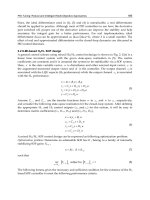
Fig. 6. Controller Performance: Error Integral.
195.5 196 196.5 197 197.5 198 198.5 199 199.5 200
−12
−10
−8
−6
−4
−2
0
x 10
−6
Time [seconds]
Error integral
Fig. 7. Controller Performance: Error Integral (detail).
109

Adaptive Gain PID Control for Mechanical Systems
10 .
Figure 8 shows how with increasing time, the value of the adaptive gain draws even closer to
zero. The same can be said of the error in Figure 9 and of ζ in Figure 10.
395.5 396 396.5 397 397.5 398 398.5 399 399.5 400
−1.5
−1
−0.5
0
0.5
1
x 10
−16
Time [seconds]
Magnitude of the adaptive gain δ
Fig. 8. Controller Performance: Adaptive Gain (detail).
395.5 396 396.5 397 397.5 398 398.5 399 399.5 400
0
0.5
1
1.5
2
2.5
x 10
−11
Time [seconds]
Position error [meters]
Fig. 9. Controller Performance: Position Error (detail).
110
Advances in PID Control

Adaptive Gain PID Control for
Mechanical Systems 11
390 392 394 396 398 400
−3
−2
−1
0
x 10
−10
Time [seconds]
Error integral
Fig. 10. Controller Performance: Error Integral (detail).
8. Conclusions
An extension to the traditional PID controller has been presented that incorporates an
adaptive gain. The adaptive gain PID controller presented is demonstrated to asymptotically
stabilize the system, this is shown in the simulations where the position error converges to
zero.
In the presented analysis, considerations using known bounds of the system (such as friction
coefficients) are used to show the stability of the system as well as to tune the controller gains
K
p
and K
d
.
9. References
Alvarez, J.; Santibañez, V. & Campa, R. (2008). Stability of Robot Manipulators Under
Saturated PID Compensation. IEEE Transactions on Control Systems Technology,Vol.
16, No. 6, Nov 2008, 1333 – 1341, ISSN 1063-6536
Ang, K. H.,; Chong, G. & Li, Y. (2005). PID Control System Analysis, Design, and Technology.
IEEE Transactions on Control Systems Technology, Vol. 13, No. 4, Jul 2005, 559 – 576,

ISSN 1063-6536
Canudas de Wit, C. ; Olsson, H. ; Astrom, K.J. & Lischinsky, P. (1995). A new model for control
of systems with friction. IEEE Transactions on Automatic Control, Vol. 40, No. 3, Mar
1995, 419 – 425, ISSN 0018-9286
Chang, P. H. & Jung J.H. (2009). A Systematic Method for Gain Selection of Robust PID Control
for Nonlinear Plants of Second-Order Controller Canonical Form. IEEE Transactions
on Automatic Control, Vol. 17, No. 2, Mar 2009, 473 – 483, ISSN 1063-6536
111
Adaptive Gain PID Control for Mechanical Systems
12 .
Distefano, J. J.; Stuberud, A. R & Williams, I. J.(1990). Feedback and Control Systems, 2nd Edition,
McGraw Hill, ISBN: 0-13228024-8, Upper Saddle River, New Jersey.
Guerra, R.; Acho, L. & Aguilar L.(2005). Chattering Attenuation Using
Linear-in-the-Parameter Neural Nets in Variable Structure Control of Robot
Manipulators with friction . Proceedings of the International Conference on Fuzzy
Systems and Genetic Algorithms 2005, pp. 65 – 75, Tijuana, Mexico, October 2005.
Hench, J. J. (1999). On a class of adaptive suboptimal Riccati-based controllers. Proceedings of
the : American Control Conference, 1999., pp. 53 – 55, ISBN: 0-7803-4990-3 , San Diego,
CA, June 1999.
Kelly, R.; Santibáñez, V. & Loría, A. (1996). Control of Robot Manipulators in Joint Space,Springer,
ISBN: 978-1-85233-994-4, Germany.
Makkar, C.; Dixon, W.E.; Sawyer, W.G. & Hu, G. (2005). A new continuously differentiable
friction model for control systems design. Proceedings of the 2005 IEEE/ASME
International Conference on Advanced Intelligent Mechatronics, pp. 600 – 605, ISBN:
0-7803-9047-4, Monterey, CA, July 2005.
Su, Y.; Müller P. C. & Zheng, C. (2010). Global Asymptotic Saturated PID Control for Robot
Manipulators. IEEE Transactions on Control Systems Technology,Vol.18,No.6,Nov
2010, 1280 – 1288, ISSN 1063-6536
Zhang, T. & Ge, S. S. (2009). Adaptive Neural Network Tracking Control of MIMO Nonlinear
Systems With Unknown Dead Zones and Control Directions. IEEE Transactions on

Neural Networks, Vol. 20, No.3, Mar 2009, 483 – 497, ISBN 1045-9227
112
Advances in PID Control
0
PI/PID Control for Nonlinear Systems
via Singular Perturbation Technique
Valery D. Yurkevich
Novosibirsk State Technical University
Russia
1. Introduction
The problem of output regulation for nonlinear time-varying control systems under
uncertainties is one of particular interest for real-time control system design. There is a broad
set of practical problems in the control of aircraft, robotics, mechatronics, chemical industry,
electrical and electro-mechanical systems where control systems are designed to provide the
following objectives: (i) robust zero steady-state error of the reference input realization; (ii)
desired output performance specifications such as overshoot, settling time, and system type of
reference model for desired output behavior; (iii) insensitivity of the output transient behavior
with respect to unknown external disturbances and varying parameters of the system.
In spite of considerable advances in the recent control theory, it is common knowledge that
PI and PID controllers are most widely and successfully used in industrial applications
(Morari & Zafiriou, 1999). A great attention of numerous researchers during the last
few decades was devoted to turning rules (Åström & Hägglund, 1995; O’Dwyer, 2003;
Ziegel & Nichols, 1942), identification and adaptation schemes (Li et al., 2006) in order to
fetch out the best PI and PID controllers in accordance with the assigned design objectives.
The most recent results have concern with the problem of PI and PID controller design
for linear systems. However, various design technics of integral controllers for nonlinear
systems were discussed as well (Huang & Rugh, 1990; Isidori & Byrnes, 1990; Khalil, 2000;
Mahmoud & Khalil, 1996). The main disadvantage of existence design procedures of PI or
PID controllers is that the desired transient performances in the closed-loop system can not
be guaranteed in the presence of nonlinear plant parameter variations and unknown external

disturbances. The lack of clarity with regard to selection of sampling period and parameters
of discrete-time counterparts for PI or PID controllers is the other disadvantage of the current
state of this question.
The output regulation problem under uncertainties can be successfully solved via such
advanced technics as control systems with sliding motions (Utkin, 1992; Young & Özgüner,
1999), control systems with high gain in feedback (Meerov, 1965; Young et al., 1977). A set
of examples can be found from mechanical applications and robotics where acceleration
feedback control is successfully used (Krutko, 1988; 1991; 1995; Lun et al., 1980; Luo et al.,
1985; Studenny & Belanger, 1984; 1986). The generalized approach to nonlinear control system
design based on control law with output derivatives and high gain in feedback, where
integral action can be incorporated in the controller, is developed as well and one is used
7
PI/PID Control for Nonlinear Systems
via Singular Perturbation Technique 1
effectively under uncertainties (Błachuta et al., 1997; 1999; Czyba & Błachuta, 2003; Yurkevich,
1995; 2004). The distinctive feature of such advanced technics of control system design is
the presence of two-time-scale motions in the closed-loop system. Therefore, a singular
perturbation method (Kokotovi´c et al., 1976; 1999; Kokotovi´c & Khalil, 1986; Naidu & Calise,
2001; Naidu, 2002; Saksena et al., 1984; Tikhonov, 1948; 1952) should be used for analysis of
closed-loop system properties in such systems.
The goal of the chapter is to give an overview in tutorial manner of the newest unified design
methodology of PI and PID controllers for continuous-time or discrete-time nonlinear control
systems which guarantees desired transient performances in the presence of plant parameter
variations and unknown external disturbances. The chapter presents the up-to-date coverage
of fundamental issues and recent research developments in singular perturbation technique
of nonlinear control system design. The discussed control law structures are an extension
of PI/PID control scheme. The proposed design methodology allows to provide effective
control of nonlinear systems on the assumption of uncertainty, where a distinctive feature
of the designed control systems is that two-time-scale motions are artificially forced in
the closed-loop system. Stability conditions imposed on the fast and slow modes, and a

sufficiently large mode separation rate, can ensure that the full-order closed-loop system
achieves desired properties: the output transient performances are as desired, and they
are insensitive to parameter variations and external disturbances. PI/PID control design
methodology for continuous-time control systems, as well as corresponding discrete-time
counterpart, is discussed in the paper. The method of singular perturbations is used to analyze
the closed-loop system properties throughout the chapter.
The chapter is organized as follows. First, some preliminary results concern with properties of
singularly perturbed systems are discussed. Second, the application of the discussed design
methodology for a simple model of continuous-time single-input single-output nonlinear
system is presented and main steps of the design method are explained. The relationship
of the presented design methodology with problem of PI and PID controllers design for
nonlinear systems is explained. Third, the discrete-time counterpart of the discussed design
methodology for sampled-data control systems design is highlighted. Numerical examples
with simulation results are included as well.
The main impact of the chapter is the presentation of the unified approach to continuous
as well as digital control system design that allows to guarantee the desired output
transient performances in the presence of plant parameter variations and unknown external
disturbances. The discussed design methodology may be used for a broad class of nonlinear
time-varying systems on the assumption of incomplete information about varying parameters
of the plant model and unknown external disturbances. The advantage of the discussed
singular perturbation technique for closed-loop system analysis is that analytical expressions
for parameters of PI, PID, or PID controller with additional lowpass filtering can be found for
nonlinear systems, where controller parameters depend explicitly on the specifications of the
desired output behavior.
2. Singularly perturbed systems
2.1 Continuous-time singularly perturbed systems
The singularly perturbed dynamical control systems arise in various applications mainly due
to two reasons. The first one is that fast dynamics of actuators or sensors leads to the plant
114
Advances in PID Control

2 Will-be-set-by-IN-TECH
model in the form of singularly perturbed system (Kokotovi´c et al., 1976; Naidu & Calise,
2001; Naidu, 2002; Saksena et al., 1984). The second one is that the singularly perturbed
dynamical systems can also appear as the result of a high gain in feedback (Meerov, 1965;
Young et al., 1977). In accordance with the second one, a distinctive feature of the discussed
control systems in this chapter is that two-time-scale motions are artificially forced in the
closed-loop control system due to an application of a fast dynamical control law or high gain
parameters in feedback.
The main notions of singularly perturbed systems can be considered based on the following
continuous-time system:
˙
X
= f (X, Z),(1)
μ
˙
Z
= g(X, Z),(2)
where μ is a small positive parameter, X
∈ R
n
, Z ∈ R
m
,and f and g are continuously
differentiable functions of X and Z. The system (1)–(2) is called the standard singularly
perturbed system (Khalil , 2002; Kokotovi´c et al., 1976; 1999; Kokotovi´c & Khalil, 1986).
From (1)–(2) we can get the fast motion subsystem (FMS) given by
μ
dZ
dt
= g (X, Z) (3)

as μ
→ 0whereX(t) is the frozen variable. Assume that
det

∂g
(X, Z)
∂Z

= 0(4)
for all Z
∈ Ω
Z
where Ω
Z
is the specified bounded set Ω
Z
⊂ R
m
.
From (4) it follows that the function
¯
Z
= ψ(X) exists such that g(X(t),
¯
Z(t)) = 0 ∀ t holds
where
¯
Z is an isolated equilibrium point of (3). Assume that the equilibrium point
¯
Z is unique

and one is stable (exponentially stable).
After the fast damping of transients in the FMS (3), the state space vector of the system (1)–(2)
belong to slow-motion manifold (SMM) given by
M
smm
= {(X, Z) : g(X, Z)=0}.
By taking μ
= 0, from (1)–(2), the slow motion subsystem (SMS) (or a so-called reduced
system) follows in the form
˙
X
= f (X, ψ(X)).
2.2 Discrete-time singularly perturbed systems
Let us consider the system of difference equations given by
X
k+1
= {I
n
+ μA
11
}X
k
+ μA
12
Y
k
,(5)
Y
k+1
= A

21
X
k
+ A
22
Y
k
,(6)
where μ is the small positive parameter, X
∈ R
n
, Y ∈ R
m
,andtheA
ij
are matrices with
appropriate dimensions.
115
PI/PID Control for Nonlinear Systems via Singular Perturbation Technique
PI/PID Control for Nonlinear Systems
via Singular Perturbation Technique 3
If μ is sufficiently small, then from (5)–(6) the FMS equation
Y
k+1
= A
21
X
k
+ A
22

Y
k
(7)
results, where X
k+1
−X
k
≈ 0 (that is X
k
≈ const) during the transients in the system (7).
Assume that the FMS (7) is stable. Then the steady-state of the FMS is given by
Y
k
= {I
m
− A
22
}
−1
A
21
X
k
.(8)
Substitution of (8) into (5) yields the SMS
X
k+1
= {I
n
+ μ[A

11
+ A
12
(I
m
− A
22
)
−1
A
21
]}X
k
.
The main qualitative property of the singularly perturbed systems is that: if the equilibrium
point of the FMS is stable (exponentially stable), then there exists μ

> 0suchthatforall
μ
∈ (0, μ

), the trajectories of the singularly perturbed system approximate to the trajectories
of the SMS (Hoppensteadt, 1966; Klimushchev & Krasovskii, 1962; Litkouhi & Khalil, 1985;
Tikhonov, 1948; 1952). This property is important both from a theoretical viewpoint and for
practical applications in control system analysis and design, in particular, that will be used
throughout the discussed below design methodology for continuous-time or sampled-data
nonlinear control systems.
3. PI controller of the 1-st order nonlinear system
3.1 Control problem statement
Consider a nonlinear system of the form

dx
dt
= f (x, w)+g(x, w)u,(9)
where t denotes time, t
∈ [0, ∞), y = x is the measurable output of the system (9), x ∈ R
1
,
u is the control, u
∈ Ω
u
⊂ R
1
, w is the vector of unknown bounded external disturbances or
varying parameters, w
∈ Ω
w
⊂ R
l
, w(t)≤w
max
< ∞,andw
max
> 0.
We assume that dw/dt is bounded for all its components,
dw /dt≤
¯
w
max
< ∞,
and that the conditions

0
< g
min
≤ g(x, w) ≤ g
max
< ∞, |f (x, w)|≤f
max
< ∞ (10)
are satisfied for all
(x, w) ∈ Ω
x,w
,wheref (x, w), g(x, w) are unknown continuous bounded
functions of x
(t), w(t) on the bounded set Ω
x,w
and
¯
w
max
> 0, g
min
> 0, g
max
> 0, f
max
> 0.
Note, g
(x, w) is the so called a high-frequency gain of the system (9).
A control system is being designed so that
lim

t→∞
e(t)=0, (11)
116
Advances in PID Control
4 Will-be-set-by-IN-TECH
where e(t) is an error of the reference input realization, e(t) := r(t) −y(t), r(t) is the reference
input, and y
= x. Moreover, the output transients should have the desired performance
indices. These transients should not depend on the external disturbances and varying
parameters of the system (9).
Throughout the chapter a controller is designed in such a way that the closed-loop system is
required to be close to some given reference model, despite the effects of varying parameters
and unknown external disturbances w
(t) in the plant model. So, the destiny of the controller is
to provide an appropriate reference input-controlled output map of the closed-loop system as
shown in Fig. 1, where the reference model is selected based on the required output transient
performance indices.
Fig. 1. Block diagram of the closed-loop control system
3.2 Insensitivity condition
Let us consider the reference equation of the desired behavior for (9) in the form of the 1st
order stable differential equation given by
dx
dt
=
1
T
(r −x), (12)
which corresponds to the desired transfer function
G
d

(s)=
1
Ts + 1
,
where y
= x = r at the equilibrium point for r = const and the time constant T is selected in
accordance with the desired settling time of output transients.
Let us denote F
(x, r) :=(r −x)/T and rewrite (12) as
dx
dt
= F(x, r), (13)
where F
(x, r) is the desired value of
˙
x for (9),
˙
x := dx/dt. Hence, the deviation of the actual
behavior of (9) from the desired behavior prescribed by (12) can be defined as the difference
e
F
:= F(x, r) −
dx
dt
. (14)
Accordingly, if the condition
e
F
= 0 (15)
holds, then the behavior of x

(t) with prescribed dynamics of (13) is fulfilled. The expression
(15) is an insensitivity condition for the behavior of the output x
(t) with respect to the external
disturbances and varying parameters of the system (9).
117
PI/PID Control for Nonlinear Systems via Singular Perturbation Technique
PI/PID Control for Nonlinear Systems
via Singular Perturbation Technique 5
Substitution of (9), (13), and (14) into (15) yields
F
(x, r) − f (x, w) − g(x, w)u = 0. (16)
So, the requirement (11) has been reformulated as a problem of finding a solution of the
equation e
F
(u)=0 when its varying parameters are unknown. From (16) we get u = u
id
,
where
u
id
=[g(x, w)]
−1
[F(x, r) − f (x, w)] (17)
and u
id
(t) is the analytical solution of (16). The control function u(t)=u
id
(t) is called a
solution of the nonlinear inverse dynamics (id) (Boychuk, 1966; Porter, 1970; Slotine & Li,
1991). It is clear that the control law in the form of (17) is useless in practice under

uncertainties, as far as one may be used only if complete information is available about the
disturbances, model parameters, and state of the system (9).
Note, the nonlinear inverse dynamics solution is used in such known control design
methodologies as exact state linearization method, dynamic inversion, the computed torque
control in robotics, etc (Qu et al., 1991; Slotine & Li, 1991).
3.3 PI controller
The subject of our consideration is the problem of control system design given that the
functions f
(x, w), g(x, w) are unknown and the vector w(t) of bounded external disturbances
or varying parameters is unavailable for measurement. In order to reach the discussed control
goal and, as a result, to provide desired dynamical properties of x
(t) in the specified region of
the state space of the uncertain nonlinear system (9), consider the following control law:
μ
du
dt
= k
0

1
T
(r − x) −
dx
dt

, (18)
where μ is a small positive parameter. The discussed control law (18) may be expressed in
terms of transfer functions, that is the structure of the conventional PI controller
u
(s)=

k
0
μTs
[r(s) − x(s)] −
k
0
μ
x
(s). (19)
For purposes of numerical simulation or practical implementation, let us rewrite the control
law (18) in the state-space form. Denote
b
1
= −
k
0
μ
, b
0
= −
k
0
μT
, c
0
=
k
0
μT
.

Then, (18) can be rewritten as u
(1)
= b
1
x
(1)
+ b
0
x + c
0
r. Hence, the following expression
u
(1)
−b
1
x
(1)
= b
0
x + c
0
r results. Denote u
(1)
1
= b
0
x + c
0
r. Finally, we obtain the equations of
the controller given by

˙
u
1
= b
0
x + c
0
r, (20)
u
= u
1
+ b
1
x.
The block diagram of PI controller (20) is shown in Fig. 2(a).
118
Advances in PID Control
6 Will-be-set-by-IN-TECH
(a) PI controller (20) (b) PIF controller (42)
Fig. 2. Block diagrams of PI and PIF controllers
3.4 Two-time-scale motion analysis
In accordance with (9) and (18), the equations of the closed-loop system are given by
dx
dt
= f (x, w)+g(x, w)u , (21)
μ
du
dt
= k
0


1
T
(r −x) −
dx
dt

. (22)
Substitution of (21) into (22) yields the closed-loop system equations in the form
dx
dt
= f (x, w)+g(x, w)u, (23)
μ
du
dt
= −k
0
g(x, w)u + k
0

1
T
(r − x) − f (x, w)

. (24)
Since μ is the small positive parameter, the closed-loop system equations (23)–(24) have the
standard singular perturbation form given by (1)–(2). If μ
→ 0, then fast and slow modes are
artificially forced in the system (23)–(24) where the time-scale separation between these modes
depends on the parameter μ. Accordingly, the singular perturbation method (Kokotovi´cetal.,

1976; 1999; Kokotovi´c & Khalil, 1986; Naidu & Calise, 2001; Naidu, 2002; Saksena et al., 1984;
Tikhonov, 1948; 1952) may be used to analyze the closed-loop system properties.
From (23)–(24), we obtain the FMS given by
μ
du
dt
+ k
0
g(x, w)u = k
0

1
T
(r −x) − f (x, w)

, (25)
where x
(t) and w(t) are treated as the frozen variables during the transients in (25).
In accordance with the assumption (10), the gain k
0
can be selected such that the condition
g
(x, w)k
0
> 0holdsforall(x, w) ∈ Ω
x,w
, then the FMS is stable and, after the rapid decay
of transients in (25), we have the steady state (more precisely, quasi-steady state) for the FMS
(25), where u
(t)=u

id
(t) and u
id
(t) is given by (17). Hence, if the steady state of the FMS (25)
takes place, then the closed-loop system equations (23)–(24) imply that
dx
dt
=
1
T
(r − x)
119
PI/PID Control for Nonlinear Systems via Singular Perturbation Technique
PI/PID Control for Nonlinear Systems
via Singular Perturbation Technique 7
is the equation of the SMS, which is the same as the reference equation (12).
So, if a sufficient time-scale separation between the fast and slow modes in the closed-loop
system and exponential convergence of FMS transients to equilibrium are provided, then
after the damping of fast transients the desired output behavior prescribed by (12) is fulfilled
despite that f
(x, w) and g(x , w) are unknown complex functions of x(t) and w(t).Thus,the
output transient performance indices are insensitive to parameter variations of the nonlinear
system and external disturbances, by that the solution of the discussed control problem (11) is
maintained.
3.5 Selection of PI controller parameters
The time constant T of the reference equation (12) is selected in accordance with the desired
settling time of output transients. Take the gain k
0
≈ g
−1

(x, w). Then, in accordance with
(25), the FMS characteristic polynomial is given by μs
+ 1. The time constant μ is selected as
μ
= T/η where η is treated as the degree of time-scale separation between the fast and slow
modes in the closed-loop system, for example, η
≥ 10.
3.6 Example 1
Consider the nonlinear system given by
˙
x
= x
3
−(2 + x
2
)u, (26)
which is accompanied by the discussed PI controller (18). Substitution of (26) into (18) yields
the singularly perturbed differential equations of the closed-loop system
˙
x
= x
3
−(2 + x
2
)u, (27)
μ
˙
u
= k
0

[(r − x)/T − x
3
+(2 + x
2
)u], (28)
where fast and slow modes are forced as μ
→ 0. From (27)-(28), the FMS
μ
˙
u
−k
0
(2 + x
2
)u = k
0
[(r − x)/T − x
3
] (29)
follows, where x is treated as the frozen parameter during the transients in (29).
Take k
0
= −0.5 < 0, then the transients of (29) are exponentially stable and the unique
exponentially stable isolated equilibrium point u
id
of the FMS (29) is given by
u
id
=(2 + x
2

)
−1
[(r − x)/T − x
3
]. (30)
Substitution of μ
= 0 into (27)-(28) yields the equation of the SMS which is the same as the
reference equation (12).
Note, at the equilibrium point of the FMS (29), the state of the closed-loop system (27)-(28)
belongs to the slow-motion manifold (SMM) given by
M
smm
= {(x, u) : (r − x)/T −x
3
+(2 + x
2
)u = 0}, (31)
which is the attractive manifold when the FMS (29) is stable and the behavior of x
(t) on the
SMM is described by (12).
The phase portrait of (27),(28) in case of r
(t) ≡ 1 and the output response of (20),(26) are
shown in Fig. 3, where the simulation has been done for T
= 1, μ = 0.05 s, k
0
= −0.5. It is
120
Advances in PID Control
8 Will-be-set-by-IN-TECH
(a) The phase portrait of (27),(28) when

r
( t) ≡ 1
(b) The output response of (20),(26)
Fig. 3. The phase portrait and output response of the closed-loop system in Example 1
easy to see from Fig. 3(a), there is fast transition of the closed-loop system state trajectories
on the SMM (31) where the motions along this manifold correspond to the SMS given by (12).
Hence, after the damping of fast transients, the condition x
(t) → r = const holds due to
(12) for arbitrary initial conditions, that is the output stabilization of (26), where the desired
settling time is defined by selection of the parameter T. The output response of the closed-loop
system (20),(26) provided for initial conditions at origin reveals the transients behavior of the
reference equation given by (12) as shown in Fig. 3(b).
4. PIF controller of the 1-st order nonlinear system
4.1 High-frequency sensor noise attenuation
Consider the nonlinear system (9) in presence of high-frequency sensor noise n
s
(t),thatis
dx
dt
= f (x, w)+g(x, w)u,
ˆ
y = x + n
s
, y = x, (32)
where the sensor output
ˆ
y
(t) is corrupted by a zero-mean, high-frequency measurement noise
n
s

(t). Hence, instead of (21)-(22), we get of the closed-loop system given by
dx
dt
= f (x, w)+g(x, w)u,
ˆ
y = x + n
s
, (33)
μ
du
dt
= k
0

1
T
(r −
ˆ
y
(t)) −
d
ˆ
y(t )
dt

. (34)
The main disadvantage of the sensor noise n
s
(t) in the closed-loop system is that it leads
to high-frequency chattering in the control variable u

(t). At the same time, the effect of the
high-frequency noise n
s
(t) on the behavior of the output variable y(t) is much smaller since
the system (32) rejects high frequencies.
From the closed-loop system equations given by (33)-(34), the FMS equation
μ
˙
u
+ k
0
g(x, w)u = k
0

1
T
(r −x) − f (x, w) −
1
T
n
s
−
˙
n
s

(35)
121
PI/PID Control for Nonlinear Systems via Singular Perturbation Technique
PI/PID Control for Nonlinear Systems

via Singular Perturbation Technique 9
results, where x(t) and w(t) are treated as the frozen variables during the transients in (35).
From (35), we obtain the transfer function G
un
s
(s)=u(s)/n
s
(s),thatis
G
un
s
(s)=−
k
0
T
Ts
+ 1
μs + k
0
g
,
where
lim
ω→∞
|G
un
s
(jω)| = k
0
/μ. (36)

The transfer function G
un
s
(s) determines the sensitivity of the plant input u(t) to the
sensor noise signal n
s
(t) in the closed-loop system. In other words, G
un
s
(s) is an input
sensitivity function with respect to noise n
s
(t) in the closed-loop system. The requirement
on high-frequency sensor noise attenuation can be expressed by the following inequality:
|G
un
s
(jω)|≤ε
un
s
(ω), ∀ ω ≥ ω
n
s
min
, (37)
where ε
un
s
(ω) is an upper bound on the amplitude of the input sensitivity function with
respect to noise for high frequencies.

In order to provide a high-frequency measurement noise attenuation assigned by (37), we can
consider, instead of (18), the control law given by
μ
2
¨
u
+ d
1
μ
˙
u = k
0

1
T
(r −
ˆ
y
) −
˙
ˆ
y

, (38)
which can also be expressed in terms of transfer functions as
u
(s)=
k
0
μ(μs + d

1
)

1
Ts
[r(s) −
ˆ
y
(s)] −
ˆ
y
(s)

.
that is, in compare with (19), the structure of PI controller with additional lowpass filtering
(PIF controller).
The way for two-time-scale motion analysis in the closed-loop system is the same as it was
shown above. Hence, from the closed-loop system equations given by (32) and (38), the FMS
equation
μ
2
¨
u
+ d
1
μ
˙
u + k
0
g(x, w)u = k

0

1
T
(r −x) − f (x, w) −
1
T
n
s
−
˙
n
s

(39)
results, where x
(t) and w(t) are treated as the frozen variables during the transients in (39).
Accordingly, from (39), the transfer function
G
un
s
(s)=−
k
0
T
Ts
+ 1
μ
2
s

2
+ d
1
μs + k
0
g
results, where
|G
un
s
(jω)| =
|
k
0
|
T

(Tω)
2
+ 1

(k
0
g − μ
2
ω
2
)
2
+(d

1
μω)
2
. (40)
122
Advances in PID Control
10 Will-be-set-by-IN-TECH
Note, in contrast to (36), we have
lim
ω→∞
|G
un
s
(jω)| = 0.
So, the high-frequency measurement noise attenuation is provided in case of control law
given by (38). The amplitude of high-frequency oscillations induced in behavior of the
control variable u
(t) due to effect of the high-frequency harmonic measurement noise can
be calculated by (40).
4.2 Selection of PIF controller parameters
The time constant T of the reference equation (12) is selected in accordance with the desired
settling time of output transients. Take the gain k
0
≈ g
−1
(x, w) and parameter d
1
= 2. Then,
in accordance with (39), the FMS characteristic polynomial is given by
(μs + 1)

2
.Thetime
constant μ is selected as μ
= T/η where η is treated as the degree of time-scale separation
between the fast and slow modes in the closed-loop system, for example, η
≥ 10.
4.3 Implementation of PIF controller
The discussed PIF controller (38) can be rewritten in the form given by
u
(2)
+
d
1
μ
u
(1)
= −
k
0
μ
2
x
(1)
−
k
0
μ
2
T
x

+
k
0
μ
2
T
r, (41)
where
ˆ
y is replaced by x.Denote
a
1
=
d
1
μ
, b
1
= −
k
0
μ
2
, b
0
= −
k
0
μ
2

T
, c
0
=
k
0
μ
2
T
.
From (41), we have u
(2)
+ a
1
u
(1)
= b
1
x
(1)
+ b
0
x + c
0
r and, thereafter, u
(2)
+ a
1
u
(1)

−b
1
x
(1)
=
b
0
x + c
0
r.Denoteu
(1)
2
= b
0
x + c
0
r.Thenwegetu
(1)
+ a
1
u − b
1
x = u
2
.Denoteu
(1)
1
=
u
2

− a
1
u + b
1
x.Hence,u = u
1
. Finally, the state space equations of the PIF controller are
given by
˙
u
1
= u
2
− a
1
u
1
+ b
1
x,
˙
u
2
= b
0
x + c
0
r, (42)
u
= u

1
.
The block diagram of the PIF controller (42) is shown in Fig. 2(b).
5. PID controller of the 2-nd order nonlinear system
5.1 Control problem and insensitivity condition
Consider a nonlinear system of the 2-nd order given by
¨
x
= f (X, w)+g(X, w)u, (43)
where x is the measurable output of the system (43), y
= x ,and
˙
x istheunmeasurablevariable
of the state X
=[x,
˙
x]
T
. Assume that the inequalities
123
PI/PID Control for Nonlinear Systems via Singular Perturbation Technique
PI/PID Control for Nonlinear Systems
via Singular Perturbation Technique 11
0 < g
min
≤ g (X, w) ≤ g
max
< ∞, |f (X, w)|≤f
max
< ∞ (44)

are satisfied for all
(X, w) ∈ Ω
X,w
,wheref (X, w), g(X, w) are unknown continuous bounded
functions of X
(t), w(t) on the bounded set Ω
X,w
.
The control objective is given by (11), where the desired settling time and overshoot have to be
provided for x
(t) regardless the presence of the external disturbances and varying parameters
w
(t) of the system (43).
Consider the reference equation of the desired behavior for (43) in the form of the 2nd order
stable differential equation given by
T
2
¨
x
+ a
d
1
T
˙
x + x = b
d
1
T
˙
r + r.

Hence, we have
¨
x
=
1
T
[b
d
1
˙
r
− a
d
1
˙
x
]+
1
T
2
[r −x]. (45)
Let us rewrite (45) in the form
¨
x
= F(X , R),
where R
=[r,
˙
r]
T

and the parameters T, a
d
1
,andb
d
1
are selected in accordance with the desired
system type, settling time, and overshoot for x
(t).Denote
e
F
:= F(X, R) −
¨
x.
Hence, the behavior of x
(t) with prescribed dynamics of (45) is fulfilled in presence of the
external disturbances and varying parameters of (43), if the insensitivity condition e
F
= 0
holds. Similar to the above, the nonlinear inverse dynamics solution is given by
u
id
=[g(X, w )]
−1
[F(X, R) − f (X, w)]. (46)
5.2 PID controller
Consider the control law in the form
μ
2
¨

u
+ d
1
μ
˙
u = k
0
[F(X, R) −
¨
x
], (47)
where μ is a small positive parameter. In accordance with (45), the controller (47) can be
represented as
μ
2
¨
u
+ d
1
μ
˙
u = k
0

−
¨
x
+
1
T

[b
d
1
˙
r
− a
d
1
˙
x
]+
1
T
2
[r −x]

. (48)
The discussed control law (48) can also be expressed in terms of transfer functions
u
(s)=
k
0
μ(μs + d
1
)

1
T
[b
d

1
r(s) − a
d
1
x(s)] +
1
T
2
s
[r(s) − x(s)] − sx(s)

, (49)
124
Advances in PID Control
12 Will-be-set-by-IN-TECH
which corresponds to the PID controller and (49) is implemented without an ideal
differentiation of x
(t) or r(t) due to the presence of the term k
0
/[μ(μs + d
1
)].Note,PID
controller with additional lowpass filtering (PIDF controller)
μ
q
u
(q)
+ d
q −1
μ

q −1
u
(q−1)
+ ···+ d
1
μu
(1)
= k
0
[F(X, R) −x
(2)
] (50)
can be considered as well, where q
> 2.
5.3 Two-time-scale motion analysis
Consider the closed-loop system equations (43),(47), that are
¨
x
= f (X, w)+g(X, w)u, (51)
μ
2
¨
u
+ d
1
μ
˙
u = k
0
[F(X, R) −

¨
x
]. (52)
Substitution of (51) into (52) yields
¨
x
= f (X, w)+g(X, w)u, (53)
μ
2
¨
u
+ d
1
μ
˙
u + k
0
g(x, w)u = k
0
[F(X, R) − f (X, w)]. (54)
Denote u
1
= u and u
2
= μu. Hence, the system (53)–(54) can be represented as a standard
singular perturbation system, that is
˙
x
1
= x

2
,
˙
x
2
= f (x
1
, x
2
, w)+g(x
1
, x
2
, w)u
1
,
μ
˙
u
1
= u
2
,
μ
˙
u
2
= −k
0
g(x, w)u

1
−d
1
u
2
+ k
0
[F(x
1
, x
2
, R) − f (x
1
, x
2
, w)].
From the above system, the fast-motion subsystem (FMS) equation
μ
2
¨
u
+ d
1
μ
˙
u + k
0
g(x, w)u = k
0
[F(X, R) − f (X, w)] (55)

follows, where X
(t) and w(t) are frozen variables during the transients in (55).
By selection of μ, d
1
,andk
0
, we can provide the FMS stability as well as the desired degree of
time-scale separation between fast and slow modes in the closed-loop system. Then, after the
rapid decay of transients in (55) (or, by taking μ
= 0 in (55)), we obtain the steady state (more
precisely, quasi-steady state) for the FMS (55), where u
(t)=u
id
(t). Hence, from (53)–(54), we
get the slow-motion subsystem (SMS) equation, which is the same as (45) in spite of unknown
external disturbances and varying parameters of (43) and by that the desired behavior of x
(t)
is provided.
5.4 Selection of PID controller parameters
The time constant T of the reference equation (45) is selected in accordance with the desired
settling time of output transients. The parameter a
d
1
is defined by permissible overshoot of
the output step response. Take, for example a
d
1
= 2. Take b
d
1

= 0 if the reference model given
by (45) is a system of type 1. Take b
d
1
= a
d
1
if the reference model given by (45) is a system
125
PI/PID Control for Nonlinear Systems via Singular Perturbation Technique
PI/PID Control for Nonlinear Systems
via Singular Perturbation Technique 13
of type 2. Take the gain k
0
≈ g
−1
(X, w),andparameterd
1
= 2. Then, in accordance with
(55), the FMS characteristic polynomial is given by
(μs + 1)
2
. The time constant μ is selected
as μ
= T/η where η is the desired degree of time-scale separation between the fast and slow
modes in the closed-loop system, for example, η
≥ 10.
Note, in case of PIDF controller given by (50), the FMS characteristic polynomial has the form
(μs + 1)
q

when the parameters d
q −1
, ,d
2
, d
1
are selected as the coefficients of the binomial
polynomial, that is
(s + 1)
q
= s
q
+ d
q −1
s
q −1
+ ···+ d
2
s
2
+ d
1
s + 1.
The more detailed results and procedures for selection of controller parameters can be found
in (Yurkevich, 2004).
5.5 Implementation of PID controller
The discussed control law (48) can be rewritten in the form given by
u
(2)
+

d
1
μ
u
(1)
= −
k
0
μ
2
x
(2)
−
k
0
a
d
1
μ
2
T
x
(1)
−
k
0
μ
2
T
2

x +
k
0
b
d
1
μ
2
T
r
(1)
+
k
0
μ
2
T
2
r,
that is
u
(2)
+ a
1
u
(1)
= b
2
x
(2)

+ b
1
x
(1)
+ b
0
x + c
1
r
(1)
+ c
0
r, (56)
where
a
1
=
d
1
μ
, b
2
= −
k
0
μ
2
, b
1
= −

k
0
a
d
1
μ
2
T
, b
0
= −
k
0
μ
2
T
2
, c
1
=
k
0
b
d
1
μ
2
T
, c
0

=
k
0
μ
2
T
2
.
The block diagram representation of the discussed control law (56) can be obtained based on
the following derivations:
u
(2)
−b
2
x
(2)
+a
1
u
(1)
−b
1
x
(1)
−c
1
r
(1)
= b
0

x+c
0
r

 
=
˙
u
2
=⇒ u
(1)
−b
2
x
(1)
+a
1
u−b
1
x−c
1
r = u
2
=⇒ u
(1)
−b
2
x
(1)
= u

2
− a
1
u + b
1
x + c
1
r

 
=
˙
u
1
=⇒ u = u
1
+ b
2
x.
Hence, we obtain the equations of the controller given by
˙
u
1
= u
2
− a
1
u + b
1
x + c

1
r,
˙
u
2
= b
0
x + c
0
r, (57)
u
= u
1
+ b
2
x.
From (57), the block diagram of the controller follows as shown in Fig. 4(a).
126
Advances in PID Control
14 Will-be-set-by-IN-TECH
(a) Block diagram of PID controller (48) represented in
the form (57)
(b) Control system with
additional pulse signal
¯
u
( t)
Fig. 4. Control system with PID controller
6. On-line tuning of controller parameters
Let us consider the closed-loop system with an additional pulse signal

¯
u(t) as shown in
Fig. 4(b). Then, instead of (51)–(52), we get
¨
x
= f (X, w)+g(X, w )[
˜
u
+
¯
u
],
μ
2
˜
u
(2)
+ d
1
μ
˜
u
(1)
= k
0
[F(X, R) − x
(2)
].
From the above system, the FMS equation
μ

2
˜
u
(2)
+ d
1
μ
˜
u
(1)
+ k
0
g(x, w)
˜
u
= k
0
[F(X, R) − f (X, w) − g(x, w)
¯
u
] (58)
results, where X
(t) and w(t) are frozen variables during the transients in (58). In accordance
with (58) and u
=
˜
u
+
¯
u, the input sensitivity function with respect to pulse signal

¯
u
(t) can be
defined as the following transfer function G
u
¯
u
(s)=u(s)/
¯
u(s),thatis
G
u
¯
u
(s)=
μ
2
s
2
+ d
1
μs
μ
2
s
2
+ d
1
μs + k
0

g
,
or we may consider sensitivity function defined as G
˜
u
¯
u
(s)=
˜
u
(s)/
¯
u(s),thatis
G
˜
u
¯
u
(s)=−
k
0
g
μ
2
s
2
+ d
1
μs + k
0

g
.
For example, if d
1
= 2andk
0
g = 1, then the shape of the fast-motion transients excited by
¯
u(t)
in behavior of u(t) and
˜
u(t) is easily predictable one. Therefore, on-line tuning of controller
parameters can be provided based on direct observations of the fast-motion transients that are
excited by the pulse signal
¯
u
(t). In particular, if d
1
= 2 and the high-frequency gain g(x, w)
is unknown, then the gain k
0
can be manually adjusted such that to provide acceptable small
oscillations of FMS transients excited by
¯
u
(t).
127
PI/PID Control for Nonlinear Systems via Singular Perturbation Technique
PI/PID Control for Nonlinear Systems
via Singular Perturbation Technique 15

6.1 Example 2
Consider a SISO nonlinear continuous-time system in the form
x
(2)
= x
3
+ |x
(1)
|−(2 + x
2
)u + w, (59)
where the reference equation of the desired behavior for the output x
(t) is assigned by (45)
and the control law structure is given by (48).
Take T
= 0.3 s, a
d
1
= 2, μ = 0.03 s, k
0
= −0.5, , and d
1
= 2 , where the control law (48)
is represented in the form (57). The simulation results of the system (59) controlled by the
algorithm (57) are displayed in Figs. 5–9, where the initial conditions are zero. The output
response of the system (59) with controller (57) for a ramp reference input r
(t),incasewhere
b
d
1

= 0 (the reference model is a system of type 1) reveals the large value of a velocity error
as shown in Fig 6. The velocity error can be significantly reduced by taking b
d
1
= a
d
1
(the
reference model is a system of type 2) as shown in Fig 8. Note, the high pulse in control
variable, as shown in Fig 7(b), is caused by discrepancy between relative degree of the system
(59) and relative degree of (45) when b
d
1
= a
d
1
. This high pulse can be eliminated by the use of
a smooth reference input function r
(t) as shown in Fig. 9.
(a) Reference input r(t) and output x( t) (b) Control u(t) and disturbance w(t)
Fig. 5. Output response of the system (59) with controller (57) for a step reference input r(t)
and a step disturbance w(t),whereb
d
1
= 0 (the reference model is a system of type 1)
7. Sampled-data nonlinear system of the 1-st order
7.1 Control problem and insensitivity condition
In this section the discrete-time counterpart of the above singular perturbation design
methodology is discussed. Let us consider the backward difference approximation of the
nonlinear system (9) preceded by a zero-order hold (ZOH) with the sampling period T

s
,that
is
x
k
= x
k−1
+ T
s
[ f (x
k−1
, w
k−1
)+g(x
k−1
, w
k−1
)u
k−1
], (60)
where x
k
, w
k
,andu
k
represent samples of x(t), w(t),andu(t) at t = kT
s
, respectively.
The objective is to design a control system having

lim
k→∞
e
k
= 0. (61)
128
Advances in PID Control