Advances in PID Control Part 8 pdf

16 Will-be-set-by-IN-TECH
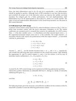
(a) Reference input r( t) and output x(t) (b) Control u(t) and disturbance w(t)
Fig. 6. Output response of the system (59) with controller (57) for a ramp reference input r(t),
where b
d
1
= 0andw(t)=0 (the reference model is a system of type 1)
(a) Reference input r( t) and output x(t) (b) Control u(t) and disturbance w(t)
Fig. 7. Output response of the system (59) with controller (57) for a step reference input r(t)
and a step disturbance w(t),whereb
d
1
= a
d
1
(the reference model is a system of type 2)
(a) Reference input r( t) and output x(t) (b) Control u(t) and disturbance w(t)
Fig. 8. Output response of the system (59) with controller (57) for a ramp reference input r(t),
where b
d
1
= a
d
1
and w(t)=0 (the reference model is a system of type 2)
Here e
k
:= r
k
− x
k

is the error of the reference input realization, r
k
being the samples of the
reference input r
(t), where the control transients e
k
→ 0 should meet the desired performance
129
PI/PID Control for Nonlinear Systems via Singular Perturbation Technique
PI/PID Control for Nonlinear Systems
via Singular Perturbation Technique 17
(a) Reference input r( t) and output x(t) (b) Control u(t) and disturbance w(t)
Fig. 9. Output response of the system (59) with controller (57) for a smooth reference input
r
(t) and a step disturbance w(t),whereb
d
1
= a
d
1
(the reference model is a system of type 2)
specifications given by (12).
By a
Z-transform of (12) preceded by a ZOH, the desired pulse transfer function
H
d
xr
(z)=
z −1
z

Z

L
−1

1/T
s(s + 1/T)





t=kT
s

=
1 −e
−T
s
/T
z −e
−T
s
/T
(62)
follows. Hence, from (62), the desired stable difference equation
x
k
= x
k−1

+ T
s
a(T
s
)[r
k−1
− x
k−1
] (63)
results, where
a
(T
s
)=
1 −e
−T
s
/T
T
s
, lim
T
s
→0
a(T
s
)=
1
T
,

and the output response of (63) corresponds to the assigned output transient performance
indices.
Let us rewrite, for short, the desired difference equation (63) as
x
k
= F(x
k−1
, r
k−1
), (64)
where we have r
k
= x
k
at the equilibrium of (64) for r
k
= const, ∀ k.Denote
e
F
k
:= F(x
k−1
, r
k−1
) − x
k
, (65)
where e
F
k

is the realization error of the desired dynamics assigned by (64). Accordingly, if for
all k
= 0, 1, . . . the condition
e
F
k
= 0 (66)
holds, then the desired behavior of x
k
with the prescribed dynamics of (64) is fulfilled. The
expression (66) is the insensitivity condition for the output transient performance with respect
to the external disturbances and varying parameters of the plant model given by (60). In
other words, the control design problem (61) has been reformulated as the requirement (66).
130
Advances in PID Control
18 Will-be-set-by-IN-TECH
The insensitivity condition given by (66) is the discrete-time counterpart of (15) which was
introduced for the continuous-time system (9).
7.2 Discrete-time counterpart of PI controller
Let us consider the following control law:
u
k
= u
k−1
+ λ
0
[F(x
k−1
, r
k−1

) −x
k
], (67)
where λ
0
= T
−1
s
˜
λ and the reference model of the desired output behavior is given by (63). In
accordance with (63) and (65), the control law (67) can be rewritten as the difference equation
u
k
= u
k−1
+
˜
λ

a
(T
s
)[r
k−1
− x
k−1
] −
x
k
− x

k−1
T
s

. (68)
The control law (68) is the discrete-time counterpart of the conventional continuous-time PI
controller given by (18).
7.3 Two-time-scale motion analysis
Denote f
k−1
= f (x
k−1
, w
k−1
) and g
k−1
= g(x
k−1
, w
k−1
) in the expression (60). Hence, the
closed-loop system equations have the following form:
x
k
= x
k−1
+ T
s
[ f
k−1

+ g
k−1
u
k−1
], (69)
u
k
= u
k−1
+
˜
λ

a
(T
s
)[r
k−1
−x
k−1
]−
x
k
−x
k−1
T
s

. (70)
Substitution of (69) into (70) yields

x
k
= x
k−1
+ T
s
[ f
k−1
+ g
k−1
u
k−1
], (71)
u
k
=[1−
˜
λg
k−1
]u
k−1
+
˜
λ
{
a(T
s
)[r
k−1
−x

k−1
]−f
k−1
}
. (72)
The sampling period T
s
can be treated as a small parameter, then the closed-loop system
equations (71)–(72) have the standard singular perturbation form given by (5)–(6). First, the
stability and the rate of the transients of u
k
in (71)–(72) depend on the controller parameter
˜
λ. Second, note that x
k
− x
k−1
→ 0asT
s
→ 0. Hence, we have a slow rate of the transients
of x
k
as T
s
→ 0. Thus, if T
s
is sufficiently small, the two-time-scale transients are artificially
induced in the closed-loop system (71)–(72), where the FMS is governed by
u
k

=[1 −
˜
λg
k−1
]u
k−1
+
˜
λ
{
a(T
s
)[r
k−1
− x
k−1
] − f
k−1
}
(73)
and x
k
= x
k−1
, i.e., x
k
= const (hence, x
k
is the frozen variable) during the transients in the
FMS (73).

Let g
= g
k
∀ k. From (73), the FMS characteristic polynomial
z
−1 +
˜
λg (74)
results, where its root lies inside the unit disk (hence, the FMS is stable) if 0
<
˜
λ
< 2/g.
To ensure stability and fastest transient processes of u
k
, let us take the controller parameter
131
PI/PID Control for Nonlinear Systems via Singular Perturbation Technique
PI/PID Control for Nonlinear Systems
via Singular Perturbation Technique 19
˜
λ
= 1/g, then the root of (74) is placed at the origin. Hence, the deadbeat response of the FMS
(73) is provided. We may take T
s
≤ T/η,whereη ≥ 10.
Third, assume that the FMS (73) is stable and consider its steady state (quasi-steady state), i.e.,
u
k
−u

k−1
= 0. (75)
Then, from (73) and (75), we get u
k
= u
id
k
,where
u
id
k
= g
−1
{
a(T
s
)[r
k−1
− x
k−1
] − f
k−1
}
. (76)
Substitution of (75) and (76) into (71) yields the SMS of (71)–(72), which is the same as
the desired difference equation (63) in spite of unknown external disturbances and varying
parameters of (60) and by that the desired behavior of x
k
is provided.
8. Sampled-data nonlinear system of the 2-nd order

8.1 Approximate model
The above approach to approximate model derivation can also be used for nonlinear system
of the 2-nd order, which is preceded by ZOH with high sampling rate. For instance, let us
consider the nonlinear system given by (43)
x
(2)
= f (X, w)+g(X, w)u, y = x,
whichisprecededbyZOH,wherey
∈ R
1
is the output, available for measurement; u ∈ R
1
is
the control; w is the external disturbance, unavailable for measurement; X
= {x, x
(1)
}
T
is the
state vector.
We can obtain the state-space equations of (43) given by
˙
x
1
= x
2
,
˙
x
2

= f (·)+g(·)u,
y
= x
1
.
Let us introduce the new time scale t
0
= t/T
s
. We obtain
d
dt
0
x
1
= T
s
x
2
,
d
dt
0
x
2
= T
s
{f (·)+g( ·)u}, (77)
y
= x

1
,
where dX/dt
0
→ 0asT
s
→ 0. From (77) it follows that
d
2
y
dt
2
0
= T
2
s
{f (·)+g (·)u}. (78)
132
Advances in PID Control
20 Will-be-set-by-IN-TECH
Assume that the sampling period T
s
is sufficiently small such that the conditions X(t)=const,
g
(X , w)=const hold for kT
s
≤ t < (k + 1)T
s
. Then, by taking the Z-transform of (78), we get
y

(z)=
E
2
(z)
2!(z − 1)
2
T
2
s
{
f (z)+{gu}(z)
}
, (79)
where
E
2
(z)=z + 1. Denote E
2
(z)=
2,1
z + 
2,2
and z
2
− a
2,1
z − a
2,2
=(z −1)
2

,where

2,1
= 
2,2
= 1, a
2,1
= 2, and a
2,2
= −1. From (79) we get the difference equation
y
k
=
2
∑
j=1
a
2,j
y
k−j
+ T
2
s
2
∑
j=1

2,j
2!


f
k−j
+ g
k−j
u
k−j

(80)
given that the high sampling rate takes place, where g
k
= g(X(t), w(t))
|
t=kT
s
, f
k
=
f (X(t), w(t))
|
t=kT
s
,and
y
k
−y
k−j
→ 0, ∀ j = 1, 2 as T
s
→ 0. (81)
8.2 Reference equation and insensitivity condition

Denote e
k
:= r
k
−y
k
is the error of the reference input realization, where r
k
being the reference
input. Our objective is to design a control system having
lim
k→∞
e
k
= 0. (82)
Moreover, the control transients e
k
→ 0 should have desired performance indices such as
overshoot, settling time, and system type. These transients of y
k
should not depend on the
external disturbances and varying parameters of the nonlinear system (43).
Let us consider the continuous-time reference model for the desired behavior of the output
y
(t)=x(t) in the form given by (45), which can be rewritten as
y
(s)=G
d
(s)r(s),
where the parameters of the 2nd-order stable continuous-time transfer function G

d
(s) are
selected based on the required output transient performance indices and such that
G
d
(s)



s=0
= 1.
By a
Z-transform of G
d
(s) preceded by a ZOH, the desired pulse transfer function
H
d
yr
(z)=
z −1
z
Z

L
−1

G
d
yr
(s)

s






t=kT
s

=
B
d
(z)
A
d
(z)
(83)
can be found, where
H
d
yr
(z)



z=1
= 1.
133
PI/PID Control for Nonlinear Systems via Singular Perturbation Technique

PI/PID Control for Nonlinear Systems
via Singular Perturbation Technique 21
Hence, from (83), the desired stable difference equation
y
k
=
2
∑
j=1
a
d
j
y
k−j
+
2
∑
j=1
b
d
j
r
k−j
(84)
results, where
1
−
2
∑
j=1

a
d
j
=
2
∑
j=1
b
d
j
,
2
∑
j=1
b
d
j
= 0,
and the parameters of (84) correspond to the assigned output transient performance indices.
Let us rewrite, for short, the desired difference equation (84) as
y
k
= F(Y
k
, R
k
), (85)
where Y
k
= {y

k−2
, y
k−1
}
T
, R
k
= {r
k−2
, r
k−1
}
T
,andr
k
= y
k
at the equilibrium of (85) for
r
k
= const, ∀ k.Bydefinition,putF
k
= F(Y
k
, R
k
) and denote
e
F
k

:= F
k
−y
k
, (86)
where e
F
k
is the realization error of the desired dynamics assigned by (85). Accordingly, if for
all k
= 0, 1, . . . the condition
e
F
k
= 0 (87)
holds, then the desired behavior of y
k
with the prescribed dynamics of (85) is fulfilled. The
expression (87) is the insensitivity condition for the output transients with respect to the
external disturbances and varying parameters of the plant model (80). In other words, the
control design problem (82) has been reformulated as the requirement (87). The insensitivity
condition (87) is the discrete-time counterpart of the condition e
F
= 0 for the continuous-time
system (43).
8.3 Discrete-time counterpart of PI DF controller
In order to fulfill (87), let us construct the control law as the difference equation
u
k
=

q ≥2
∑
j=1
d
j
u
k−j
+ λ
0
[F
k
−y
k
], (88)
where
d
1
+ d
2
+ ···+ d
q
= 1, and λ
0
= 0. (89)
From (89) it follows that the equilibrium of (88) corresponds to the insensitivity condition
(87). In accordance with (84) and (86), the control law (88) can be rewritten as the difference
134
Advances in PID Control
22 Will-be-set-by-IN-TECH
equation

u
k
=
q ≥2
∑
j=1
d
j
u
k−j
+ λ
0
⎧
⎨
⎩
−y
k
+
2
∑
j=1
a
d
j
y
k−j
+
2
∑
j=1

b
d
j
r
k−j
⎫
⎬
⎭
. (90)
The control law (90) is the discrete-time counterpart of the continuous-time PIDF controller
(50). In particular, if q
= 2, then (90) can be rewritten in the following state-space form:
¯
u
1,k
=
¯
u
2,k−1
+ d
1
¯
u
1,k−1
+ λ
0
[a
d
1
−d

1
]y
k−1
+ λ
0
b
d
1
r
k−1
,
¯
u
2,k
= d
2
¯
u
1,k−1
+ λ
0
[a
d
2
−d
2
]y
k−1
+ λ
0

b
d
2
r
k−1
, (91)
u
k
=
¯
u
1,k
−λ
0
y
k
.
Then, from (91), we get the block diagram of the controller as shown in Fig. 10.
Fig. 10. Block diagram of the control law (90), where q = 2, represented in the form (91)
8.4 Two-time-scale m otion analysis
The closed-loop system equations have the following form:
y
k
=
2
∑
j=1
a
2,j
y

k−j
+ T
2
s
2
∑
j=1

2,j
2!

f
k−j
+ g
k−j
u
k−j

, (92)
u
k
=
q ≥2
∑
j=1
d
j
u
k−j
+ λ

0
[F
k
−y
k
]. (93)
Substitution of (92) into (93) yields
y
k
=
2
∑
j=1
a
2,j
y
k−j
+ T
2
s
2
∑
j=1

2,j
2!

f
k−j
+ g

k−j
u
k−j

, (94)
u
k
=
q >2
∑
j=n+1
d
j
u
k−j
+
2
∑
j=1
[d
j
−λ
0
T
2
s

2,j
2!
g

k−j
]u
k−j
+λ
0
⎧
⎨
⎩
F
k
−
2
∑
j=1

a
2,j
y
k−j
−T
2
s

2,j
2!
f
k−j

⎫
⎬

⎭
.(95)
First, note that the rate of the transients of u
k
in (94)–(95) depends on the controller parameters
λ
0
, d
1
, ,d
q
. At the same time, in accordance with (81), we have a slow rate of the transients
135
PI/PID Control for Nonlinear Systems via Singular Perturbation Technique
PI/PID Control for Nonlinear Systems
via Singular Perturbation Technique 23
of y
k
, because the sampling period T
s
is sufficiently small one. Therefore, by choosing the
controller parameters it is possible to induce two-time scale transients in the closed-loop
system (94)–(95), where the rate of the transients of y
k
is much smaller than that of u
k
. Then, as
an asymptotic limit, from the closed-loop system equations (94)–(95) it follows that the FMS
is governed by
u

k
=
q >2
∑
j=3
d
j
u
k−j
+
2
∑
j=1
[d
j
−λ
0
T
2
s

2,j
2!
g
k−j
]u
k−j
+λ
0
⎧

⎨
⎩
F
k
−
2
∑
j=1

a
2,j
y
k−j
−T
2
s

2,j
2!
f
k−j

⎫
⎬
⎭
, (96)
where y
k
−y
k−j

≈ 0, ∀ 1, ,q, i.e., y
k
= const during the transients in the system (96).
Second, assume that the FMS (96) is exponentially stable (that means that the unique
equilibrium point of (96) is exponentially stable), and g
k
− g
k−j
→ 0, ∀ j = 1, 2, . . . , q as
T
s
→ 0. Then, consider steady state (or more exactly quasi-steady state) of (96), i.e.,
u
k
−u
k−j
= 0, ∀ j = 1, ,q. (97)
Then, from (89), (96), and (97) we get u
k
= u
id
k
,where
u
id
k
=[T
2
s
g

k
]
−1
⎧
⎨
⎩
F
k
−
2
∑
j=1

a
2,j
y
k−j
+ T
2
s

2,j
2!
f
k−j

⎫
⎬
⎭
. (98)

The discrete-time control function u
id
k
given by (98) corresponds to the insensitivity condition
(87), that is, u
id
k
is the discrete-time counterpart of the nonlinear inverse dynamics solution
(46). Substitution of (97) into (94)–(95) yields the SMS of (94)–(95), which is the same as the
desired difference equation (85) and by that the desired behavior of y
k
is provided.
8.5 Selection of discrete-time controller parameters
Let, the sake of simplicity, q = 2,
¯
g = g
k
= const ∀ k, and take
λ
0
= {T
2
s
¯
g
}
−1
, d
j
=


2,j
2!
,
∀ i = 1, 2. (99)
Then all roots of the characteristic polynomial of the FMS (96) are placed at the origin. Hence,
the deadbeat response of the FMS (96) is provided. This, along with assumption that the
sampling period T
s
is sufficiently small, justifies two-time-scale separation between the fast
and slow motions. So, if the degree of time-scale separation between fast and slow motions
in the closed-loop system (94)–(95) is sufficiently large and the FMS transients are stable, then
after the fast transients have vanished the behavior of y
k
tends to the solution of the reference
equation given by (85). Accordingly, the controlled output transient process meets the desired
performance specifications. The deadbeat response of the FMS (96) has a finite settling time
given by t
s,FMS
= 2T
s
when q = 2. Then the relationship
T
s
≤
t
s,SMS
2 η
(100)
136

Advances in PID Control
24 Will-be-set-by-IN-TECH
may be used to estimate the sampling period in accordance with the required degree of
time-scale separation between the fast and slow modes in the closed-loop system. Here t
s,SMS
is the settling time of the SMS and η is the degree of time-scale separation, η ≥ 10.
The advantage of the presented above method is that knowledge of the high-frequency gain
g suffices for controller design; knowledge of external disturbances and other parameters of
the system is not needed. Note that variation of the parameter g is possible within the domain
where the FMS (96) is stable and the fast and slow motion separation is maintained.
8.6 Example 3
Let us consider the system (59). Assume that the specified region of x(t) is given by x(t) ∈
[−
2, 2]. Hence, the range of high-frequency gain variations has the following bounds g(x) ∈
[
2, 6].WehavethatE
2
(z)=z + 1. Let the desired output behavior is described by the reference
equation (45) where a
d
1
= 2. Therefore, from (45), the desired transfer function
G
d
(s)=
b
d
1
Ts + 1
T

2
s
2
+ a
d
1
Ts + 1
=
b
d
1
Ts + 1
T
2
(s +
¯
α
)
2
(101)
results, where
¯
α
= 1/T. The pulse transfer function H
d
(z) of a series connection of a
zero-order hold and the system of (101) is the function given by
H
d
(z)=

¯
b
d
1
z +
¯
b
d
2
z
2
−
¯
a
d
1
z −
¯
a
d
2
, (102)
where
¯
a
d
1
= 2d,
¯
a

d
2
= −d
2
,
¯
b
d
1
= T
−2
[1 − d +(b
d
1
T −
¯
α
)dT
s
],and
¯
b
d
2
= T
−2
d[d −1 +(
¯
α
−

b
d
1
T)T
s
]. Take, for simplicity, q = 2. Hence, in accordance with (90) and (99), the discrete-time
controller has been obtained
u
k
= d
1
u
k−1
+ d
2
u
k−2
+[T
2
s
¯
g
]
−1
{−y
k
+
¯
a
d

1
y
k−1
+
¯
a
d
2
y
k−2
+
¯
b
d
1
r
k−1
+
¯
b
d
2
r
k−2
}, (103)
where d
1
= d
2
= 0.5. The controller given by (103) is the discrete-time counterpart of PID

controller (48). Let the sampling period T
s
is so small that the degree of time-scale separation
between fast and slow motions in the closed-loop system is large enough, then g
k
= g
k−1
=
g
k−2
, ∀ k. From (96) and (99), the FMS characteristic equation
z
2
+ 0.5

g
¯
g
−1

z + 0.5

g
¯
g
−1

= 0 (104)
results, where the parameter g is treated as a constant value during the transients in the FMS.
Take

¯
g
= 4, then it can be easily verified, that max{|z
1
|, |z
2
|} ≤ 0.6404 for all g ∈ [2, 6],where
z
1
and z
2
are the roots of (104). Hence, the stability of the FMS is maintained for all g ∈ [2, 6].
Let T
= 0.3 s. and η = 10. Take T
s
= T/η = 0.03 s. The simulation results for the output of
the system (59) controlled by the algorithm (103) are displayed in Figs. 11–15, where the initial
conditions are zero. Note, the simulation results shown in Figs. 11–15 approach ones shown
in Figs. 5–9 when T
s
becomes smaller.
137
PI/PID Control for Nonlinear Systems via Singular Perturbation Technique
PI/PID Control for Nonlinear Systems
via Singular Perturbation Technique 25
(a) Reference input r( t) and output x(t) (b) Control u(t) and disturbance w(t)
Fig. 11. Output response of the system (59) with controller (103) for a step reference input
r
(t) and a step disturbance w(t),whereb
d

1
= 0 (the reference model is a system of type 1)
(a) Reference input r( t) and output x(t) (b) Control u(t) and disturbance w(t)
Fig. 12. Output response of the system (59) with controller (103) for a ramp reference input
r
(t),whereb
d
1
= 0andw(t)=0 (the reference model is a system of type 1)
(a) Reference input r( t) and output x(t) (b) Control u(t) and disturbance w(t)
Fig. 13. Output response of the system (59) with controller (103) for a step reference input
r
(t) and a step disturbance w(t),whereb
d
1
= a
d
1
(the reference model is a system of type 2)
138
Advances in PID Control
26 Will-be-set-by-IN-TECH
(a) Reference input r( t) and output x(t) (b) Control u(t) and disturbance w(t)
Fig. 14. Output response of the system (59) with controller (103) for a ramp reference input
r
(t),whereb
d
1
= a
d

1
and w(t)=0 (the reference model is a system of type 2)
(a) Reference input r( t) and output x(t) (b) Control u(t) and disturbance w(t)
Fig. 15. Output response of the system (59) with controller (103) for a smooth reference input
r
(t) and a step disturbance w(t),whereb
d
1
= a
d
1
(the reference model is a system of type 2)
9. Conclusion
In accordance with the presented above approach the fast motions occur in the closed-loop
system such that after fast ending of the fast-motion transients, the behavior of the overall
singularly perturbed closed-loop system approaches that of the SMS, which is the same as
the reference model. The desired dynamics realization accuracy and an acceptable level of
disturbance rejection can be provided by increase of time-scale separation degree between
slow and fast motions in the closed-loop system. However, it should be emphasized that the
time-scale separation degree is bounded above in practice due to the presence of unmodeled
dynamics or time delay in feedback loop. So, the effect of unmodeled dynamics and
time delay on FMS transients stability should be taken in to account in order to proper
selection of controller parameters (Yurkevich, 2004). This effect puts the main restriction
on the practical implementation of the discussed control design methodology via singular
perturbation technique. The presented design methodology may be used for a broad class
of nonlinear time-varying systems, where the main advantage is the unified approach to
continuous as well as digital control system design that allows to guarantee the desired output
transient performances in the presence of plant parameter variations and unknown external
139
PI/PID Control for Nonlinear Systems via Singular Perturbation Technique

PI/PID Control for Nonlinear Systems
via Singular Perturbation Technique 27
disturbances. The other advantage, caused by two-time-scale technique for closed-loop
system analysis, is that analytical expressions for parameters of PI, PID, or PID controller with
additional lowpass filtering for nonlinear systems can be found, where controller parameters
depend explicitly on the specifications of the desired output behavior. The presented design
methodology may be useful for real-time control system design under uncertainties and
illustrative examples can be found in (Czyba & Błachuta, 2003; Khorasani et al., 2005).
10. References
Åström, K.J. & Hägglund, T. (1995). PID controllers: Theory, Design, and Tuning, Research
Triangle Park, NC: Instrum. Soc. Amer., ISBN 1-55617-516-7.
Błachuta, M.J.; Yurkevich, V.D. & Wojciechowski, K. (1997). Design of analog and digital
aircraft flight controllers based on dynamic contraction method, Proc. of the AIAA
Guidance, Navigation and Control Conference, 97’GN&C,NewOrleans,LA,USA,Part3,
pp. 1719–1729.
Błachuta, M.J.; Yurkevich, V.D. & Wojciechowski, K. (1999). Robust quasi NID aircraft 3D
flight control under sensor noise, Int. J. Kybernetika, Vol. 35, No. 5, pp. 637–650, ISSN
0023-5954.
Boychuk, L. M. (1966). An inverse method of the structural synthesis of automatic control
nonlinear systems Automation, Kiev: Naukova Dumka, No. 6, pp. 7–10.
Czyba, R. & Błachuta, M.J. (2003). Robust longitudinal flight control design: dynamic
contraction method Proc. of American Control Conf,Denver,Colorado,USA,
pp. 1020–1025, ISBN 0-7803-7896-2.
Hoppensteadt, F.C. (1966). Singular perturbations on the infinite time interval, Trans. of the
American Mathematical Society, Vol. 123, pp. 521–535.
Huang, J. & Rugh, W.J. (1990). On a nonlinear multivariable servomechanism problem,
Automatica, Vol. 26, pp. 963–972, ISSN 0005-1098.
Isidori, A. & Byrnes, C.I., (1990). Output regulation of nonlinear systems, IEEE Trans. Automat.
Contr., Vol. AC-35, No. 2, pp. 131–140, ISSN 0018-9286.
Khalil, H.K. (2000). Universal integral controllers for minimum-phase nonlinear systems, IEEE

Trans. Automat. Contr., Vol. AC-45 (No. 3), pp. 490–494, ISSN 0018-9286.
Khalil, H.K. (2002). Nonlinear Systems, 3rd ed., Upper Saddle River, N.J. : Prentice Hall, ISBN
0130673897.
Khorasani, K.; Gavriloiu, V. & Yurkevich, V. (2005). A novel dynamic control design scheme
for flexible-link manipulators, Proc. of IEEE Conference on Control Applications (CCA
2005), Toronto, Canada, 2005, pp. 595–600.
Klimushchev, A.I. & Krasovskii, N.N. (1962). Uniform asymptotic stability of systems of
differential equations with a small parameter in the derivative terms, J. Appl. Math.
Mech., Vol. 25, pp. 1011–1025.
Kokotovi´c, P.V.; O’Malley, R.E. & Sannuti, P. (1976). Singular perturbations and order
reduction in control – an overview, Automatica, Vol. 12, pp. 123–132, ISSN 0005-1098.
Kokotovi´c, P.V.; Khalil, H.K.; O’Reilly, J. & O’Malley, R.(1999). Singular perturbation methods in
control: analysis and design, Academic Press, ISBN 9780898714449.
Kokotovi´c, P.V. & Khalil, H.K. (1986). Singular perturbations in systems and control, IEEE Press,
ISBN 087942205X.
140
Advances in PID Control
28 Will-be-set-by-IN-TECH
Krutko, P.D. (1988). The principle of acceleration control in automated system design
problems, Sov. J. Comput. Syst. Sci. USA, Vol. 26, No. 4, pp. 47–57, ISSN 0882-4002.
Krutko, P.D. (1991). Optimization of control systems with respect to local functionals
characterizing the energy of motion Sov. Phys Dokl. USA, Vol. 36, No. 9, pp. 623–625,
ISSN 0038-5689.
Krutko, P.D. (1995). Optimization of multidimensional dynamic systems using the criterion of
minimum acceleration energy, Sov. J. Comput. Syst. Sci. USA, Vol. 33, No. 4, pp. 27–42,
ISSN 0882-4002.
Li, Y.; Ang, K.H. & Chong, G.C.Y. (2006). PID control system analysis and design, IEEE Contr.
Syst. Mag., Vol. 26, No. 1, pp. 32–41, ISSN 1066-033X.
Litkouhi, B. & Khalil, H. (1985). Multirate and composite control of two-time-scale
discrete-time systems, IEEE Trans. Automat. Contr., Vol. AC-30, No. 7, pp. 645–651,

ISSN 0018-9286.
Lun, J.Y.S.; Walker, M.W. & Paul, R.P.C. (1980). Resolved acceleration control of mechanical
manipulator IEEE Trans. Automat. Contr., Vol. AC-25, No. 3, pp. 468–474, ISSN
0018-9286.
Luo, G. & Saridis, G. (1985). L-Q design of PID controllers for robot arms, IEEE Journal of
Robotics and Automation, Vol. RA-1, No. 3, pp. 152–159, ISSN 0882-4967.
Mahmoud, N.A. & Khalil, H. (1996). Asymptotic regulation of minimum-phase nonlinear
systems using output feedback, IEEE Trans. Automat. Contr., Vol. AC-41, No. 10,
pp. 1402–1412, ISSN 0018-9286.
Meerov, M. V. (1965). Structural synthesis of high-accuracy automatic control systems,Pergamon
Press international series of monographs on automation and automatic control,
Vol. 6, Oxford, New York : Pergamon Press.
Morari, M. & Zafiriou, E. (1999). Robust Process Control, Englewood Cliffs, NJ. Prentice-Hall,
ISBN 0137819560.
Naidu, D.S. & Calise, A.J. (2001). Singular perturbations and time scales in guidance and
control of aerospace systems: a survey, Journal of Guidance, Control, and Dynamics,
Vol. 24, No. 6, pp. 1057-1078, ISSN 0731-5090.
Naidu, D.S. (2002). Singular perturbations and time scales in control theory and applications:
an overview, Dynamics of Continuous, Discrete & Impulsive Systems (DCDIS),SeriesB:
Applications & Algorithms, Vol. 9, No. 2, pp. 233-278.
O’Dwyer, A. (2003). Handbook of PI and PID Tuning Rules, London: Imperial College Press,
ISBN 1860946224.
Porter, W.A. (1970). Diagonalization and inverses for nonlinear systems, Int. J. of Control,
Vol. 11, No. 1, pp. 67–76, ISSN: 0020-7179.
Qu, Z.; Dorsey, J.F.; Zhang, X. & Dawson, D.M. (1991). Robust control of robots by the
computed torque method, Systems Control Lett., Vol. 16, pp.25–32, ISSN 0167-6911.
Saksena, V.R.; O’Reilly, J. & Kokotovi´c, P.V. (1984). Singular perturbations and time-scale
methods in control theory: survey 1976-1983, Automatica, Vol. 20, No. 3, pp. 273–293,
ISSN 0005-1098.
Slotine, J J. E. & Li, W. (1991). Applied nonlinear control, Prentice Hall, ISBN 0-13-040890-5.

Studenny, J. & Belanger, P.R. (1984). Robot manipulator control by acceleration feedback, Proc.
of 23th IEEE Conf. on Decision and Control, pp. 1070-1072, ISSN 0191-2216.
141
PI/PID Control for Nonlinear Systems via Singular Perturbation Technique
PI/PID Control for Nonlinear Systems
via Singular Perturbation Technique 29
Studenny, J. & Belanger, P.R. (1986). Robot manipulator control by acceleration feedback:
stability, design and performance issues, Proc. of 25th IEEE Conf. on Decision and
Control, pp. 80–85, ISSN 0191-2216.
Tikhonov, A.N. (1948). On the dependence of the solutions of differential equations on a small
parameter, Mathematical Sb., Moscow, Vol. 22, pp. 193–204.
Tikhonov, A.N. (1952). Systems of differential equations containing a small parameter
multiplying the derivative, Mathematical Sb., Moscow, 1952, Vol. 31, No. 3,
pp. 575–586.
Utkin, V.I. (1992). Sliding Modes in Control and Optimization, Springer-Verlag, ISBN-10:
0387535160.
Young, K.D.; Kokotovi´c, P.V. & Utkin, V.I. (1977). A singular pertubation analysis of high-gain
feedback systems, IEEE Trans. Automat. Contr., Vol. AC-22, No. 3, pp. 931–938, ISSN
0018-9286.
Young, K.D. & Özgüner, Ü. (1999). Variable structure systems, sliding mode, and nonlinear control,
Series: Lecture notes in control and information science, Vol. 247, ISBN 1852331976,
London, New York: Springer.
Yurkevich, V.D. (1995). Decoupling of uncertain continuous systems: dynamic contraction
method, Proc. of 34th IEEE Conf. on Decision & Control, Vol. 1, pp. 196–201, ISBN
0780326857, New Orleans. Louisiana.
Yurkevich, V.D. (2004). Design of nonlinear control systems with the highest derivative in feedback,
World Scientific Publishing Co., ISBN 9812388990, Singapore.
Ziegel, J.G. & Nichols, N.B. (1942). Optimum settings for automatic controllers, Trans. ASME,
Vol. 64, No. 8, pp. 759-768.
142

Advances in PID Control


Advances in PID Control

144
slide table using an AC linear motor and the third one is a slide table using synchronous
piezoelectric device driver (Egashira, Y. et al., 2002; Kosaka, K. et al., 2006). By the first
experiments, it is evaluated using single-axis slide system comprised of full closed feedback
via point-to-point control response and tracking control response when load characteristics
of the control target change. By the second experiments, it is evaluated using a linear motor
driven slider system via tracking control at low-velocity, and the resolution of this system is
10nm. By the third experiments, it is evaluated a stepping motion and tracking motion using
a synchronous piezoelectric device driver. Then, we derive control algorithm with nonlinear
compensator and describe each experimental results.
2. Control method
In this section, we describe a P,PI/I-P+FF control method and propose the P,PI/I-P+FF
control method with nonlinear compensator. The control objective is to design a control
input to track a given position reference.
2.1 Conventional P,PI/I-P+FF control method
In general, P,PI/I-P control method is applied in many industrial applications. To achieve
high-speed positioning response, velocity feed-forward compensation (FF) is usually
applied. The FF compensation is effective in compensating it for a response delay of the
positioning. As for P,PI/I-P method, positioning and velocity control are comprised of
cascade control. When we do not make positioning, we can control velocity by inputting a
direct velocity reference. Fig. 1 shows a block diagram of P,PI/I-P+FF control method. In
this figure, a signal x
d
is position reference, a signal x is table position, a signal x


is table
velocity, a signal e
1
is position error, a signal e
2
is velocity error and a signal u is control
input which means torque command, respectively. Here, the differentiation uses backward
difference equation. K
p
is position loop gain, K
i
is velocity integral gain, K
v
is velocity loop
gain, α is velocity feed-forward gain, β is the change fixed number to change velocity PI
control method or velocity I-P control method. If β is 1, the velocity control is I-P control
method, else if β is 0, the velocity control is PI control method. K
f
is the torque conversion
fixed number. The symbol s is Laplace transfer operator, s means differentiator and 1/s
means integrator.


Fig. 1. Block diagram of P,PI/I-P+FF control method.
The control input u is given as follows

High-Speed and High-Precision Position Control Using a Nonlinear Compensator

145

()
21
1
i
vf p d
K
uKK e Ke x
s
βα



=+−+






(1)
2.2 Proposed control method
In this paper, we will design a PID+FF controller with a nonlinear compensator for high
accuracy and a fast response with small overshoot. Fig. 2 shows a block diagram of the
P,PI/I-P+FF control method with proposed compensator. The algorithm of the nonlinear
friction compensator will be given.

r
u
+
+

+
-
+
-
+
+
・
+
-
・
・
・
T
c
x
d
e
1
e
2
xx
r
x
x

Fig. 2. Block diagram of proposed control method.
The dynamic equation of positioning table can be modelled as follows

Jx Dx F u++=
 

(2)
where J is the inertia, D is the viscous friction coefficient, F is the constant disturbance force,
x is table position , x

is table velocity, and u is the control input. Let the error value be

1 d
exx=− (3)

21
p
d
eKex x
α
=−+

(4)
Taking the second time derivative of both sides for (4) and substituting it into (2), we have

12pd
xKe x e
α
=+−
   
(5)

12
()
pd
JKe x e Dx F u

α
+−++=
 
(6)

21
()
pd
Je u J K e x Dx F
α
=− + + + +

(7)
Now, we can define the new signal as

()
21
1
i
vpd
K
rK e Ke x
s
βα



=+− +







(8)
Taking the time derivative of both sides for (8) and multiplying J to both sides, we have

Advances in PID Control

146

()
()
()
22 1
12
1
12
1
1
vvi pvvd
v
p
dvi
pv v d
vv v vd
pv vi
Jr JK e JK K e J K K e JK x
K u JK e J x Dx F JK K e
JKKe JK x

Ku KDx KF JK x
JK K e JK K e
βαβ
α
βαβ
αβ
β
=+ − −
=−+ + +++
−−
=− + + + −
+−+
  





(9)

We define the augmented signal as

() ()
12
11
rd
p
i
xx Ke Ke
αβ β

=−+ −+
  
(10)
Then, (9) can be rewritten as

vvrv v
Jr K u JK x K Dx K F=− + + +

(11)
Now, we give the control input u as

f
c
uKrT=+
(12)
where T
c
will be given later. Substituting (12) into (11), we have

v
f
vc vr v v
Jr KKr KT JKx KDx KF=− − + + +

(13)
The control input u must be determined that the closed-loop system becomes stable.
Analysing the closed loop stability, we give the following positive definite function as

2
1

2
VJr=
(14)
Taking the time derivative of both sides for (14) and substituting (13), we have

()
2
v
f
vr c
VJrr KKr KrJx DxFT==− + ++−


(15)
To achieve a negative
V

, the following inequality must be satisfied

()
0
vr c
Kr Jx Dx F T++−≤
 
(16)
Then, if we design T
c
as follows

max max max

sgn( )( )
cr
TrJxDxF=++
 
(17)
where J
max
, D
max
and F
max
are maximum values which are predetermined and known, then
inequality (16) is satisfied. This sgn function of r is established by a sliding mode control
theory. Therefore, if the control input (12) and (17) is applied, then the closed loop system is
stable in meaning of Lyapunov stability theory. However, chattering phenomena may occur,
because (17) contains the sgn function of r. To avoid the chattering phenomena, we
introduce an approximated function of the sign function as follows

High-Speed and High-Precision Position Control Using a Nonlinear Compensator

147

max max max
()
r
r
ur J x D x F
r
δ
=+ + +

+
 
(18)
where δ is the chattering avoidance parameter. Consequently, if we select sufficiently large
values of J
max
, D
max
and F
max
in (18), then the time derivative of (14) is always negative and
the control objective is accomplished. The P,PI/I-P+FF control method with nonlinear
compensator was derived.
3. Experimental results
In this section, we evaluated positioning responses and tracking responses by three kinds of
single-axis slide system experimentally. The first experimental system is two slider tables
that consists of an AC servo motor, a coupling and a ball-screw, and the second one is a
slide table using an AC linear motor and the third one is a slide table using synchronous
piezoelectric device driver.
3.1 A table drive system using AC servo motor with a coupling and a ball-screw
The first experiment system is two slider tables comprised of an AC servo motor, a coupling
and a ball-screw.
3.1.1 Experimental system
Fig. 3 shows the experimental setup which consists of the following parts. The control
system was implemented using a Pentium IV PC with a D/A converter board and a counter
board. The control input was calculated by the controller, and its value was translated into a
voltage input for the current amplifier through the D/A board. The positions of the
positioning table were measured by a position sensor with a resolution of 50 nm. The
sensor's signal was provided as a full-closed feedback signal. The sampling period was 0.25
ms. The table with 5 kg weight was mounted on a driving rail. The total inertia of the

moving part of the positioning table was approximately 1.128e-4 kgm
2
. The table was
supported by a rolling guide through the coupling that was connected with the motor, and
the table was driven by an AC servo motor (SGMAS-02ACA21,Yaskawa Electric. Co., Ltd), a
ball-screw lead of 20 mm (KR4620A+540L, THK Co., Ltd). The control parameters were set
to K
p
=75/s, K
v
=377 rad/s, K
i
=250 rad/s, α=0.55 or 0.60, β=1 and δ=5. The value of J
max
, D
max

and F
max
were selected as five times of J, D, F of the slide table (there is not a weight) which
measured beforehand, respectively.


Fig. 3. Experimental system of single axis slider.
Next, the results of positioning responses and tracking responses are shown.

Advances in PID Control

148
3.1.2 Experimental results

To evaluate our proposed method, we carried out three kinds of experiments. In the first
type experiment, it is evaluated that the case of positioning responses when the
acceleration/deceleration changes. In the second type of experiment, it is evaluated by the
case of positioning responses when the load changes. In the third type of experiment, it is
evaluated that the case of tracking responses when the load changes. Fig. 4 shows the
experimental table positioning results with the 5 kg-weight in which the positioning
reference acceleration/deceleration was changed. The acceleration/deceleration of the first
(left side) positioning reference is ±1.0 G, the second is ±1.5 G, the third is ±2.0 G, and the
fourth (right side) is ±3.0 G. In this figure, signal
① was the position reference x
d
(right side
vertical axis), signal
② was the position error (left side vertical axis) using the conventional
control method in which the feed-forward gain was set to 0.55, signal
③ was the position
error using the conventional control method in which feed-forward gain was set to 0.60, and
signal
④ was the position error using the proposed control method in which feed-forward
gain was set to 0.55. Fig. 5a shows an expanded graph at 1.0 G and Fig. 5b shows at 3.0 G. In
the case of an acceleration/deceleration of 1.0 G, all responses showed approximately the
same positioning control performance. However, in the case of an acceleration/deceleration
3.0 G, it is clearly found that there was undesired motion in the form of windup and
overshoot using the conventional control methods. On the other hand, there was no windup
or overshoot using the proposed control method.


Fig. 4. Position reference and table error.
These results demonstrated the effectiveness of the proposed control method. Generally, it
may be said that the acceleration 3.0 G in this experiment is very large because acceleration

is used in less than 2.0 G at the ball screw drive table. Fig. 6 shows a torque reference with
the conventional control method, and Fig. 7 shows a torque reference (signal
①) and
compensated torque T
c
(signal ②) with the proposed control method. The rate-torque of the
motor is 0.637 Nm, and in both figures, the maximum torque is about 150 % of the rate-
torque and is the same value in the conventional method and the proposed method. We
found that if a nonlinear compensated torque T
c
was very smoothly made, a chattering
phenomenon would probably not occur, and we could get a smooth response without any
vibration. Fig. 8 shows the response when δ changes in equation (18). In this figure, signal
① is the position reference with an acceleration/deceleration of 3.0 G, ②, ③, and ④ are