Electric Vehicles Modelling and Simulations Part 10 ppt

Mathematical Modelling and Simulation of a PWM Inverter Controlled Brushless
Motor Drive System from Physical Principles for Electric Vehicle Propulsion Applications

259


{ ( ) ( )}
()

{ ( ) ( )}
sca tri
sa
sca tri
Vvtvt
vt
Vvtvt






(LI)
with modulated pulse duration

2
{ ( ) }
(1 ) {| | 1}
0 { ( ) }
s
scad

T
ff
ca d
TvtA
mm
vt A












(LII)
for carrier amplitude
A
d
and modulation index (MI) m
f
given by

()
f
ca d
mvtA


(LIII)
The effect of the switch control voltage on the inverter base drive transistors T
A+
and T
A–
under ideal conditions, without delay is illustrated in Figures 13 and 14.
When blanking is introduced inverter switching is postponed until the capacitor voltages of
the complementary RC delay circuits, associated with power transistors T
A+
and T
A
–,
exceeds the threshold level setting
V
th
in the base drivers as shown in Figures 13 and 14 and
detailed in Figure 17. The magnitude of the delay

, typically 20µS, is given by

2
ln( ) 0.693 if 0
s
sth
V
th
VV
RC RC V





(LIV)
When phase-a power transistors T
A+
and T
A
–, are “OFF” during the blanking period
winding current conduction is maintained through free-wheeling protection diodes, as
shown in Figures 1 and 15, so that each transistor with its accompanying antiparallel diode
functions as a bilateral switch. The relationship between the states of the dc to ac converter
phase-a switch transistor pair, denoted by
S
A
(k) with k{0,1,2}, and the base drive voltages
&
la la
vv
in Figure 17 can be represented by

( ) 0 is "OFF"
(0)
() is "ON"
() is "ON"
(1)
() 0 is "OFF"
() 0 is "OFF"
(2)
() 0 is "OFF"

la th ba A
A
la th ba B A
la th ba B A
A
la th ba A
la th ba A
A
la th ba A
vV vt T
S
vV vtV T
vV vtV T
S
vV vt T
vV vt T
S
vV vt T






 



 


 



 

 



 

(LV)
with similar expressions
S
J
(k) and J{A,B,C} for the other two phases. The power
transistors in each leg of the inverter are thus alternately switched “ON” and “OFF”
according to the tristate expression (LV) with a brief blanking period separating these
switched transistor conduction states. The tristate operation of the power converter bridge
also determines the phase potential i/p of the stator winding as a result of the PWM
gating sequence applied to the basedrive in (LV). The corresponding converter voltages
applied between the stator phase winding input connection and ground, denoted by
v
ag
,
v
bg
, and v
cg

, are then given by

Electric Vehicles – Modelling and Simulations

260

Fig. 17. Transfer Function Block Diagram of a BLMD System (Guinee, 1999)
Pulse Width Modulator

-
+
Curre nt

Filter HDI
v
cj
3Current
Commutation
Filter HT
Velocity Controller
G
V

Shaft Velocity
Filtering
I
dj
Position Resolver
RC De lay
vlj=-Vs,vsj<0

,
vsj0
1+sRC
1
=-V
s,vsj0
v lj
,vsj0
1+sRC
1
Base Driv e
v
bj=VB,vljVth

=0 ,vljVth
Vth
Vth
v lj
=VB ,
=0 ,
v lj
v bj
v bj
Inverter State Sj (*)
S
j(0) {vbj=0,
S
j(1) {vbj>0,
S
j(2) {vbj=0,

>0}
=0}
=0}
v bj
v bj
v bj
vlj
v lj
vbj
v bj
Tr i a ng ul a r
Carrier
Inverter Output
v
jg=Ud
vjg=0
{
Sj(1)
S
j(2) & ijs<0
S
j(0)
S
j(2) & ijs>0
{
Stator Winding
Phase Voltage:
v
jg


v
js
+
Stator
Winding
Kt

l
+
Motor
Dynamics

e
-v
ej
Torque Constant
Bac k EMF Constant
Current Feedback
I
as
Ifj
+
-
Legend
Test Point
Phase j={a1,b2,c3}
Vtri
V
sj
=

V
s
, v
cj
 v
tri
-V
s
, v
cj
 v
tri



PWM
O/P
V
sj
V

r
K
c
1s

a
1s

b

Filter HFI
K
F
1  s

F
K
wi
Current
Demand
K
I
1s

d
sin p

r
 2( j 1)

3

1 s
Torque De mand
K
T
1s

T
K

p
 K
I
s

d
H
Vo

o
2
S
2


o
S 

o
2
V

V
js
 V
jg
 V
sg
V
sg


1
3
V
jg
j

1
r
s
sL
s
sin p

r
 2( j 1)

3


j
1
B
m
sJ
m
-
sin p

r

 2( j 1)

3


r

r
K
e
controller GI
Mathematical Modelling and Simulation of a PWM Inverter Controlled Brushless
Motor Drive System from Physical Principles for Electric Vehicle Propulsion Applications

261








(1) or 2 0
0 (0) or 2 0

(1) or 2 0
0 (0) or 2 0

(1) or 2 0

0 (0) or 2 0
dA A as
ag
AAas
dB B bs
bg
BBbs
dC C cs
cg
CCcs
US S() & i
v
SS() & i
US S() & i
v
SS() & i
US S() & i
v
SS() & i

























(LVI)
where current flow into a winding is assumed positive by convention. If the phase current
flow i
js
is positive in (LVI) during blanking when power transistors T
J+
and T
J-
are “OFF”, as
shown in Figure 15, then v
jg
= 0. If, however, i
js
is negative then v
jg
= U
d

while T
J+
and T
J-
are
blanked. The tristate operation of the inverter bridge also uniquely determines the phase
potential i/p v
jg
of the stator winding in (LVI) as a result of the PWM gating sequence
applied to the basedrive in (LV). The inverter o/p voltage v
ag
is shown in Figures 18 and 19
for the two cases of current flow direction in phase-a of the stator winding. The potential of
the stator winding neutral star point s, from equation (XXIII) with phase current summation

3
1
0
js as bs cs
j
iiii




(LVII)
is given by

1
3

()
s
g
a
g
b
g
c
g
v vvv (LVIII)
with resultant phase voltages

1
3
1
3
1
3
()(2 )
()(2 )
()(2 )
as a
g
s
g
a
g
b
g
c

g
bs b
g
s
g
b
g
a
g
c
g
cs c
g
s
g
c
g
a
g
b
g
vvv vvv
vvv vvv
vvv vvv
 
 
 
(LIX)

-0.1 0.1 0.3 0.5 0.7 0.9 1.1 1.3

-100
0
100
200
300
400
Stator Winding I/P Voltage Vag
Time (mS)
Phase a Current Flow Condition (Ias>0)
Ud
MI=0.72 Ad=6.9 Volts
Vm=5 Volts Fm=833Hz

-0.1 0.1 0.3 0.5 0.7 0.9 1.1 1.3
-100
0
100
200
300
400
Stator Winding I/P Voltage Vag
Time (mS)
Phase a Current Flow Condition (Ias<0)
Ud
MI=0.72 Ad=6.9 Volts
Vm=5 Volts Fm=833Hz

Fig. 18. Inverter o/p Voltage (i
as
>0) Fig. 19. Inverter o/p Voltage (i

as
<0)

Electric Vehicles – Modelling and Simulations

262
The complete three phase model of a typical high performance servo-drive system (Moog
GmbH, 1989; Guinee, 1999). incorporating equations (XXIII), (XXIV), (XLII), (IL), (L), (LV),
(LVI) and (LIX), used in software simulation for parameter identification purposes is
displayed in Figure 17.
3. Numerical simulation accuracy and experimental validation of BLMD
model
Since the BLMD model is partitioned into linear elements and non linear subsystems, owing to
the complexity and discrete temporal nature of the PWM control switching process, numerical
integration techniques have to be applied to obtain solutions to the differential electrodynamic
equations of motion. Numerical simulation of the continuous-time subsystems, with a transfer
function representation based on the Laplace transform, is achieved by means of model
difference equations with numerical solutions provided by the use of the backward Euler
integration rule (BEIR) (Franklin et al, 1980). In this instance continuous time derivatives are
approximated in discrete form using the Z Transform substitution operator
1
1
(1 )
T
SZ

 .
Since the BEIR maps the left half s-plane inside the unit circle in the z-plane these solutions are
stable. The choice of this implicit integration algorithm is based on its simplicity of
substitution, ease of manipulation with a small number of terms and reduced computation

effort in the overall complex BLMD model simulation. An alternative filter discretization
process based on Tustin’s bilinear method, or the trapezoidal integration rule with the
substitution operation
)1()1(
11
2

 ZZS
T
, can be implemented with negligible
observable differences at the small value of integration step size T actually chosen. The
application of the BEIR technique can be visualized for a first order system, as in the case of the
current control lag compensator G
I
which has a generalized transfer function (Guinee, 2003)

01
01
1()
() 1
()
a
b
ssVs
Ic
Is s s
Gs K K







  , (LX)
with continuous-time description given by



() ()
01 01
() ()
dV t dI t
dt dt
Vt K It
 
  (LXI)
Integrating (LXI) between the discrete time instants t
k
and t
k-1
with a fixed time step size T gives


11
1111110 0
() () () () () ()
kk
kk
tt
kkk k

tt
Vt K It Vt K It K I d V d

  


   

(LXII)
Applying the BEIR, with piecewise constant integrand backward approximations V(t
k
) and
I(t
k
) over the interval t
k
 t > t
k-1
yields the input-output difference equation





10 1 1 10 1 1
() ( ) () ( )
kk kk
Vt T Vt K TIt K It
   


    (LXIII)
This can be expressed in the Z domain, via the Z Transform, as the transfer function




1
1
1
01
01
1
1
1
01
01
1
()
()
1
T
T
Z
nnZ
VZ
IZ
ddZ
Z
Kk











 (LXIV)
Mathematical Modelling and Simulation of a PWM Inverter Controlled Brushless
Motor Drive System from Physical Principles for Electric Vehicle Propulsion Applications

263
which is equivalent to (LX) through the general BEIR substitution operator
1
1
(1 )
T
SZ

 .
The time evolution of each discretized linear subsystem proceeds according to the BEIR,
similar to (LXIII), as an integral part of the overall BLMD numerical simulation with a fixed
time step
T=t and input x(t) to output y(t) relationship given by

1
11
00

01
()
kk k
d
k
k
dd
y
nx nx y


  (LXV)
The choice of time step size is determined by the resolution accuracy of the PWM switching
instants required during simulation for delayed inverter trigger operation as explained in
section 3.1 below. The BLMD model program is organized into a sequence of software
function calls, representing the operation of the various subsystems.
3.1 PWM simulation with inverter delay
The choice of numerical integration step size t, for solution of the set of dynamic system
differential equations, is influenced by the PWM switching period
T
S
(≈200S) (Moog, 1989)
and the smallest BLMD time constant

d
(~28.6S) associated with the basedrive ‘lockout’
circuitry. Furthermore the precision with which the pulse edge transitions are resolved in
the three phase PWM o/p sequences as in (LI) with inverter blanking included, has a
significant effect on the accuracy of the inverter o/p waveforms. This is important in BLMD
simulation where model accuracy and fidelity are an issue in dynamical parameter

identification for optimal control. The effect of inaccuracy in pulse time simulation can be
reduced by choosing a sufficiently small fixed time step
∆t << T
s
, such as 0.5%T
S
or 5% of
the inverter dead time
 (≈20S) for example, to reflect overall BLMD model accuracy and
curtail computational effort in terms of time during lengthy simulation trial runs.
Furthermore this choice of step size also provides an uncertainty bound of +
t in the
evaluation of PWM switching instants during simulation in the absence of an iterative
search of the switch crossover time. This uncertainty can be reduced by an iterative search of
the PWM crossover time
t
*
within a fixed assigned time step size t during BLMD
simulation for which a width modulated pulse transition has been flagged as shown in
Figure 16. A variety of iterative search methods can be employed for this purpose with
varying degrees of computation runtime required and complexity. These include, for
example, successive application of the bisection method, regula falsi technique and the
Newton-Raphson approach (Press et al, 1990) where convergence difficulties can arise with
derivative calculations from noisy current control signals. The number of iterations
n
required for the bisection technique, with a fixed time step t, to reach an uncertainty  in
the pulse transition time estimate
t
X
, is given by the error criterion

(1)
2
n
t




(LXVI)
The estimate of the PWM switching time
t
*
obtained via the regula falsi method, from the
comparison of the triangular carrier ramp with the piecewise linear approximation of the
control signal
v
cj
as shown in Figure 16, is given by the iterative search value t
X
as (Guinee,
1998, 2003)

11
11
{( ) ( )}
1
{( ) ( )}{() ()}
tri k cj k
trik cjk trik cjk

vt vt t
k
v t vt v t vt
X
tt





 (LXVII)

Electric Vehicles – Modelling and Simulations

264
The adoption of a single iteration of the regula falsi method along with a small simulation
time step
t simplifies the search problem of the pulse edge transition with sufficient
accuracy without the expenditure of considerable computational effort for a modest gain in
accuracy by comparison with the other iterative methods available. An indication of the step
size required for accurate resolution of PWM inverter operation with delay can be obtained
from consideration of the anticipated signal ‘curvature’ due to (a) the signal bandwidth and
amplitude at the current controller o/p v
cj
in the magnitude comparison with the triangular
carrier shown in Figure 16 in the comparator modulator and (b) the rate of exponential
voltage ramp up to the base drive threshold V
th
, which controls the inverter dead time, in
the RC delay circuits shown in Figure 20.

The maximum harmonic o/p voltage from the high gain current compensator
G
I
is
determined by the carrier amplitude
A
d
at the onset of overmodulation (m
f
= 1) in PWM
inverter control with a frequency that is limited by the 3dB bandwidth

F
= 1/
F
(~3kHz in
Table I) of the smoothing filter
H
FI
in the current loop feedback path shown in Figure 17.
This may be represented in analytic form as

() sin( )
cj d F
vt A t


(LXVIII)

Vlj

Vlj
0 50 100 150 200 250
-25
-20
-15
-10
-5
0
5
10
Base_Drive Voltages Volts
Time (uS)
V
s
-Vs
C
R
Comparator
o/p V
sj
Base Drive
i/p V
lj
Base Drive
Threshold V
th
Base Drive Voltage Vlj
Complementary Base Drive Voltage V
lj



TJ+ ON
TJ- OFF
TJ+ OFF
TJ- ON

Iterative Step Size t
Basedrive
Time
tk-1 tktX
Threshold Vth
Basedrive
exponential V
lj
Piecewise Linear
Approximation
t**

Fig. 20. Delayed basedrive trigger signals Fig. 21. Basedrive Trigger Time Search
with a quadratic power series approximation about the mid interval point
ˆ
t
in t given by

ˆ
()
2
2!
ˆˆˆ ˆ
() () ()( ) ( )

cj
vt
cj cj cj
vt vt vttt tt



  
. (LXIX)
The accuracy with which the estimated width modulated pulse transition instants
t
X
are
determined can be gauged by comparing the deviation error of the actual intersection time
t
*

of the triangular carrier with the control signal v
cj
, due to its curvature, to that t
X
obtained
with the piecewise linear chord approximation of the signal in the regula-falsi method as
illustrated in Figure 16. The ‘curvature’ of the signal in (LXVIII) with time, determined
(Kreyszig, 1972) from

2
1
c
j

c
j
vv




, (LXX)
Mathematical Modelling and Simulation of a PWM Inverter Controlled Brushless
Motor Drive System from Physical Principles for Electric Vehicle Propulsion Applications

265
is given by its maximum value

2
max
c
j
dF
vA




(LXXI)
at the peak amplitude
A
d
of v
cj

(t) corresponding to the instant 2
F
t



 in Figure 16 at
which ( ) cos( ) 0
cj d F F
vt A t




. The peak deviation l
V
of the signal due to curvature from
the chord approximation through
t
k-1
in Figure 16 occurs at
ˆ
tt


with zero chord slope. The
peak deviation from the chord, through
1
(2)
k

ttt


 , is determined by the Taylor series
expansion in (LXIX) about
ˆ
tt


with




2
2
()
1
1
2! 2 2 2
() () 1
cj
F
vt
t
t
cj k cj d
vt vt A










 




(LXXII)
giving



2
1
22
() ( )
d
F
A
t
vcj cjk
lvtvt






 

. (LXXIII)
The worst case deviation error of the pulse transition time estimate t
X
from t


is determined
by the regula-falsi method at the point of intersection t
X
of the carrier ramp, which passes
through the signal coordinates [t

, v
cj
(t

)] in Figure 16, with the chord approximation to the
signal. The approximation error (t


- t
X
) is determined from the ramp, which has peak-to-
peak excursion 2A
d
over the half period T

S
/2, with slope m = 4A
d
/T
S
as









2
82
vs
F
lT
t
x
m
tt





(LXXIV)

Substitution of the set of relevant signal parameters
{, ,}
SdF
TAf , for a step size of 1s, with
values {200 , 6.9V, 3kHz}s

result in a negligible approximation error  relative to the step
size
t of 0.222% which verifies the suitably of the chosen step size for a linear search of the
PWM crossover time. The PWM resolution accuracy determines the moment that a
modulated pulse edge transition takes place with subsequent onset of inverter blanking,
using lockout circuitry, which substantially affects power transfer from the dc supply to the
prime mover. The next essential trigger event, that needs to be accurately resolved, is the
instant at which retarded firing of the inverter power transistors commences when the RC
delay growth voltage exceeds the basedrive threshold V
th
= 0 in Figure 20. The
complementary exponential trigger voltages

&
l
j
l
j
vv supplied to the basedrive circuitry, for
a modulator peak-to-peak o/p swing of 2V
S
, can be expressed as

(1 2 )

tRC
lj s
vV e


. (LXXV)
The basedrive turnon time t
**
is given by (LIV) as  (~19.82S), at the instant at which
()
l
j
th
vt V

 , for a time constant 
d
(~28.6S). Since delay circuit simulation is employed the
trigger instant t
X
has to be obtained using piecewise linear approximation of the exponential
growth waveform, within the flagged simulation interval as shown in Figure 21, and is given by

1
1
()
1
() ( )
lj k
lj k lj k

vt
xk
vt vt
tt t






(LXXVI)

Electric Vehicles – Modelling and Simulations

266
where
1kk
ttt
x
 and
**
1


kk
ttt

. Assume that t
**
occurs at the mid interval time

1
(2)
k
tt

 which thus provides an absolute point of reference for comparison with the
search estimate t
X
. The effect of basedrive signal ‘curvature’ on the trigger estimate t
X
can be
gauged by monitoring the relative contribution of the quadratic terms in the Taylor series
expansion about t
**
as

()
2
2!
() () ()( ) ( )
lj
vt
ll l
xxx
vt vt vt t t t t
jjj



 


  
(LXXVII)
with v
lj
(t**) = V
th
= 0. The differential error  in the crossover time estimate in (LXXVI) is
given by

2
22
3
1
1
2
( ) 4.37 10
t
RC
tt
RC RC
e
x
ee
tt t t




 





   


(LXXVIII)
and is practically zero for very small time steps which implies a negligible quadratic
contribution. Consequently the trigger time estimate obtained by linear approximation of
the basedrive voltage about the threshold is very accurate for the time step size chosen.
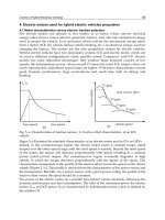
3.2 Motor dynamic testing and simulation
The steady state controlled torque versus output speed characteristic (Moog, 1988) for the
particular motor drive concerned is almost constant over a 4000 rpm speed range for a rated
continuous power o/p of 1.5kW. The corresponding dynamic transfer characteristic of o/p
motor torque 
e
versus input torque demand 
d
voltage is practically linear in the range (0,
10) volts. A fixed step signal 
d
i/p is chosen to provide persistent excitation, as a standard
control stimulus for dynamic system response testing, and in particular to gauge the
accuracy of the model simulation and parameter extraction process based on the feedback
current (FC) response i
fj
. This response has the transient features of a constant amplitude
swept frequency sinusoid, during the acceleration phase of the motor shaft, which are
beneficial for test purposes and BLMD model validation in system identification (SI). The

phase current feedback simulation can then be checked against experimental test results as
the observed target data, for example in phase-a, for both phase and frequency coherence in
model validation. Further model validation is provided by the accuracy with which high
frequency ripple in the unfiltered current feedback is replicated through BLMD simulation
when compared with experimental test data. Examination of the presence of dead time
related low frequency harmonics in the simulated current feedback is also used to gauge
BLMD model fidelity, through FFT spectral analysis, when compared with measurement
data. An input magnitude of 1volt is sufficient to guarantee linear operation and avoid
saturation (m
f
>1) of the PWM stage by the high gain current controller chosen here as the
optimizer module MCO 402B in Table 1. This input step size is also enough to slow down
the rate of shaft speed ramp up to allow adequate resolution of the frequency change in the
FC target data.
The intrinsic mechanical parameters of motor viscous friction B
m
and shaft inertia J
m
are
initially determined from experimental motor testing and cost surface simulations based on
the mean squared error (MSE) between the simulated and measured transient response data
for shaft velocity and current feedback. Two examples of known shaft load inertia J
L
are
Mathematical Modelling and Simulation of a PWM Inverter Controlled Brushless
Motor Drive System from Physical Principles for Electric Vehicle Propulsion Applications

267
then used in simulated response measurements as a check against BLMD test data for
further model accuracy and validation. These simulation results, which correspond to the

different inertial loads, are integrated into a parameter identification process, using MSE
cost surface simulation, based on a Fast Simulated Diffusion (FSD) optimization technique
for the purpose of motor drive shaft parameter extraction. The experimentally determined
parameter values listed in Table II for the BLMD model are used in all model simulations.
The back EMF or voltage constant K
e
was experimentally determined from an open circuit
(o/c) test with the motor configured as a generator driven over a range of speeds by an
identical shaft coupled BLMD system. The generator voltage characteristic V
g
is linear with
drive shaft speed 
m
as shown for the experimental data in Figure 22, according to (XXIV),
with slope K
e
derived from the fitted linear voltage relationship V
f
.
The transducer velocity ‘gain’ G
RDC
of the Resolver-to-Digital Converter (RDC) was
concurrently estimated along with K
e
from the slope of the fitted linear characteristic V
f

,
which in addition substantiates the converter linearity, to the speed voltage measurements
shown in Figure 23. This value along with the cascaded shaft velocity filter gain is given as

the cumulative gain H
vo
in Table II.

Torque Demand Filter
H
T

K
T
=1.0;

T
=222S
Voltages
U
d
=310 Volts; V
th
=0;
V
S

=10 Volts
Current Demand Filter
H
D
I

K

I
=1.0;

I
=100S
Constants K
wi
=6.8x10
-2
; K
e
= K
t
=0.3
Current Feedback Filter
H
FI

K
F
=5.0;

I
=47S
Winding
P =6; r
S
=0.75 Ohms;
L
S

=1.94mH
Basedrive Delay Circuit
RC =28.6S
Carrier f
S
=5kHz; A
d
=6.9 Volts;
Current Controller Type


High Gain: MCO 402B

Low Gain: MCO 422
K
C
=19.5;

a
=225s;

b

=1.5ms

Motor
Dynamics

J

m
=3 kg.cm
2
;

B
m
=2.14x10
-3
Nm.rad
-1
.sec
K
C
=5.0;

a
=223S;

b

=0.7mS
Shaft Velocity Filter H
V

H
vo
=13.5x10
-3
;

=
√2;

o
=2x10
3
rad.sec
-1

Inertial
Loads
J
MML
=9.06 kg.cm
2

(Medium Mass –MML)
* J
LML
=17.8 kg.cm
2
(Large Mass – LML)
*Returned Parameter Estimates:
2
ˆˆ
20.838 k
g
.cm
opt m LML
JJJ  ,

3-1
ˆ
1.959 10 Nm.Sec.Rad
opt
Bx


* Simulated FC Response Surface Estimates: J
opt
=20.877 kg.cm
2
,
B
o
pt
=1.921x10 Nm.Sec.Rad
-1

Table II. BLMD system parameters

Electric Vehicles – Modelling and Simulations

268
100 200 300 400
50
100
150
R
otor Shaft Angular Velocity


r
F
itted Voltage V
f
Generated voltage
V
g
Rads/sec
Open Circuit Voltage Test
V
O
L
T
S
Slope =0.315=
E
MF Constant
K
e

200 400 600
0
2
4
6
M
otor Shaft Velocity

r
0

Rads/sec
V
O
L
T
S
S
ha
f
t S
p
eed Volta
g
e Tes
t
Shaft Speed
V

F
itted Voltage
V
f

Slope
=
G
R
DC
=
1.16x10

-3

R
DC Voltage Gain

Fig. 22. Estimation of EMF constant K
e
Fig. 23. Estimation of RDC ‘gain’ G
RDC

The value of K
e
was subsequently used in a motor-generator electrical load test, at different
speeds as illustrated in Figure 24, to estimate the stator winding parameters L
s
and r
s
as a
cross check of the nominal catalogued (Moog, 1998) values. The difference
V between the
measured terminal voltage V
T
, across the load resistance R
L
, and the generated voltage V
G

using the fitted coefficient K
e
via (XXIV) is equated to the internal voltage drop of the

Thevenin equivalent circuit shown in Figure 24
with


||
GT L
VVVZI  
(LXXIX)
where

/
LTL
IVR

.

50 100 150
0
20
40
60
80
Generator Electrical Load Test
Rheostat Load R
L
=18.3

EMF Constant K
t
=0.315

Shaft Speed

r
Rads/sec
~
Z
I
R
L
V
T
V
G
I
L
0
V
O
L
T
S
Terminal Voltage V
T
Generator Voltage V
G

50 100 150
0
2
4

6
8
0
M
otor - Generator Electrical Load Test
Shaft Speed 
r
Rads/sec
Terminal Voltage V
T
Generated Voltage V
G
Differential Voltage

V = V
G
- V
T
Internal Voltage Drop V
I
=

Z
I

I
L
P
arameter Estimates
r

s
=0.724

;
L
s
=1.945mH
V
O
L
T
S

Fig. 24. Motor - generator load test Fig. 25. Winding parameter estimation
Mathematical Modelling and Simulation of a PWM Inverter Controlled Brushless
Motor Drive System from Physical Principles for Electric Vehicle Propulsion Applications

269
The quadratic polynomial expressed in terms of 
e
via the circuit parameters as

22
00

e
Zabw
, (LXXX)
for


e
= p
r
and constant coefficients a
0
 r
2
s
and b
0
 L
2
s
, is fitted to the derived data y =
(
V/I
L
)
2
. The quadratic fit shown in Figure 25 is based on the minimization of the MSE (E),
between the sampled y
k
and simulated Z
k
2
data, as

2
2
1

00
1
for
N
kk e
N
k
Eyabxx



 


(LXXXI)
with respect to a
0
and b
0
. The cost function minimisation results in the normal equations


22
2
222
0
T
kk
kk
T

k
k
x
y
NY X
xXX
b





(LXXXII)

2
1
00
kk
N
kk
aybx






(LXXXIII)
with parameter estimates
ˆ

1.945mH
s
L 
and
ˆ
0.724 ohms
s
r

that are very close to the
nominal values in Table II.
The motor shaft friction coefficient B
m
was obtained from the steady state current feedback
I
fa
in phase-a at various shaft speeds 
r
by means of the torque constant K
t
which is
numerically equal to the experimentally determined value of K
e
when proper units are used.
The active component of the steady state current feedback is considered in the calculation of
the dissipative friction torque by allowing for the effect of the machine impedance angle

Z

increase, given by





11
sjs
rs
sjs s
XI
p
L
z
rI r
Tan Tan




, (LXXXIV)
with motor shaft speed and zero load angle

T
in Figure 10. This is necessary in electronic
commutated motor drive systems, in which the current controlled applied phase voltage v
js

at zero load angle is derived from the current demand I
dj
in Figure 17, without the benefits

of adaptive current angle advancement (Meshkat, 1985) to counteract the torque reduction
effects of internal power factor angle illustrated in Figure 10. The derived friction torque,
from the adjusted measured current feedback I
fa
cos 
z
, is given by

 


33
22
cos cos
t
wi f
K
f
tas z
f
az
KK
KI I


 
(LXXXV)
via (XLV) for balanced 3-phase conditions where the current feedback factor K
wi
and filter

gain K
f
are considered in the estimation of the stator current flow I
js
. This is graphed in
Figure 26 for the measured FC test data I
fa
and equated to the steady state mechanical
friction torque via (IL) as

f
mr
B


 . (LXXXVI)

Electric Vehicles – Modelling and Simulations

270
100 200 300 400
0.5
1
Shaft Velocity

m
Rads/sec
Motor Testing for Shaft Friction
B
m

Estimation
Friction Torque

f
estimation
via FC
I
fa
Fitted estimate


f
Friction Coefficient Estimate

.B
m


2141 10
3
Nm.rad
-1

200 400
200
400
600
Rads/sec
Shaft Velocity


r
S
ha
f
t Friction
B
m
Estimation
f
rom Power Considerations
Mechanical Pow - Estim
n
P
m
Electrical pow - Estim
n
P
e
W
a
t
t
s

Fig. 26. Friction parameter estimation Fig. 27. Friction power estimation
The friction coefficient B
m
is obtained from a linear first order polynomial fit, displayed in
Figure 26, based on expression (LXXXVI) with estimate
3-1

ˆ
2.141 10 Nm.rad
m
B

 as in
Table II. Alternative confirmation of the accuracy of the damping factor estimate is obtained
from consideration of the electrical power transfer P
e
from the coupling field expressed in
(XLVII) and comparison with the resultant mechanical power dissipation P
m
associated with
dynamic friction via (XLVI). The continuous power supplied from the coupling field,
necessary to sustain motor rotation with frictional losses at various shaft speeds under
steady state conditions, is determined from the rms values of reaction EMF using the
measured estimate
ˆ
e
K from the o/c test and the experimental FC test data with lagging
power factor balanced over three phases as



ˆ
22
3cos
fa
er
wi f

I
K
ez
KK
P






. (LXXXVII)
The mechanical power dissipated as frictional heat is evaluated from (LXXVI) using the
measured estimate
ˆ
m
B as

2
ˆ
m
f
rmr
PB


  (LXXXVIII)
Both power estimates exhibit a high degree of correlation, with correlation coefficient


(Bulmer, 1979) of 99.5%, when plotted in Figure 27 which validates the derived damping
factor estimate
ˆ
m
B
.
3.3 Motor step response testing and simulation results
Synchronized initial conditions for BLMD testing, and resultant comparison with model
numerical simulation, are obtained by hand cranking the motor shaft to top dead centre of
the phase-a current commutation reference position while monitoring the phase generator
o/p waveforms before application of the torque demand step i/p. This is essential for
Mathematical Modelling and Simulation of a PWM Inverter Controlled Brushless
Motor Drive System from Physical Principles for Electric Vehicle Propulsion Applications

271
proper datum time referencing of all waveforms in the eventual comparison process, when
formulating a multiminima cost surface for minimization purposes using the least squares
error criterion, during parameter identification.

Torque
Demand

cos(pr-2(j-1)/3)
Gv
3

Current
Commutation
3


Current Command
Filtering
HDI
3Current
Controller
Idj
GI
+
-
3PWM
Modulator
Triangular
Carrier
Vtri
Vcj
3 Delay
Network
j
BDj
Tj+
Tj-
3BASE
DRIVE
Ijs

Filtering
HFI
Hall Effect
Device HED
3


Current Feedback
Phase Generator
ROM Table
Shaft Velocity
Filter Hv
Position
r
Velocity Feedback r

Velocity
V
d
Lss
3

Stator winding

HT Busbar Ud
3 PWM
INVERTER
rs
HT
R
C
j
Command
Filtering
Controller
Vsj

Vjg
Vbj
Vbj
PM Rotor
P pole Pairs
Shaft Inertia Jm
Friction
Bm
Shaft Position
Resolver
-
+
Ifj

r


Fig. 28. Network structure of a typical BLMD system
The actual drive system with network structure as shown in Figure 28 was tested at critical
internal nodes with multiplexed sampled data waveforms acquired at rates corresponding
to the different inertial loaded shaft conditions (J
L
) specified in Table III. The length of each
data record is fixed at 4095 sample points with a normalized duration of approximately 10
machine FC cycles for reference purposes during comparison with simulated motor
response for model validation and accuracy and also during system identification for
accurate extraction of drive motor model parameter estimates.

FC Target Data
No. of machine cycles

Acquisition rate T
No. of data points N
d

No Shaft Load (NSL)

~ 9.75
20
s
4095
Medium Inertial Load (MML)

~ 11.5
40
s
4095
Large Inertial Load (LML)
~ 10.5
49.6
s
4095
Simulation time step

Decimation Factor
1
s
20
1s
40

1s
50
Waveform Correlation Analysis for BLMD system without inertial shaft loads
Signal x Exp I
xa
Sim i
xa
Data Correlation Coefficient 
Current Feedback Fig. 29: I
fa
i
fa
0.985
Current Demand Fig. 30: I
da
i
da
0.993
Current Controller o/p Fig. 31: V
ca
v
ca
0.98
Motor Shaft Velocity
Fig. 32: V

r
v

r

0.98
Table III. Brushless Motor Drive Test and Simulation Results

Electric Vehicles – Modelling and Simulations

272
20 40 60 80
-1
1
0
Time (ms)
0
A
m
p
s
Experimental Current Feedback o/p (jagged)
Simulated Feedback Current o/p (smooth)

d
= 1 Volt
No Shaft Inertial Load
(
NSL
)

0 20 40 60 80
-1
0

1
Time (ms)
A
m
p
s
Experimental Current Demand o/p (jagged)
Simulated Current Command o/p (smooth)

d
= 1 Volt
No Shaft Inertial Load
(
NSL
)

Fig. 29. BLMD current feedback I
fa
Fig. 30. BLMD current demand I
da
Verification of numerical simulation accuracy and BLMD model validation are immediately
established by comparing the simulated step response characteristics with the actual test
data in Figures 29 to 32 in all cases.

0 20 40 60 80
-5
0
5
Time (ms)
V

o
l
t
s
Experimental Controlled Current o/p (jagged)
Simulated Current Compensator o/p (smooth)

d
= 1 Volt
No Shaft Inertial Load
(
NSL
)

0 20
40
60 80
0
2
44
-1
Time (ms)
V
o
l
t
s
Experimental Shaft Velocity (jagged)
Simulated Shaft Velocity (smooth)


d
= 1 Volt
No Shaft Inertial Load
(
NSL
)

Fig. 31. Current compensator o/p V
ca
Fig. 32. RDC-rotor shaft velocity V


Both the simulated current transients i
da
(kT) and i
fa
(kT) exhibit the characteristics of a frequency
modulated sinusoid with fixed amplitude and swept frequency due to the exponential
buildup of motor shaft speed during the acceleration phase. This can be visualized from the
amplitude spectrum shown in Figure 33, for the extended filtered feedback current displayed
in Figure 34, which appears constant over the electrical frequency band of 286 Hz
corresponding to the swept motor speed range from standstill to 3000 RPM. These simulated
waveforms provide an excellent fit in terms of frequency and phase coherence with test data
when correlated. The measure of fit in this instance is expressed by the trace response
correlation coefficients, listed in Table III, as

Cov( , )
V( )V( )
xa xa
xa xa

Ii
Ii

 (LXXXIX)
where Cov(I
xa
,i
xa
), V(I
xa
), and V(i
xa
) are the covariance and respective variance measures.
Mathematical Modelling and Simulation of a PWM Inverter Controlled Brushless
Motor Drive System from Physical Principles for Electric Vehicle Propulsion Applications

273
0 120 240 360 480
0
0.2
Frequency Hz
Frequency Spectrum
of Current Feedback in Fig. 2.35
f = 6.104 Hz
N
o
r
m
a
l

i
z
e
d
U
n
i
t
s
Simulated Current Feedback
N
d
= 8192

0 0.04 0.08 0.12
0.16
1
-1
0
Time (secs)
A
m
p
s
Simulated Feedback Current o/p
N
d
= 8192

d

= 1 Volt
No Shaft Inertial Load
(
NSL
)

Fig. 33. Spectrum of motor FC I
fa
() Fig. 34. BLMD model FC I
fa
Furthermore the accuracy of fit of the simulated traces consisting of the shaft velocity and
current controller output with experimental step response test data, as indicated by the
correlation coefficients in Table III, confirms model integrity. The fidelity and coherence of
BLMD model trace simulation, when compared with drive experimental test data, is also
established for known inertial shaft loads (Guinee, 1998, 1999) which further substantiates
model accuracy and confidence. A number of BLMD transient waveform simulations, based
on established model accuracy and confidence, at strategic internal nodes provide insight
into and confirmation of motor drive operation during the acceleration phase. The filtered
feedback current from each phase of the motor winding to the compensators in the three
phase current control loop is illustrated in Figure 35. These waveforms show a reduction in
the period of oscillation, accompanied by a very slight decrease in amplitude due to the
impact of back emf reaction and machine impedance effects, as expected with an increase in
shaft speed.

0 0.02 0.04 0.06 0.08
-1
0
1
Time (secs)
Simulated Phase-a Current Feedback

i
fa
Simulated Phase-b Current Feedback
i
fb
Simulated Phase-c Current Feedback
i
fc

d
= 1 Volt
A
m
p
s

0.058 0.062 0.065 0.069 0.07
2
-1
0
1
Time (secs
)
Simulated Winding Current Feedback
i
fa
Simulated Torque Demand Current
i
da
Simulated Current Error e

ca

d
= 1 Volt
No Sha
f
t Inertial Load
(
NSL
)
A
m
p
s

Fig. 35. BLMD 3
 FC simulation I
fj
Fig. 36. Current controller inputs

Electric Vehicles – Modelling and Simulations

274
A snapshot in time shows the relative amplitude and phase differences between the
simulated phase-a i/p current waveforms i
fa
and i
da
, in the form of the resultant comparison
signal error v

ca
to the current controller, in Figure 36 during motor speed-up. This error is
primarily due to the increasing phase difference between the torque command current i
da
,
issued to each phase of the motor winding through the current controlled inverter response
voltage v
as
, and the actual phase current flow i
as
as a result of the stator winding impedance
angle increase in (LXXXIV) with motor speed.
The simulated complementary turn-on signals issued to the basedrive from the RC delay
‘lockout’ circuit are shown in Figure 37 over a number of PWM switching periods along
with the threshold voltage which determines the basedrive trigger timing. The
corresponding PWM inverter controlled 3
 output pole voltages v
jg
fed to the stator
winding i/p, including the neutral potential v
sg
derived from (LVIII), are shown in Figure 38
over several switching intervals. These simulated binary level width-modulated pulses,
which have a voltage excursion from ground potential to the dc busbar high tension level
U
d
, result in the six step phase voltage waveform v
as
illustrated in Figure 39.

0 140 270 400 530
-10
0
10
Time (

s)
V
o
l
t
s
Simulated Basedrive Trigger Signal
Simulated Complementary Basedrive

d
= 1 Volt
No Shaft Inertial Load
(
NSL
)
Threshold
Voltage
V
th
= 0

0.036 0.037 0.038
0
100

300
Time (sec)
Simulated 3

Inverter o/p Voltages V
ga
V
gb
V
gc
Simulated Winding Neutral Voltage V
ng

d
= 1 Volt
No Shaft Inertial Load
(
NSL
)

Fig. 37. Basedrive command signals Fig. 38. PWM inverter o/p voltage

0.15 0.156
0.163
-200
0
200
Time (secs)
Simulated Motor Winding Phase Voltage
v

as
Simulated Stator Back
E
MF v
ea
Simulated Impedance Voltage Drop
V
Z

10

d
= 1 Volt
N
o Sha
f
t Inertial Load
(
N
SL
)
V
o
l
t
s

0
f
s

=5000
10000
15000
0%
100%
50%
Hz
S
p
ectrum of simulated
p
hase volta
g
e v
as
N
o Sha
f
t Inertial Load
(
N
SL
)
8192 Sample Points; Decimation = 20
Time Step = 1

s;

d
= 1 Volt

S
pectrum o
f
s
ix step phase volta
g
e
waveform
employing sinusoidal PWM with
steady state conditions
f
e
= 312.28 Hz
 3123 RPM
f
s


2
f
e
2f
s



f
e
3f
s


2
f
e

Fig. 39. Stator phase voltages Fig. 40. Spectrum of phase voltage v
as

Mathematical Modelling and Simulation of a PWM Inverter Controlled Brushless
Motor Drive System from Physical Principles for Electric Vehicle Propulsion Applications

275
The stator back EMF phase voltage v
ea
together with the winding impedance voltage drop v
z
,
which is magnified tenfold for display reasons, are shown in Figure 39 for comparison
purposes as the motor rotational speed (~3120 rpm) approaches the maximum steady state
nominal value of 4000 rpm. The motor impedance voltage
V
z
 drop, which is mainly
inductive at this speed and determined from

22
()
zz
jj

z
j
ss rs
j
s
Vi r pLe Ze i



   (XC)
with impedance angle

z
as per (LXXXIV), is negligible compared to the reaction EMF as the
current required to sustain frictional torque in (LXXXVI) is minimal.
The normalized spectrum of the six step phase voltage, which has a sharp line structure
indicative of steady state motor operation close to rated speed, is displayed in Figure 40.
This amplitude spectrum, which is the characteristic signature of sub-harmonic PWM
inverter operation (Murphy et al, 1998), consists of the fundamental machine electrical
frequency f
e
(~312 Hz) and side frequency component pairs (kf
s
nf
e
) associated with pulse
generation about the triangular carrier switching harmonics kf
s
. The side frequency
distribution contains even order pairs symmetrically disposed about odd carrier harmonics

and odd order pairs about even harmonics with significant amplitudes dependent on the
index of modulation m
f
in (LIII). These extraneous component contributions are located well
outside the machine winding passband, which has a 3dB cutoff frequency f
c
determined
from the stator electrical time constant

e
= L
s
/r
s
(~2.6ms) in Table I as


1
2 61.2Hz
ce
f



, (XCI)
by choice of the carrier switching frequency f
s
(~5kHz). These distortion components are
thus heavily suppressed through attenuation by the stator winding inductance.

0.23 0.245 0.25
-1
0
1
Time (secs)
N
o
r
m
a
l
i
z
e
d
U
n
i
t
s
Simulated Motor Winding Current
i
as
Simulated Stator Back
EMF
v
ea

d
= 1 Volt

No Shaft Inertial Load
(
NSL
)
Normalized
Waveforms

Round Rotor
:

d
=1volt
Torque Load

l
=0
Shaft Inertial Load
J
l
=0

T

V
ej

I

Z
V

Z
V
L
= jX
s
I
js
V
R
= R
s
I
js
V
js
(

Z
-

I
)

- (

Z
-

I
)

I
j
s

Fig. 41. Phase current & back EMF Fig. 42. Stator phasor diagram
The winding currents lag the reaction EMF as shown in Figure 41 by the internal power
factor angle

I
 66.6

, obtained from statistical averaging of the estimated crossover

Electric Vehicles – Modelling and Simulations

276
instants, near rated motor speed. This lag, which can be calculated as 65.7

from the average
mechanical power delivered using the rms quantities in Table IV and Figure 42 with

3cos
me
jj
sI
PVI


, (XCII)
differs from the machine impedance angle obtained from the BLMD model simulation

shown in Figure 43 as

z
 78

using (LXXXIV) near rated motor speed.
The stator winding voltage and current phasors including relevant phase angles are
illustrated in Figure 42 at near rated motor speed for zero torque load conditions with
magnitude estimates listed in Table IV. The actual and internal power factor angles,
 and 
I

respectively, are almost identical for zero torque load conditions resulting in negligible load
angle

T
. This can be established by geometrically determining from Figure 42 the voltage
phasor V
js
applied to the motor winding as


22
2cos
j
se
j
ze
j
zzI

VVVVV


 
. (XCIII)

Evaluation Period:
0.2s
≤ t ≤ 0.24s
Resistance Voltage
V
R
= R
s
I
j
s
= 1.14v
Phase Voltage (XCIII):
V
j
s
= 81.3v
Mech-Power (LXXXVIII):
P
m
=141.2 w
Reactance Voltage
V
L

= jX
s
I
js
= j5.9v
Impedance Angle
(LXXXIV):

Z

= 79.1
Shaft Velocity:

r
= 334 rad.sec
-1

RMS Impedance Voltage (Fig. 39):

V
Z
= 6v
Int-Pow-Fac Angle (XCII):


I

= 65.7
RMS Current (Fig. 34):
I

as
= 1.5A
RMS Reaction EMF (Fig. 39):
V
ej
= 75.3v :
Load Angle (XCV):

T
= 1.06
Estimated 
I
(Fig. 40)

I
= 66.55
RMS Phase Voltage (Fig. 39)
V
js
=78v
Pow-Factor Angle
 = 66.8
Table IV. Evaluation of phasor magnitudes from steady state conditions in figure 42

0 0.06 0.12 0.18 0.24
0
15
30
45
60

75
90
Time (secs)
Simulated BLMD Model Winding Impedance Angle


d
= 1 Volt
No Shaft Inertial Load
(
NSL
)
D
e
g
r
e
e
s

Machine Impedance Angle


Z
L
r
Tan
es
s








1

R
otor Flux


mj
A
rmature
reaction
F
lux

j
ss

*
jss

js

mj
P
hase Current

I
js


j
X
s
I
js
R
s
I
js

I
M
utual
airgap Flux
Phasor Diagram of BLMD
Stead
y
State O
p
eration
Phase voltage V
js
Reaction EMF V
ej
=
K

t

r
Phase Current
Command
I
js

jss


T

Fig. 43. Motor impedance angle Fig. 44. Phasor diagram of brushless motor
Mathematical Modelling and Simulation of a PWM Inverter Controlled Brushless
Motor Drive System from Physical Principles for Electric Vehicle Propulsion Applications

277
This can then be used in the evaluation of the load angle 
T
using

sin sin{ ( )}
js
z
TzI
V
V




as (XCIV)




1
sin sin
z
js
V
TzI
V



(XCV)
with

T
= 1.06 upon substitution of the phasor quantities in Table IV. When a finite load
torque is applied to the BLMD shaft a noticeable difference develops between the actual and
internal power factor angles with an increase in load angle

T
, appropriate to the value of
load power necessary to sustain the applied load torque and friction losses, as the motor
approaches rated angular velocity

rmax

. In the development of the torque expression in
(XLII), which can be re-expressed as







33
2( 1)
1
3
11
,cos
r
j
ere r
j
se
jj
s
jj
K
p
ivi









s
I
, (XCVI)
using (XXIV) it is assumed that the stator winding back EMF v
ej
is in phase with the forced
stator current i
js
, in response to the equal magnitude current demand i
dj
from shaft sensor
position information, for maximum torque production via the applied and electronically
commutated stator terminal voltage v
sj
. This assumption, however, is not accurate in that a
phase lag equal to the power factor angle
 develops with shaft velocity between the
injected current I
js
and voltage V
js
phasors as shown in Figure 44. During normal motor
operation current commutation is used in an attempt to maintain a virtual armature flux
phasor

*

jss
in quadrature with the rotor flux, in accordance with fixed current demand, for
maximum motor torque production. As the motor reaches rated speed, for zero shaft load
torque conditions, the motor impedance angle

z
in Figure 42 increases along with the back
EMF V
ej
. The cumulative effect of increased impedance voltage V
z
with V
ej
result in further
current lag by the angle
 in order to comply with fixed torque current demand via the
applied stator phase voltage V
js
.

R
otor Flux


mj
Reaction EMF V
ej
A
rmature
reaction

F
lux


jss

*
jss

js

mj
P
hase Current
I
js


Load Angle


T
= 0
between

V
ej
and

V

js
P
hase voltage V
js
j
X
s
I
js
R
s
I
js

I
=

M
utual
airgap Flux
Phasor Diagram of BLMD
with
Current Lag Compensation
Steady State Operation
Phase Current
Command
I
js

jss

-6000 -3000 0 3000 6000
-1
0
1

/2

Z
Advance Angle

(rads)
-

/2
Shaft Velocity (rpm)

e
=
L
s
/
r
s
(~2.6ms)

Fig. 45. Current lag compensation Fig. 46. Commutation phase lead

Electric Vehicles – Modelling and Simulations

278
Consequently the applied torque 
e
decreases with increased angular displacement 
I
between
the inverter controlled stator current flow and EMF phasors in accordance with (XCII) as

3cos
m
r
P
et
j
sI
KI


  . (XCVII)
The internal power factor angle adjusts towards 90
 to reduce the torque angle


in
(XLVIII) with reaction EMF increase in compliance with load torque requirements as shown
in Figure 44. The increase of current lag
, with impedance angle 
z
due to motor speed, can
be compensated for with power factor correction by electronically advancing the current

command phase angle in accordance with (LXXXIV), in the current commutator circuit of
Figures 1 and 28, as

33
2( 1) ( ) 2( 1)
rrz
pj p j



  
(XCVIII)
In this scheme the load angle

T
between the terminal voltage V
js
and back EMF phasors is
forced to zero with inverter controlled winding voltages that are collinear with the current
demand I
ds
phasors as shown in Figure 45. The commutation phase lead angle required to
nullify the torque reduction effects at different motor speeds is displayed in Figure 46.
The motor airgap torque

e
displayed in Figure 47, which utilizes expression (XLII) during
BLMD model simulation, appears to be numerically ‘noisy’. This apparent ‘noisiness’ result
from the carrier harmonic contribution as high frequency ripple, due to PWM inverter
operation, superimposed on the stator winding current flow. This sawtooth ripple

manifestation is transferred via stator winding current injection to the magnetic coupling in
the EM torque generation process. This ripple is primarily due to the nonlinear pulse nature
of the delayed PWM process manifested as superimposed extraneous phase current
harmonics, shown in Figure 48 as phase current ripple, mixing with the fundamental phase
reference
3
cos[ 2( 1) ]
r
pj


 in the torque product expression (XLIII). The smoothed torque
characteristic is also shown in Figure 47 for measurement clarity and reference purposes
with ‘noisy’ data filtering identical to the torque demand i/p filter employed.

0 0.06 0.12 0.18 0.24
0
1
1.8
-0.8
Time (secs)
Simulated Electromagnetic Torque

e
Simulated Filtered EM Torque

fe

d
= 1 Volt

No Shaft Inertial Load
(
NSL
)
Nm

0.0769 0.0773 0.0777 0.0782 0.0786
0
100
200
V
o
l
t
s
Time (secs)
Simulated PWM Six Step Phase Voltage
Simulated Charge & Discharge Phase Current

d
= 1 Volt
No Shaft Inertial Load
(
NSL
)
Magnif. 86

Fig. 47. Simulated airgap torque

e

Fig. 48. Phase ripple current
Mathematical Modelling and Simulation of a PWM Inverter Controlled Brushless
Motor Drive System from Physical Principles for Electric Vehicle Propulsion Applications

279
The rotor inertia J
m
and damping B
m
, inherent in the BLMD system, has a smoothing effect
on the generated electromagnetic torque

e
by virtue of the integrating action of the
equivalent low pass filter characteristics of the motor dynamics given by

1
()
r
emm
J
sB
s


 (XCIX)
with a 3dB cutoff radiancy based on parameters from Table II of

1
/7 .sec

mmm
wBJ rad

 (C)
This results in the smooth mechanical motion illustrated as the simulated motor shaft
velocity in Fig. 49. As the motor reaches rated speed the generated torque decreases to that
necessary in (LXXXVI) to sustain motion with frictional torque retardation. The simulated
power transfer and the filtered version derived from the developed torque characteristics,
depicted in Figure 47 using expression (XLVI), are shown in Figure 50.
The net motive
power required under steady state conditions, at a motor speed of

r
~ 310 rad.sec
-1
, to
overhaul mechanical losses is P
m
~ 182 watts which correlates reasonably well with the
friction power estimate of P
f
~200 watts obtained from Figure 27.

0 0.06 0.12
0.18
0.24
0
200
400
-50

Time (sec)
Simulated Motor Shaft Velocity

r

d
= 1 Volt
No Shaft Inertial Load
(
NSL
)
Rads.sec
-1

0 0.06 0.12 0.18 0.24
-200
0
200
400
W
a
t
t
s
Time (secs)
Simulated Motor Power Delivery
P
e
Simulated Filtered Power Delivery
P

fe

d
= 1 Volt
No Shaft Inertial Load
(
NSL
)

Fig. 49. Simulated shaft velocity Fig. 50. Mechanical power delivery
3.4 Effects of PWM inverter delay
The influence of inverter delay on both motor torque and speed reduction can be visualized
in Figures 51 and 52. Since torque command current magnitude is encoded as a modulated
pulse duration

m
during the PWM process an inverter dead zone is equivalent to a drop in
voltage transport to the motor stator windings. The resultant decrease in motor winding
current amplitude can be estimated, via (LII) with the aid of Figures 13 and 14, from
consideration of the inverter blanking period required for transistor bridge protection with a
consequent loss of mechanical torque delivery expressed by (XLV). When current flow i
js
is
positive the modulated pulse ON time of the appropriate power transistor
T
J+
, in the
absence of inverter blanking with winding connection to the dc busbar U
d
, is given by

Electric Vehicles – Modelling and Simulations

280

2
(1 )
S
T
on m f
tm

 (CI)
which also corresponds to the OFF time of
T
J-
. When a dead zone is introduced into inverter
operation, during which forced winding current injection is impeded but with flywheel
conduction maintained through diode
j
D in Figure 15 at ground potential, the resulting
switch-on time for
T
J+
is given by

2
()(1)
S
on

T
mf
tm




  (CII)
Similar switch-on time expressions hold for
T
J-
operation during negative current flow. The
effect of inverter delay can be seen in the BLMD current feedback simulation as crossover
distortion in Fig. 53 when contrasted with the FC trace without delay.
The relative percentage current flow with dead time is determined by the ratio of the switch-
on times in (CI) and (CII) as

2
(1 )
1 100%
fS
on on
mT
tt








(CIII)
which for a unit torque demand input with MI = 0.145 ( = 1/6.9), T
s
= 176s and  = 19.6s
in Figure 53 is estimated as 80.5%. The percentage ratio of the corresponding rms feedback
currents, with and without delay respectively in Figure 53 over the extended time span of
0.24 secs, is 78.5% (=1.555/1.981) which is almost identical to that from pulse time
considerations. The resultant torque ratio from Figure 51 is also approximately 80%, as it is
proportional to the current ratio, in the settled region which corresponds to the torque
necessary to overhaul frictional effects. Motor shaft speed exhibits a similar variation in
Figure 52, since it is proportional to the time integral of the torque, with delay of about
82.5%.

0 0.06 0.12 0.18 0.24
0
1
1.8
-0.8
Time (secs)
Simulated Filtered Torque with Inverter Dela
y
Simulated Torque without Delay
Simulated Torque with Delay Compensation

d
= 1 Volt
Torque Characteristics

fe

Delay Compensation
No Shaft Inertial Load
(
NSL
)
Nm

0 0.06 0.12 0.18 0.24
0
200
400
Time (sec)
Simulated Shaft Velocity with Inverter Delay
Simulated Shaft Velocity without Inverter Delay
Simulated Shaft Velocity with Delay Compensation

d
= 1 Volt
Rads.sec
-1
Speed Characteristics
Delay Compensation
No Shaft Inertial Load
(
NSL
)

Fig. 51. Torque reduction with lag Fig. 52. Motor speed compensation
Mathematical Modelling and Simulation of a PWM Inverter Controlled Brushless
Motor Drive System from Physical Principles for Electric Vehicle Propulsion Applications

281
0 0.01 0.03
0.04
-1
0
1
Time (sec)
A
m
p
s
Simulated Current Feedback without Delay

Simulated Current Feedback with Inverter Delay

d
= 1 Volt
No Shaft Inertial Load
(
NSL
)

0 17.67 35.33 53
-5
0
5
10
Delay Compensation
Circuit

V
o
l
t
s
Time (ms)
Simulated Triangular Carrier Waveform
Adjusted Carrier Waveform for Delay Compensation
+


for
i
js
>0
+


for
i
js
<0
v
z
+ v
d





1.6V

Fig. 53. Effect of inverter lag on FC Fig. 54. Inverter delay compensation
3.5 Novel PWM Inverter dead-time compensation
Timing counter circuits with optocoupler isolation (Murai et al, 1985, 1992) have been used
for delay correction in each phase during PWM operation of induction motors. A novel and
simpler solution is proposed here for simultaneous delay compensation in all three phases
through amplitude adjustment of the triangular dither waveform. The technique relies on
the simple expedient of additional symmetrical double edge pulse widening during PWM,
via the signal magnitude comparison with a reduced carrier amplitude contribution, to
counterbalance the effects of inverter lag. The additional modulation index

m
f
required for
increased pulse duration using (CI) to nullify the effect of inverter delay in (CII) is

2
0.225
tri s
V
f
VT
m



(CIV)
which translates into an amplitude reduction of the positive going excursion of the
triangular carrier waveform as

(0.225) (6.9) 1.553
ftri
VmV

   
. (CV)
A similar pulse elongation time is associated, during periods of negative winding current
flow, with the negative carrier amplitude reduction. The implementation of the requisite
bipolar amplitude decrease is facilitated by the back-to-back zener diode combination, with
buffer amplifier isolation as shown in Figure 54, which imparts a cumulative voltage
clipping V
CL
of

1.6V
CL z d
VVV
(CVI)
in the neighborhood of the dither signal V
tri
(t) polarity changeover where V
z
is the zener
voltage and V
d
is the forward diode voltage drop. The compensatory effect of added pulse
time on the torque and speed curves with inverter delay operation is shown in Figures 51
and 52 respectively. These characteristics are almost congruent with model simulations

Electric Vehicles – Modelling and Simulations

282
linked with zero inverter lag over most of the motor speed range. The discrepancy at high
speeds, although small, is associated with the lead time distribution about the modulated
pulse double edge rather than at the leading edge where it should be concentrated to
counteract the effects of inverter blanking. The quality of the lag compensation method can
be better gauged from the phase and frequency coherency of the BLMD model FC responses
illustrated in Figure 55 which are well correlated with a goodness-of-fit correlation
coefficient of 91.7% using (LXXXIX).
4. Conclusions
A detailed and accurate reference model, based on physical principles, of a typical
embedded BLMD system used for EV propulsion and high performance motive power
industrial applications has been presented for the express purpose of computer aided design
and simulation of EV propulsion systems where performance prediction and evaluation are
a necessity before fabrication. Model fidelity is confirmed by extensive numerical simulation
with particular emphasis at critical internal observation nodes when contrasted with
measured data from a high performance PM drive system. Model validation for
identification purposes is provided by frequency and phase coherence of simulated data
with step response transient current feedback test data possessing FM attributes. A novel
and effective delay compensation solution, based on carrier voltage level adjustment for
multi-phase operation, is provided to counterbalance the effect of inverter blanking in
torque reduction which is substantiated by BLMD model simulation.

0 0.03 0.06 0.09 0.12
-1
0
1
Time (sec)
A

m
p
s
Simulated Current Feedback without Delay
Simulated FC with Delay Compensation

d
= 1 Volt
No Shaft Inertial Load
(
NSL
)
Current Feedback
Delay Compensation

Fig. 55. FC delay compensation
Mathematical Modelling and Simulation of a PWM Inverter Controlled Brushless
Motor Drive System from Physical Principles for Electric Vehicle Propulsion Applications

283
5. Acknowledgment
The author wishes to acknowledge
i Eolas – The Irish Science and Technology Agency – for research funding.
ii Moog Ireland Ltd for brushless motor drive equipment for research purposes.
6. References
Adams, R.D. & Fox, R.S.; (1975). Several Modulation Techniques for a Pulsewidth
Modulated Inverter, IEEE Trans. on Industry Applications, Vol. IA-8, No. 5.
Asada, H. & Youcef-Toumi, K.; (1987). Direct-Drive Robots Theory and Practice,
MIT Press. Camb., Mass.
Astrom, K.J. & Hagglund, T.; (1988). Automatic Tuning of PID Controllers, Instrument Society

Of America, ISBN 1-55617-081-5.
Astrom, K.J. & Wittenmark, B.; (1989). Adaptive Control, Addison-Wesley.
Basak, A.; (1996) Permanent Magnet DC linear Motors, Clarendon Press, Oxford
Boldea, I.; (1996). Reluctance Synchronous Machines and Drives, Oxford Science Publications,
OUP
Brickwedde, A.; (1985). Microprocessor-Based Adaptive Speed and Position Control for
Electrical Drives, IEEE Trans. on IAS, Vol. IA-21, No. 5, pp1154-1161.
Bulmer, M.G.; (1979). Principles of Statistics, Dover Publications Inc., New York.
Chalam, V.V.; (1987). Adaptive Control Systems:Techniques and Applications,Marcel Dekker.
Crangle, J.; (1991). Solid State Magnetism, Edward Arnold Publishers.
Crowder, R.M.; (1995). Electric Drives and their Controls, Clarendon Press, Oxford.
Dawson, D.M; Hu, J & Burg, T.C.; (1998). Nonlinear Control of Electric Machinery, Marcel
Dekker.
Demerdash, N.A; Nehl T.W. & Maslowski E.; (1980). Dynamic modelling of brushless dc
motors in electric propulsion and electromechanical actuation by digital
techniques, IEEE/IAS Conf. Rec. CH1575-0/80/0000-0570.
Demerdash, N.A. & Nehl, T.W.; (1980). Dynamic Modelling of Brushless dc Motors for
Aerospace Applications", IEEE Trans. On Aerospace and Electronic Systems, Vol. AES-
16, No. 6.
Dodson, R.C., Evans, P.D., Tabatabaei, H. & Harley, S.C.; (1990). Compensating for dead
time degradation of PWM inverter waveforms, IEE Proc., Vol. 137, Pt. B, No. 2.
Dohmeki, H. & Nasu, M.; (1985). Development of a Brushless DC Motor for Incremental
Motion Systems”, Proc. 14
th
IMCSD annual Symp.
Dote, Y.; (1990). Servo Motor and Motion Control using Digital Signal Processors, PHI.
Electrocraft Corp; (1980). DC Motors, Speed Control, Servo Systems, 5
th
Edition.
El-Sharkawi, M.A. & Huang, C.H.; (1989). Variable Structure Tracking of Motor for High

Performance Applications, IEEE Trans. on Energy Conv.,Vol. 4, No.4.
El-Sharkawi, M.A. & Weerasooriya, S.; (1990). Development and Implementation on Self-
Tuning Tracking Controllers for DC Motors, IEEE Trans. on Energy Conv., Vol. 5,
No. 1.
EL_Sharkawi, M.A .; (1991). Advanced control techniques for High Performance Electric Drives,
Control and Dynamic Systems, Academic Press, pp. 59-130, Vol 44, 1991.