Ferroelectrics Characterization and Modeling Part 16 potx
Bạn đang xem bản rút gọn của tài liệu. Xem và tải ngay bản đầy đủ của tài liệu tại đây (704.75 KB, 35 trang )
Harmonic Generation in Nanoscale
Ferroelectric Films 3
F
P
T
> T
C
F
P
−P
0
P
0
T < T
C
Fig. 1. Landau Free energy above and below T
C0
.
a perovskite ferroelectric from its cubic paraelectric phase to a tetragonal ferroelectric phase
Equation (1) has appropriate symmetry.
2.2 A semi-infinite film
We take the film surface to be in the xy plane of a Cartesian coordinate system, and assume
that the spontaneous polarization is in-plane so that depolarization effects (Tilley, 1996) do
not need to be taken into account. The spontaneous polarization due to the influence of the
surface, unlike in the bulk, may not be constant when the surface is approached. Hence we
now have P
= P(z), and this implies that a term in |dP/dz|
2
is present in the free energy
expansion together with a surface term (Chandra & Littlewood, 2007; Cottam et al., 1984),
and the free energy becomes
F
=
dxdy
∞
0
dz
1
2
AP
2
+
1
4
BP
4
+
1
6
CP
6
+
1
2
D
dP
dz
2
+
1
2
D
dx dy P
2
(0)δ
−1
, (6)
so that the free energy per unit area where S is the surface area of the film is
F
S
=
∞
0
dz
1
2
AP
2
+
1
4
BP
4
+
1
6
CP
6
+
1
2
D
dP
dz
2
+
1
2
DP
2
(0)δ
−1
. (7)
The surface term includes a length δ which will appear in a boundary condition required
when the free energy is minimized to find the equilibrium polarization. In fact, finding
the minimum, due to the integral over the free energy expansion, is now the problem of
minimizing a functional. The well know Euler-Lagrange technique can be used which results
in the following differential equation
D
d
2
P
dz
2
− AP − BP
3
−CP
5
, (8)
with boundary condition
dP
dz
−
1
δ
P
= 0, at z = 0. (9)
The solution of the Euler-Lagrange equation with this boundary condition gives the
equilibrium polarization P
0
(z). It can be seen from Equation (9) that δ is an extrapolation
length and that for δ
< 0 the polarization increases at the surface and for δ > 0 it decreases at
the surface, as is illustrated in Figure 2.
515
Harmonic Generation in Nanoscale Ferroelectric Films
4 Will-be-set-by-IN-TECH
P
0
(z)
δ
δ
< 0
z
P
0
(z)
δ
δ
> 0
z
Fig. 2. Extrapolation length δ. For δ < 0 the polarization increases at the surface and for δ > 0
it decreases at the surface. The dotted lines have slopes given by
[dP
0
/dz]
z=0
.
For first order transitions with C
= 0 the solution to Equation (9) must be obtained
numerically (Gerbaux & Hadni, 1990). However for second order transitions (C
= 0) an
analytical solution can be found as will now be outlined. The equation to solve in this case,
subject to Equation (9), is
D
d
2
P
dz
2
− AP − BP
3
. (10)
The first integral is
1
2
D
dP
dz
2
−
1
2
AP
2
−
1
4
BP
4
= G, (11)
and since as z
→ ∞, P tends to its bulk value P
B
while dP/dz → 0,
G
=(1/2)AP
2
bulk
−(1/4)BP
4
bulk
. (12)
For T
< T
C0
, we take P
bulk
= P
B
, where P
B
is given by Equation (5) and G = A
2
/4B.
Following Cottam et al. (1984), integration of Equation (11) then gives
P
0
(z)=P
B
coth[(z + z
0
)/
√
2ξ], for δ < 0, (13)
P
0
(z)=P
B
tanh[(z + z
0
)/
√
2ξ], for δ > 0, (14)
where ξ is a coherence length given by
ξ
2
=
D
|A|
. (15)
Application of the boundary condition, Equation (9), gives
z
0
=(ξ
√
2 sinh
−1
(
√
2|δ|/ξ). (16)
Plots of Equations (13) and (14) are given by Cottam et al. (1984).
For the δ
< 0 case in which the polarization increases at the surface it can be shown (Cottam
et al., 1984; Tilley, 1996), as would be expected, that the phase transition at the surface occurs
at a higher temperature than the bulk; there is a surface state in the temperature range T
C0
<
T < T
C
. For δ > 0, the polarization turns down at the surface and it is expected that the
critical temperature T
C
at which the film ceases to become ferroelectric is lower than T
C0
,as
has been brought out by Tilley (1996) and Cottam et al. (1984).
516
Ferroelectrics - Characterization and Modeling
Harmonic Generation in Nanoscale
Ferroelectric Films 5
2.3 A finite thickness film
Next a finite film is considered. The thickness can be on the nanoscale, where it is expected
that the size effects would be more pronounced. The theory is also suitable for thicker films;
then it is more likely that in the film the polarization will reach its bulk value.
The free energy per unit area of a film normal to the z axis of thickness L, and with in-plane
polarization again assumed, can be expressed as
F
S
=
0
−L
dz
1
2
AP
2
+
1
4
BP
4
+
1
6
CP
6
+
1
2
D
dP
dz
2
+
1
2
D
P
2
(−L)δ
−1
1
+ P
2
(0)δ
−1
2
, (17)
which is an extension of the free energy expression in Equation (7) to include the extra
surface. Two different extrapolation lengths are introduced since the interfaces at z
=
−
L and z = 0 might be different—in the example below in Section 5.2 one interface is
air-ferroelectric, the other ferroelectric-metal. The Euler-Lagrange equation for finding the
equilibrium polarization is still given by Equation (8) and the boundary conditions are
dP
dz
−
1
δ
1
P = 0, at z = −L, (18)
dP
dz
+
1
δ
2
P = 0, at z = 0. (19)
With the boundary conditions written in this way it follows that if δ
1
, δ
2
< 0 the polarization
turns up at the surfaces and for δ
1
, δ
2
> 0, it turns down. When the signs of δ
1
and δ
2
differ, at
one surface the polarization will turn up; at the other it will turn down.
Solution of the Euler-Lagrange equation subject to Equations (18) and (19) has to be done
numerically(Gerbaux & Hadni, 1990; Tan et al., 2000) for first order transitions. Second order
transitions where C
= 0, as for the semi-infinite case, can be found analytically, this time
in terms of elliptic functions (Chew et al., 2001; Tilley & Zeks, 1984; Webb, 2006). Again the
first integral is given by Equation (11). But now the second integral is carried out from one
boundary to the point at which
(dP/dz)=0, and then on to the next boundary, and, as will be
shown below, G is no longer given by Equation (12) . The elliptic function solutions that result
are different according to the signs of the extrapolation lengths. There are four permutations
of the signs and we propose that the critical temperature, based on the previous results for the
semi-infinite film, will obey the following:
δ
1
, δ
2
> 0 ⇒ T
C
< T
C0
(P increases at both surfaces), (20)
δ
1
, δ
2
< 0 ⇒ T
C
< T
C0
(P decreases at both surfaces), (21)
δ
1
> 0, δ
2
< 0, |δ
2
| ≶ |δ
1
|⇒T
C
≶ T
C0
(P decreases at z = −L, increases at z = 0 ), (22)
δ
1
< 0, δ
2
> 0, |δ
1
| ≶ |δ
2
|⇒T
C
≶ T
C0
(P increases at z = −L, decreases at z = 0 ). (23)
There will be surface states, each similar to that described for the semi-infinite film, for any
surfaces for which P increases provided that T
C
> T
C0
.
The solutions for the two cases δ
1
= δ
2
= δ < 0 and δ
1
= δ
2
= δ > 0 will be given first because
they contain all of the essential functions; dealing with the other cases will be discussed after
that. Some example plots of the solutions can be found in Tilley & Zeks (1984) and Tilley
(1996).
517
Harmonic Generation in Nanoscale Ferroelectric Films
6 Will-be-set-by-IN-TECH
2.3.1 Solution for δ
1
= δ
2
= δ > 0
Based on the work of Chew et al. (2001), after correcting some errors made in that work, the
solution to Equation (10) with boundary conditions (19) and (20) for the coordinate system
implied by Equation (17) is
P
0
(z)=P
1
sn
K(λ) −
z + L
2
ζ
, λ
, (24)
where 0
< L
2
< L
1
and the position in the film at which dP/dz = 0 is given by z = −L
2
(for a fixed L, the value of L
2
uniquely defined by the boundary conditions); λ is the modulus
of the Jacobian elliptic function sn and K
(λ) is the complete elliptic integral of the first kind
(Abramowitz & Stegun, 1972). Also,
P
2
1
= −
A
B
−
A
2
B
2
−
4G
B
, (25)
P
2
2
= −
A
B
+
A
2
B
2
−
4G
B
, (26)
λ
=
P
1
P
2
, and ζ =
1
P
2
2D
B
. (27)
Although this is an analytic solution, the constant of integration G is found by substituting it
into the boundary conditions; this leads to a transcendental equation which must be solved
numerically for G.
2.3.2 Solution for δ
1
= δ
2
= δ < 0
The equations in this section are also based on the work of Chew et al. (2001), with some errors
corrected.
In this case there is a surface state, discussed above when T
C0
T T
C
and for T < T
C0
the
whole of the film is in a ferroelectric state. In each of these temperature regions the solution
to Equation (10) is different.
For the surface state,
P
0
(z)=
P
2
cn
z
+ L
2
ζ
1
, λ
1
, T
C0
T T
C
, (28)
where
λ
1
=
1
−
P
2
P
1
2
−1
, ζ
1
=
λ
Q
2D
B
, and Q
2
= −P
2
1
, (29)
with P
1
, P
2
and L
2
as defined above. G (implicit in P
1
and P
2
) has to be recalculated for the
solution in Equation (28) and again this leads to a transcendental equation that must be solved
numerically.
1
The reason for the notation L
2
, rather than say L
1
is a matter of convenience in the description that
follows of how to apply the boundary conditions to find the integration constant G that appear via
Equations (25) and (26).
518
Ferroelectrics - Characterization and Modeling
Harmonic Generation in Nanoscale
Ferroelectric Films 7
When the whole film is in a ferroelectric state
P
0
(z)=
P
2
sn
K(λ) −
z + L
2
ζ
, λ
, T
< T
C
, (30)
where K, λ and ζ are as defined above, and G is found by substituting this solution into the
boundary conditions and solving the resulting transcendental equation numerically.
2.3.3 Dealing with the more general case δ
1
= δ
2
One or more of the above forms of the solutions is sufficient for this more general case. The
main issue is satisfying the boundary conditions. To illustrate the procedure consider the case
δ
1
, δ
2
> 0. The polarization will turn down at both surfaces and it will reach a maximum
value somewhere on the interval
−L < z < 0 at the point z = −L
2
; for δ
1
= δ
2
this maximum
will not occur when L
2
= L/2 (it would for the δ case considered in Section 2.3.2).
The main task is to find the value of G that satisfies the boundary conditions for a given value
of film thickness L. For this it is convenient to make the transformation z
→ z − L
2
. The
maximum of P
0
will then be at z = 0 and the film will occupy the region −L
1
L L
2
,
where L
1
+ L
2
= L. Now the polarization is given by
P
0
(z)=P
1
sn
K(λ) −
z
ζ
, λ
. (31)
Transforming the boundary conditions, Equations (18) and (19), to this frame and applying
them to Equation (31) to the case under consideration (δ
1
, δ
2
> 0) leads to
δ
1
ζ(G)
cn
K(λ(G)) +
L
1
ζ(G)
, λ
dn
K(λ(G)) +
L
1
ζ(G)
, λ
= −sn
K(λ(G)) +
L
1
ζ(G)
, λ
(bc1)
and
δ
2
ζ(G)
cn
K(λ(G)) −
L
2
ζ(G)
, λ
dn
K(λ(G)) −
L
2
ζ(G)
, λ
= sn
K(λ(G)) −
L
2
ζ(G)
, λ
. (bc2)
Here the G dependence of some of the parameters has been indicated explicitly since G is
the unknown that must be found from these boundary equations. It is clear that in term
of finding G the equations are transcendental and must be solved numerically. A two-stage
approach that has been successfully used by Webb (2006) will now be described (in that work
the results were used but the method was not explained).
The idea is to calculate G numerically from one of the boundary equations and then make
sure that the film thickness is correctly determined from a numerical calculation using the
remaining equation. For example, if we start with (bc1), G can be determined by any suitable
numerical method; however the calculation will depend not only on the value of δ
1
but also
on L
1
such that G = G(δ
1
, L
1
). To find the value of L
1
for a given L that is consistent with
L
= L
1
+ L
2
, (bc2) is invoked: here we require G = G(δ
2
, L
2
)=G(δ
2
, L − L
1
)=G(δ
1
, L
1
),
and the value of L
1
to be used in G(δ
1
, L
1
) is that which satisfies (bc2). In invoking (bc2)
the calculation—which is also numerical of course—will involve replacing L
2
by L − L
1
=
L −L
1
[δ
2
, G(δ
1
, L
1
)]. The numerical procedure is two-step in the sense that the (bc1) numerical
calculation to find G
(δ
1
, L
1
) is used in the numerical procedure for calculating L
1
from (bc2)
519
Harmonic Generation in Nanoscale Ferroelectric Films
8 Will-be-set-by-IN-TECH
−0.6
−0.4
−0.2 0 0.2
0.4
z/ζ
0
0.2
0.4
0.6
0.8
P
0
zP
2
/P
B0
P
B0
Fig. 3. Polarization versus distance for a film of thickness L according to Equation (31) with
boundary conditions (bc1) and (bc2). The following dimensionless variables and parameter
values have been used: P
B0
=(aT
C0
/B)
1/2
, ζ
0
=[2D/(aT
C
)]
1/2
,
ΔT
=(T −T
C0
)/T
C0
= −0.4, L
= L/ζ
0
= 1, δ
1
= 4L
, δ
2
= 7L
,
G
= 4GB/(a/T
C0
)
2
= 0.127, L
1
= L
1
/ζ
0
= 0.621, L
1
= L
2
/ζ
0
= 0.379.
(in which L
2
is written as L −L
1
). In this way the required L
1
is calculated from (bc2) and L
2
is calculated from L
2
= L − L
2
. Hence G, L
1
and L
2
have been determined for given values of
δ
1
, δ
2
and L.
It is worth pointing out that once G has been determined in this way it can be used in the P
0
(z)
in Equation (24) since the inverse transformation z → z + L
2
back to the coordinate system in
which this P
(z) is expressed does not imply any change in G.
Figure 3 shows an example plot of P
0
(z) for the case just considered using values and
dimensionless variables defined in the figure caption.
A similar procedure can be used for other sign permutations of δ
1
and δ
2
provided that the
appropriate solution forms are chosen according to the following:
1. δ
1
, δ
2
< 0: use the transformed (z → z − L
2
) version of Equation (28) for T
C0
T T
C
,or
the transformed version of Equation (30) for T
< T
C
.
2. δ
1
> 0, δ
2
< 0: for −L
1
L < 0 use Equation (31); for 0 L L
2
follow 1.
3. δ
1
< 0, δ
2
> 0: for −L
1
L < 0 follow 1; for 0 L L
2
use Equation (31).
3. Dynamical response
In this section the response of a ferroelectric film of finite thickness to an externally applied
electric field E is considered. Since we are interested in time varying fields from an incident
electromagnetic wave it is necessary to introduce equations of motion. It is the electric part
of the wave that interacts with the ferroelectric primarily since the magnetic permeability is
usually close to its free space value, so that in the film μ
= μ
0
and we can consider the electric
field vector E independently.
520
Ferroelectrics - Characterization and Modeling
Harmonic Generation in Nanoscale
Ferroelectric Films 9
An applied electric field is accounted for in the free energy by adding a term −P · E to the
expansion in the integrand of the free energy density in Equation (17) yielding
F
E
S
=
0
−L
dz
1
2
AP
2
+
1
4
BP
4
+
1
6
CP
6
+
1
2
D
dP
dz
2
−P · E
+
1
2
D
P
2
(−L)δ
−1
1
+ P
2
(0)δ
−1
2
.
(32)
In order to find the dynamical response of the film to incident electromagnetic radiation
Landau-Khalatnikov equations of motion (Ginzburg et al., 1980; Landau & Khalatnikov, 1954)
of the form
m
∂
2
P
∂t
2
+ γ
∂P
∂t
= −∇
δ
F
E
= −
D
∂
2
P
∂z
2
− AP − BP
3
−CP
5
+ E, (33)
are used. Here m is a damping parameter and γ a mass parameter;
∇
δ
=
ˆ
x
δ
δP
x
+ ˆy
δ
δP
y
+ ˆz
δ
δP
z
, (34)
which involves variational derivatives, and we introduce the term variational
gradient-operator for it, noting that
ˆ
x,ˆy and ˆz are unit vectors in the positive directions of
x, y and z, respectively. These equations of motion are analogous to those for a damped
mass-spring system undergoing forced vibrations. However here it is the electric field E that
provides the driving impetus for P rather than a force explicitly. Also, the potential term
∇
δ
F
E
|
E=0
is analogous to a nonlinear force-field (through the terms nonlinear in P) rather
than the linear Hook’s law force commonly employed to model a spring-mass system. The
variational derivatives are given by
δF
δP
x
=
A
+ 3BP
2
0
Q
x
+ B
2P
0
Q
2
x
+ P
0
Q
2
+ Q
2
Q
x
− D
∂
2
Q
x
∂z
2
− E
x
(35)
and
δF
δP
α
=
A
+ BP
2
0
Q
α
+ B
2P
0
Q
x
Q
α
+ Q
2
Q
α
− D
∂
2
Q
α
∂z
2
− E
α
, α = y or z, (36)
where Q
2
= Q
2
x
+ Q
2
y
+ Q
2
z
, and P has been written as a sum of static and dynamic parts,
P
x
(z, t)=P
0
(z)+Q
x
(z, t),
P
y
(z, t)=0 + Q
y
(z, t)=Q
y
(z, t),
P
z
(z, t)=0 + Q
z
(z, t)=Q
z
(z, t).
(37)
In doing this we have assumed in-plane polarization P
0
(z)=(P
0
(z),0,0) aligned along the
x axis. This is done to simplify the problem so that we can focus on the essential features
of the response of the ferroelectric film to an incident field. It should be noted that if P
0
(z)
had a z component, depolarization effects would need to be taken in to account in the free
energy; a theory for doing this has been presented by Tilley (1993). The in-plane orientation
avoids this complication. The Landau Khalatnikov equations in Equation (33) are appropriate
521
Harmonic Generation in Nanoscale Ferroelectric Films
10 Will-be-set-by-IN-TECH
for displacive ferroelectrics that are typically used to fabricate thin films (Lines & Glass, 1977;
Scott, 1998) with BaTiO
4
being a common example.
The equations of motion describe the dynamic response of the polarization to the applied
field. Also the polarization and electric field must satisfy the inhomogeneous wave equation
derived from Maxwell’s equations. The wave equation is given by
∂
2
E
α
∂x
2
−
∞
c
2
∂
2
E
α
∂t
2
=
1
c
2
0
∂Q
α
∂t
2
, α = x, y,orz. (38)
where, c is the speed of light in vacuum,
0
is the permittivity of free space, and
∞
is
the contribution of high frequency resonances to the dielectric response. The reason for
including it is as follows. Displacive ferroelectrics, in which it is the lattice vibrations that
respond to the electric field, are resonant in the far infrared and terahertz wave regions of
the electromagnetic spectrum and that is where the dielectric response calculated from the
theory here will have resonances. There are higher frequency resonances that are far from this
and involve the response of the electrons to the electric field. Since these resonances are far
from the ferroelectric ones of interest here they can be accounted for by the constant
∞
(Mills,
1998).
Solving Equations (35) to (38) for a given driving field E will give the relationship between P
and E, and the way that the resulting electromagnetic waves propagate above, below, and in
the film can be found explicitly. However to solve the equations it is necessary to postulate a
constitutive relationship between P and E, as this is not given by any of Maxwell’s equations
(Jackson, 1998). Therefore next we consider the constitutive relation
4. Constitutive relations between P and E
4.1 Time-domain: Response functions
In the perturbation-expansion approach (Butcher & Cotter, 1990) that will be used here the
constitutive relation takes the form
Q
= P − P
0
= Q
(1)
(t)+Q
(2)
(t)+ + Q
(n)
(t)+. . . , (39)
where Q
(1)
(t) is linear with respect to the input field, Q
(2)
(t) is quadratic, and so on for higher
order terms. The way in which the electric field enters is through time integrals and response
function tensors as follows (Butcher & Cotter, 1990):
Q
(1)
(t)=
0
+∞
−∞
dτ R
(1)
(τ) · E(t − τ) (40)
Q
(2)
(t)=
0
+∞
−∞
dτ
1
+∞
−∞
dτ
2
R
(2)
(τ
1
, τ
2
) :E(t − τ
1
)E(t − τ
2
), (41)
and the general term, denoting an nth-order tensor contraction by
(n)
| ,is
Q
(n)
(t)=
0
+∞
−∞
dτ
1
···
+∞
−∞
dτ
n
R
(n)
(τ
1
, ,τ
n
)
(n)
| E(t − τ
1
) ···E(t − τ
n
), (42)
522
Ferroelectrics - Characterization and Modeling
Harmonic Generation in Nanoscale
Ferroelectric Films 11
which in component form, using the summation convention, is given by
Q
(n)
α
(t)=
0
+∞
−∞
dτ
1
···
+∞
−∞
dτ
n
R
(n)
αμ
1
···μ
n
(τ
1
, ,τ
n
)E
μ
1
(t − τ
1
) ···E
μ
n
(t − τ
n
), (43)
where α and μ take the values x, y and z. The response function R
(n)
(τ
1
, ,τ
n
) is real and an
nth-order tensor of rank n
+ 1. It vanishes when any one of the τ
i
time variables is negative,
and is invariant under any of the n! permutations of the n pairs
(μ
1
, τ
1
), (μ
2
, τ
2
), ,(μ
n
, τ
n
).
Time integrals appear because in general the response is not instantaneous; at any given time
it also depends on the field at earlier times: there is temporal dispersion. Analogous to this
there is spatial dispersion which would require integrals over space. However this is often
negligible and is not a strong influence on the thin film calculations that we are considering.
For an in-depth discussion see Mills (1998) and Butcher & Cotter (1990).
4.2 Frequency-domain: Susceptibility tensors
Sometimes the frequency domain is more convenient to work in. However with complex
quantities appearing, it is perhaps a more abstract representation than the time domain.
Also, in the literature it is common that physically many problems start out being discussed
in the time domain and the frequency domain is introduced without really showing the
relationship between the two. The choice of which is appropriate though, depends on the
circumstances (Butcher & Cotter, 1990); for example if the incident field is monochromatic
or can conveniently be described by a superposition of such fields the frequency domain is
appropriate, whereas for very short pulses of the order of femtoseconds it is better to use the
time domain approach.
The type of analysis of ferroelectric films being proposed here is suited to a monochromatic
wave or a superposition of them and so the frequency domain and how it is derived from
the time domain will be discussed in this section. Instead of the tensor response functions we
deal with susceptibility tensors that arise when the electric field E
(t) is expressed in terms of
its Fourier transform E
(ω) via
E
(t)=
+∞
−∞
dω E(ω) exp(−iωt), (44)
(45)
where
E
(ω)=
1
2π
+∞
−∞
dτ E(τ) exp(iωτ). (46)
Equation (44) can be applied to the time domain forms above. The nth-order term in
Equation (42) then becomes,
Q
(n)
(t)=
0
+∞
−∞
dω
1
···
+∞
−∞
dω
n
χ
(n)
(−ω
σ
; ω
1
, ,ω
n
)
(n)
| E(ω
1
) ···E(ω
n
) exp(−iω
σ
t),
(47)
523
Harmonic Generation in Nanoscale Ferroelectric Films
12 Will-be-set-by-IN-TECH
where
χ
(n)
(−ω
σ
; ω
1
, ,ω
n
)=
+∞
−∞
dτ
1
···
+∞
−∞
dτ
n
R
(n)
(τ
1
, ,τ
n
) exp
i
n
∑
j=1
ω
j
τ
j
, (48)
which is called the nth-order susceptibility tensor, and, following the notation of Butcher &
Cotter (1990),
ω
σ
= ω
1
+ ω
2
+ ···+ ω
n
. (49)
As explained by Butcher & Cotter (1990) intrinsic permutation symmetry implies that the
components of the susceptibility tensor are such that χ
(n)
αμ
1
···μ
n
(−ω
σ
; ω
1
, ,ω
n
) is invariant
under the n! permutations of the n pairs
(μ
1
, ω
1
), (μ
2
, ω
2
), ,(μ
n
, ω
n
).
The susceptibility tensors are useful when dealing with a superposition of monochromatic
waves. The Fourier transform of the field then involves delta functions, and the evaluation
of the integrals in Equation (47) is straightforward with the polarization determined by the
values of the susceptibility tensors at the frequencies involved. Hence, by expanding Q
(t) in
the frequency domain,
Q
(n)
(t)=
+∞
−∞
dω Q
(n)
(ω) exp(−iωt), (50)
where
Q
(n)
(ω)=
1
2π
+∞
−∞
dτ Q
(n)
(τ) exp(iωτ), (51)
one may obtain, from Equation (47),
Q
(n)
(ω)=
0
+∞
−∞
dω
1
···
+∞
−∞
dω
n
χ
(n)
(−ω
σ
; ω
1
, ,ω
n
)
(n)
| E(ω
1
) ···E(ω
n
)δ(ω −ω
σ
),
(52)
where we have used the identity (Butcher & Cotter, 1990)
1
2π
+∞
−∞
dω exp[iω(τ − t)] = δ(τ −t), (53)
in which δ is the Dirac delta function (not to be confused with an extrapolation length). We
have expanded the Fourier component of the polarization Q at the frequency ω
σ
as a power
series, so
Q
(ω)=
∞
∑
r
Q
(r)
(ω). (54)
The component form of Equation (52) is
Q
(n)
(ω)
α
=
0
+∞
−∞
dω
1
···
+∞
−∞
dω
n
χ
(n)
αμ
1
···μ
n
(−ω; ω
1
, ,ω
n
)
×
E
(ω
1
)
μ
1
···
E
(ω
n
)
μ
n
δ(ω −ω
σ
). (55)
524
Ferroelectrics - Characterization and Modeling
Harmonic Generation in Nanoscale
Ferroelectric Films 13
Again the summation convention is used so that repeated Cartesian-coordinate subscripts
μ
1
···μ
n
are to be summed over x, y and z.
Next the evaluation of the integrals in Equation (52) is considered for a superposition of
monochromatic waves given by
E
(t)=
1
2
∑
ω
0
E
ω
exp(−iω
t)+E
−ω
exp(iω
t)
(56)
Here, since E
(t) is real, E
−ω
= E
∗
ω
. The Fourier transform of E(t) from Equation (44) is given
by
E
(ω)=
1
2
∑
ω
0
E
ω
δ(ω −ω
)+E
−ω
δ(ω + ω
)
. (57)
With E
(t) given by Equation (56), the n-th order polarization term in Equation (47) can be
rewritten as
Q
(n)
(t)=
1
2
∑
ω
0
Q
(n)
ω
exp(−iωt)+Q
(n)
−
ω
exp(iωt)
, (58)
where Q
(n)
−
ω
=
Q
(n)
ω
∗
because Q
(n)
(t) is real.
By substituting Equation (57) into Equation (52) an expression for Q
(n)
ω
can be obtained.
The Cartesian μ-component following the notation of Ward (1969) and invoking intrinsic
permutation symmetry (Butcher & Cotter, 1990) can be shown to be given by
Q
(n)
ω
σ
α
=
0
∑
ω
K(−ω
σ
; ω
1
, ,ω
n
)χ
(n)
αμ
1
···μ
n
(−ω
σ
; ω
1
, ,ω
n
)(E
ω
1
)
μ
1
···(E
ω
n
)
μ
n
, (59)
which in vector notation is
Q
(n)
ω
σ
=
0
∑
ω
K(−ω
σ
; ω
1
, ,ω
n
)χ
(n)
(−ω
σ
; ω
1
, ,ω
n
)
(n)
| E
ω
1
···E
ω
n
. (60)
As with Equation (55), the summation convention is implied; the
∑
ω
summation indicates that
it is necessary to sum over all distinct sets of ω
1
, ,ω
n
. Although in practice, experiments
can be designed to avoid this ambiguity in which case there would be only one set and no
such summation. K is a numerical factor defined by
K
(−ω
σ
; ω
1
, ,ω
n
)=2
l+m−n
p, (61)
where p is the number of distinct permutations of ω
1
, ,ω
n
, n is the order of nonlinearity, m
is the number of frequencies in the set ω
1
, ,ω
n
that are zero (that is, they are d.c. fields) and
l
= 1ifω
σ
= 0, otherwise l = 0.
Equation (59) describes a catalogue of nonlinear phenomena (Butcher & Cotter, 1990; Mills,
1998). For harmonic generation of interest in this chapter, K
= 2
1−n
corresponding to n-th
order generation and
−ω
σ
; ω
1
, ,ω
n
→−nω; ω, ,ω. For example second-harmonic
generation is described by K
= 1/2 and −ω
σ
; ω
1
, ,ω
n
→−2ω; ω, ω.
525
Harmonic Generation in Nanoscale Ferroelectric Films
14 Will-be-set-by-IN-TECH
5. Harmonic generation calculations
The general scheme for dealing with harmonic generation based on the application of the
theory discussed so far will be outlined and then the essential principles will be demonstrated
by looking at a specific example of second harmonic generation.
5.1 General considerations
The constitutive relations discussed in the previous section show how the polarization can
be expressed as a power series in terms of the electric field. The tensors appear because of
the anisotropy of ferroelectric crystals. However depending on the symmetry group some
of the tensor elements may vanish (Murgan et al., 2002; Osman et al., 1998). The tensor
components appear as unknowns in the constitutive relations. The Landau-Devonshire theory
approach provides a way of calculating the susceptibilities as expressions in terms of the
ferroelectric parameters and expressions that arise from the theory. The general problem for
a ferroelectric film is to solve the equations of motion in Equation (33) for a given equilibrium
polarization profile in the film together with the Maxwell wave equation, Equation (38), by
using a perturbation expansion approach where the expansion to be used is given by the
constitutive relations and the tensor elements that appear are the unknowns that are found
when the equations are solved. Terms that have like electric field components will separate
out so that there will be equations for each order of nonlinearity and type of nonlinear process.
Starting from the lowest order these equations can be solved one after the other as the order
is increased. However for orders higher than three the algebraic complexity in the general
case can become rather unwieldy. For nth-order harmonic generation, as pointed out in the
previous section, ω
σ
= nω corresponding to the the terms in Equation (59) given by
Q
(n)
nω
α
=
0
K(−nω; ω, ,ω)χ
(n)
αμ
1
···μ
n
(−nω; ω, ,ω)(E
ω
)
μ
1
···(E
ω
)
μ
n
, (62)
where the sum over distinct set of frequencies has been omitted but remains implied if it is
needed. For calculations involving harmonic generation only the terms in Equation (62) need
to be dealt with.
The equations of course can only be solved if the boundary conditions are specified and for
the polarization and it is assumed that equations of the form given above in Equation (9) will
hold at each boundary. Electromagnetic boundary conditions are also required and these are
given by continuity E and H at the boundaries, as demonstrated in the example that follows.
5.2 Second harmonic generation: an example
Here we consider an example of second harmonic generation and choose a simple geometry
and polarization profile that allows the essence of harmonic generation calculations in
ferroelectric films to be demonstrated whilst at the same time the mathematical complexity
is reduced. The solution that results will be applied to finding a reflection coefficient for
second harmonic waves generated in the film. This is of practical use because such reflections
from ferroelectric films can be measured. Since the main resonances in ferroelectrics are in the
far infrared region second harmonic reflections will be in the far infrared or terahertz region.
Such reflection measurements will give insight into the film properties, including the size
effects that in the Landau-Devonshire theory are modelled by the D term in the free energy
expressions and by the extrapolation lengths in the polarization boundary conditions. We will
consider a finite thickness film with a free energy given by Equation (17) and polarization
526
Ferroelectrics - Characterization and Modeling
Harmonic Generation in Nanoscale
Ferroelectric Films 15
boundary conditions given in Equations (18) and (19), but for the simplest possible case
in which the extrapolation lengths approach infinity which implies a constant equilibrium
polarization. We consider the ferroelectric film to be on a metal substrate. Assuming that
the metal has infinite electrical conductivity then allows a simple electromagnetic boundary
conditions to be employed consistent with E
= 0 at the ferroelectric-metal interface. The
presence of the metal substrate has the advantage that the reflected waves of interest in
reflection measurements are greater that for a free standing film since there is no wave
transmitted to the metal substrate and more of the electromagnetic energy is reflected at the
metal interface compared to a free standing film that transmits some of the energy. The film
thickness chosen for the calculations is 40 nm in order to represent the behaviour of nanoscale
films.
Note that the focus is on calculating a reflection coefficient for the second harmonic waves
reflected from the film. The tensor components do not appear explicitly as we are dealing
with ratios of the wave amplitudes for the electric field. However the equations solved
provide expressions for the electric field and polarization and from the expressions for the
polarization the tensor components can be extracted if desired by comparison with the
constitutive relations. There are only a few tensor components in this example because of
the simplified geometry and symmetry chosen, as will be evident in the next section.
5.2.1 Some simplifications and an overview of the problem
The incident field is taken to be a plane wave of frequency ω with a wave number above the
film of magnitude q
0
= ω/c, since the region above the film behaves like a vacuum in which
all frequencies propagate at c. We only consider normal incidence and note that the field is
traveling in the negative z direction in the coordinate system used here in which the top of the
film is in the plane z
= 0, the bottom in the plane z = −L. Therefore q
0
= q
0
(−ˆz) and the
incident field can be represented by
1
2
E
0
e
iq
0
(−ˆz)·zˆz
e
−iωt
+ E
∗
0
e
iq
0
(ˆz)·zˆz
e
iωt
=
1
2
E
0
e
−iq
0
z
e
−iωt
+ E
∗
0
e
iq
0
z
e
iωt
, (63)
where
E
0
= E
0
[(E
0x
/|E
0
|)
ˆ
x
+(E
0y
/|E
0
|) ˆy], (64)
written in this way because in general E
0
is a complex amplitude. However, we will take it to
be real, so that other phases are measured relative to the incident wave, which, physically, is
no loss of generality.
Two further simplifications that will be used are: (i) The spontaneous polarization P
0
will be
assumed to be constant throughout the film, corresponding to the limit as δ
1
and δ
2
approach
infinity in the boundary conditions of Equations (18) and (19). The equilibrium polarization
of the film is then the same as for the bulk described in Section 2.1, and considering a single
direction for the polarization, we take
P
0
(z)=P
0
=
P
B
if T < T
C
,
0ifT
> T
C
,
(65)
where P
B
is given by Equation (5) and T
C
= T
C0
. The coupled equations, Equations (35),
(36) and (38), can then be solved analytically. Insights into the overall behavior can still be
achieved, despite this simplification, and the more general case when P
0
= P
0
(z), which
527
Harmonic Generation in Nanoscale Ferroelectric Films
16 Will-be-set-by-IN-TECH
implies a numerical solution, will be dealt with in future work. (ii) Only an x polarized
incident field will be considered (E
0y
= 0 in Equation (64)) and the symmetry of the film’s
crystal structure will be assumed to be uniaxial with the axis aligned with P
0
= P
0
ˆ
x. Under
these circumstances E
α
= Q
α
= 0, α = y, z, meaning that the equations that need to be solved
are reduced to Equations (35), and (38) for α
= z.
The problem can now be solved analytically. From Equations (39) to (41) it can be seen that,
for the single frequency applied field, there will be linear terms corresponding to frequency w
and, through Q
(2)
in Equation (41), there will be nonlinear terms coming from products of the
field components (only those involving E
2
x
for the case we are considering), each involving
a frequency 2ω—these are the second harmonic generation terms. It is natural to split the
problem in to two parts now: one for the linear terms at ω, the other for the second harmonic
generation terms at 2ω. Since we are primarily interested in second harmonic generation it
may seem that the linear terms do not need to be considered. However, the way that the
second harmonics are generated is through the nonlinear response of the polarization to the
linear applied field terms. This is expressed by the constitutive relation in Equation (39), from
which it is clear that products of the linear terms express the second harmonic generation,
which implies that the linear problem must be solved before the second harmonic generation
terms can be calculated. This will be much more apparent in the equations below. In
view of this we will deal with the problem in two parts one for the linear terms, the other
for the second harmonic generation terms. Also, since we have a harmonic incident field
(Equation (63)) the problem will be solved in the frequency domain.
5.2.2 Frequency domain form of the problem for the inear terms
For the linear terms at frequency ω, we seek the solution to the coupled differential equations,
Equations (35) and (38) with constitutive relations given by Equations (40) and (41), and a P
0
given by Equation (69). This is expressed in the frequency domain through Fourier transform
given in Equations (65) and (66).
The resulting coupled differential equations are
D
d
2
Q
ω
dz
2
+ M(ω)Q
ω
+ E
ω
= 0, (66)
d
2
E
ω
dz
2
+
ω
2
∞
c
2
E
ω
+
ω
2
0
c
2
Q
ω
= 0, (67)
for
−L z 0, where,
M
(ω)=mω
2
+ iωγ −2BP
2
0
. (68)
Taking the ansatz e
iqz
for the form of the Q
ω
and E
ω
solutions, non trivial solutions (which are
the physically meaningful ones) are obtained providing that the determinant of the coefficient
matrix—generated by substituting the ansatz into Equations (66) and (67)—satisfies
1
−Dq
2
+ M(ω)
−
q
2
+
ω
2
∞
c
2
ω
2
0
c
2
= 0. (69)
528
Ferroelectrics - Characterization and Modeling
Harmonic Generation in Nanoscale
Ferroelectric Films 17
This leads to a quadratic equation in q
2
whose solution is
(q
ω
j
)
2
=
g
1
(ω)(−1)
j+1
g
2
(ω)
2D
, j
= 1, 2, (70)
where
g
1
(ω)=
Dω
2
∞
c
2
+ M(ω), (71)
g
2
(ω)=g
2
1
(ω) −
4Dω
2
0
c
2
[
∞
0
M(ω) − 1
]
, (72)
and the ω dependence of the q solutions has been made explicit with the superscript. The
general solution of the coupled equations, Equations (66) and (67) for the electric field is
therefore,
E
ω
(z)=a
1
E
0
e
−iq
ω
1
z
+ a
2
E
0
e
iq
ω
1
z
+ a
3
e
−iq
ω
2
z
+ a
4
e
iq
ω
2
z
(73)
= E
0
4
∑
j=1
a
j
e
(−1)
j
iq
ω
n
j
z
, (74)
where n
j
= j/2. It is convenient to include the incident amplitude E
0
as a factor when
expressing the constants as this will cancel when the boundary conditions are applied so that
the a
1
to a
4
amplitudes are the wave amplitudes of these four waves in the film relative to
the incident amplitude. The first term on the right side of Equation (73) is a transmitted
wave traveling through the film towards the metal boundary (in the direction of
−z in our
coordinate system), the second is the wave reflected from the metal boundary and traveling
back towards the top of the film corresponding to the wave vectors
−q
ω
1
and q
ω
1
, respectively;
a similar pattern follows for the
±q
ω
2
modes of the last two terms. It is interesting to note that
the presence of both
±q
ω
1
and ±q
ω
2
modes is a direct result of the D term in the free energy
that is introduced to account for variations in the polarization. In this sense our calculation,
despite using a constant P
0
value, is still incorporating the effects of varying polarization (the
full effects, as discussed above, involve numerical calculations which will be done in future
work). If there was no D term then only the
±q
ω
1
modes would be present and the character
of the solution would be different.
Above the film, alongside the incident wave there is a reflected wave. Thus we have
E
ω
I
(z)=E
0
e
−iq
0
z
+ rE
0
e
iq
0
z
, z > 0 (75)
where r is the linear reflection coefficient (there will also be a wave from second harmonic
generation which is considered in the next section).
To complete the solution of the linear problem it remains to calculate the a
j
and r amplitudes
(five in total) by applying boundary conditions. The boundary conditions are the usual
electromagnetic boundary conditions of continuity of the electric and magnetic fields, and
here, we will express the continuity of the magnetic field as the continuity of dE/dz; this
follows from the electromagnetic induction Maxwell equation, ∇×E
= −∂B/∂t (since the
film is nonmagnetic B
= μ
0
H not only above the film but also in the film). The boundary
conditions on P in Equations (18) and (19) will also be used, in the limiting case of infinite
529
Harmonic Generation in Nanoscale Ferroelectric Films
18 Will-be-set-by-IN-TECH
extrapolation lengths. In fact, as discussed by Chandra & Littlewood (2007), an infinite
extrapolation length for the metal boundary may well be a value consistent with experimental
results on films with metal electrodes attached.
In view of the forgoing the required boundary conditions are:
E
ω
I
(0)=E
ω
(0),
dE
ω
I
dz
z=0
=
dE
ω
dz
z=0
,
dQ
ω
dz
z=0
= 0, (76)
for the top surface, and
E
ω
(−L)=0,
dQ
ω
dz
z=−L
= 0, (77)
for the film-metal interface at the bottom. Note that the electric field boundary condition at
the bottom implies that the metal conductivity is infinite so that no electric field penetrates
the metal. This is a common approximation for metal boundaries and should be sufficient for
our purposes since the conductivity of the ferroelectric film is much smaller than for the metal
(Webb, 2006). Also the continuity of the magnetic field is not used at the bottom; it is not
required because, with five unknowns, five boundary conditions are sufficient to find them.
Applying the boundary conditions leads to a set of simultaneous equations, the solution of
which yields expressions for r and the a
j
in terms of the other parameters, and hence solves
the linear problem. These equations may be expressed in matrix form as
M
(ω)a
lin
= b
lin
, (78)
where
M
(ω)=
⎛
⎜
⎜
⎜
⎜
⎜
⎜
⎜
⎝
1111
−1
q
ω
1
−q
ω
1
q
ω
2
−q
ω
2
q
0
κ
ω
1
κ
ω
2
κ
ω
3
κ
ω
4
0
Δ
ω
1
Δ
ω
2
Δ
ω
3
Δ
ω
4
0
κ
ω
1
Δ
ω
1
κ
ω
2
Δ
ω
2
κ
ω
3
Δ
ω
3
κ
ω
4
Δ
ω
4
0
⎞
⎟
⎟
⎟
⎟
⎟
⎟
⎟
⎠
, (79)
a
lin
=
a
1
, a
2
, a
3
, a
4
, r
T
, (80)
b
lin
=
1, q
0
,0,0,r
T
, (81)
and we define
κ
ω
j
=(−1)
j
q
ω
n
j
(q
ω
n
j
)
2
−
∞
q
2
0
, Δ
ω
j
= e
(−1)
j+1
iq
n
j
L
. (82)
The resulting symbolic solution is rather complicated and will not be given here explicitly. It is
easily obtained, however, with a computer algebra program such as Maxima or Mathematica.
A more efficient approach for numerical plots is to compute numerical values of all known
quantities before solving the matrix equation, which is then reduced to a problem involving
the five unknowns multiplied by numerical constants.
530
Ferroelectrics - Characterization and Modeling
Harmonic Generation in Nanoscale
Ferroelectric Films 19
2
4
6
8
10
5
10
15
20
(q
ω
1,2
)/(
√
α/m/c)
ω/
√
α/m
Fig. 4. Dimensionless plot of (q
ω
1
) and (q
ω
2
) (dotted line) versus frequency for
a
= 6.8 × 10
5
VK
−1
A
−1
s
−1
, D = 2.7 ×10
−21
AKg
−1
m
−1
, m = 6.4 ×10
−21
kg m
3
A
−1
s
−2
,
L
= 40 nm, T/T
c
= 0.5, γ = 1.3 ×10
−9
A
−1
V
−1
m
−3
, and
∞
= 3.0. These values are for
BaTiO
4
, and follow Chew et al. (2001).
The real parts of the dispersion relations in Equation (70) are plotted in Figure 4 for the q
ω
1
and q
ω
2
modes. The q
ω
1
mode is the usual mode found in dielectrics and the frequency region,
known as the reststrahl region, in which it is zero is where there are no propagating waves
for that mode. However, it is clear from the plot that the real part of the q
ω
2
mode is not zero
in this region and so there will be propagation leading to a different reflection coefficient than
what would be observed otherwise. This is due to the effect of the D term.
In Figure 5 the magnitude of the reflection coefficient r—available from the solution to the
linear problem—is plotted against frequency. With no D term the reflection coefficient would
take the value 1 in the reststrahl region. It is clear from the plot that there is structure in this
region that is caused by the q
ω
2
mode. So reflection measurements are a way of investigating
the varying polarization modeled through the D term. The plot is for a film thickness of
40 nm. So our model predicts that these effects will be significant for nanoscale films. It is
also expected that structure in this region will be found for the second harmonic generation
reflection, the calculation of which which we now turn to.
5.2.3 Frequency domain form of the problem for the nonlinear second harmonic generation
terms
The second harmonic generation terms come from the second order nonlinear terms, at
frequency 2ω and the coupled differential equations that need to be solved for these terms
are
D
d
2
Q
2ω
dz
2
+ M(2ω)Q
2ω
+ E
2ω
= 3BP
2
0
[Q
ω
]
2
, (83)
d
2
E
2ω
dz
2
+
(
2ω)
2
∞
c
2
E
2ω
+
(
2ω)
2
0
c
2
Q
2ω
= 0, (84)
for
− L z 0.
It can be seen from this that there will be a homogeneous solution analogous to the linear
solution but now at frequency 2ω and in addition, due to the term involving
[Q
ω
]
2
in
531
Harmonic Generation in Nanoscale Ferroelectric Films
20 Will-be-set-by-IN-TECH
0
2
4
6
8
0.6
0.7
0.8
0.9
1.0
|r|
ω/
√
α/m
Fig. 5. Magnitude of linear reflection coefficient r versus dimensionless frequency. The lower
curve is a scaled down plot of the dispersion curve for q
ω
1
showing the reststrahl region.
Parameter values as in Figure 4.
Equation (83), there will be particular solutions.
[Q
ω
]
2
can be found from the solution to
the linear problem for E
ω
substituted into Equation (67), and thus the particular solutions to
Equations (83) and (84) can be determined. In this way the general solution can be shown to
be given by
E
2
0
Λ
4
∑
j=1
φ
j
e
(−1)
j
iq
2ω
n
j
z
+ E
2
0
4
∑
j=1
4
∑
k=1
W
jk
e
iB
jk
z
, (85)
together with,
W
jk
=
12BP
2
0
A
jk
0
4q
2
0
∞
− B
2
jk
DB
2
jk
− M(2ω)
, (86)
A
jk
= S
n
j
S
n
k
a
j
a
k
, (87)
s
j
=(q
ω
j
)
2
−
∞
ω/c
2
, (88)
B
jk
=(−1)
j
q
ω
n
j
+(−1)
k
q
ω
n
k
. (89)
It is convenient to include the factor E
2
0
in Equation (85) since it will cancel out later when the
boundary conditions are applied. The factor Λ has been included to make the φ
j
amplitudes
dimensionless so that they are on the same footing as the a
j
amplitudes in the linear problem.
Due to the second harmonic generation terms in the film there will also be a second harmonic
generation field transmitted from the film to the air above, but since this ultimately exists
because of the incident field the second harmonic generation wave above the film is a reflected
wave caused by the incident field. It is expressed by
E
2ω
I
(z)=E
2
0
Λρe
2iq
0
z
, z > 0, (90)
where ρ is the second harmonic generation reflection coefficient.
Again there are five unknowns: ρ and the φ
j
, which are also found by applying the boundary
conditions. The particular solutions make the problem more complex algebraically, but in
principle the solution method is the same as for the linear case. Applying the conditions in
532
Ferroelectrics - Characterization and Modeling
Harmonic Generation in Nanoscale
Ferroelectric Films 21
2
4
6
8
0.2
0.4
0.6
0.8
1.0
|ρ|
ω/
√
α/m
Fig. 6. Second harmonic generation reflection coefficient ρ versus dimensionless frequency.
Parameter values are as in Figure 4.
Equations (76) and (77) leads to five simultaneous equations that can be expressed as
M
(2ω)a
SHG
= b
SHG
, (91)
where
a
SHG
=
φ
1
, φ
2
, φ
3
, φ
4
, ρ
T
, (92)
b
SHG
=
P
1
, P
2
, P
3
, P
4
, P
5
T
, (93)
with
P
1
= −(1/Λ)
∑
jk
W
jk
, P
2
=(1/Λ)
∑
jk
W
jk
B
jk
,
P
3
=(1/Λ)
∑
jk
W
jk
O
jk
, P
4
= −(1/Λ)
∑
jk
W
jk
δ
jk
,
P
5
=(1/Λ)
∑
jk
W
jk
O
jk
δ
jk
,
⎫
⎪
⎪
⎪
⎪
⎪
⎪
⎪
⎬
⎪
⎪
⎪
⎪
⎪
⎪
⎪
⎭
(94)
and
O
jk
= B
jk
4
∞
q
2
0
− B
2
jk
, δ
jk
= e
−iB
jk
L
. (95)
Now the unknowns for the second harmonic generation problem can be found by solving
Equation (91), in a similar way to what was done for the linear problem, and from this the
second harmonic generation reflection coefficient ρ can be found.
A plot of
|ρ| versus frequency is given in Figure 6. A dramatic structure is evident and,
as with the linear reflection, is also present in the reststrahl region. So second harmonic
generation reflection measurements are expected to be a sensitive probe of size effects in
nanoscale ferroelectric thin films according to the model presented here.
533
Harmonic Generation in Nanoscale Ferroelectric Films
22 Will-be-set-by-IN-TECH
The numerical values calculated for the second harmonic generation reflection coefficient are
much smaller than for the linear one. This is to be expected since second harmonic generation
is a second-order nonlinear effect. This numerical result is consistent with that found by
Murgan et al. (2004), but their work did not include the mode due to the D term. Also the
general features of the second harmonic generation reflection coefficient are similar to a brief
second harmonic generation study that was done by Stamps & Tilley (1999) for a free standing
film. However the effect of the metal substrate considered here has made the second harmonic
generation reflection features more pronounced.
It is also of interest to compare the numerical values here with experimental studies. Many
second harmonic generation reflection experimental studies have covered optical frequencies
higher than the far-infrared frequencies that are relevant to the work in this paper. It is hoped
that our work will stimulate more experimental work in the far-infrared region. Detailed
numerical work that is now in progress can then be compared with such experiments.
6. Conclusion
This chapter has considered how Landau-Devonshire theory together with
Landau-Khalatnikov equations of motion can be used to model a ferroelectric film. A
fairly general theory encompassing size effect that cause the equilibrium polarization to
be influenced by surfaces together with the nonlinear dynamical response to incident
electromagnetic waves has been given. Then, a specific example of second harmonic
generation in ferroelectric films was presented with an emphasis on calculating the reflection
coefficient that is relevant to far infrared reflection measurements. It has been shown how the
theory suggests that such reflection measurements would enable the ferroelectric properties
of the film such as the size effects to be probed.
Some of the more general aspects of the theory are not really needed for this specific example
but an aim of presenting the more general formulae is to provide a foundation for the many
other calculations that could be done, both linear and nonlinear. A large number of different
nonlinear effects could be studied. Also the incorporation of a space varying equilibrium
polarization profile of the sort given in Sections 2.2 and 2.3 into the dynamical calculations
would be provide a more detailed study than the example given here. Also it would be of use
to find a general set of formula that expresses the set of equations that need to be solved for
the reflection problem due to general nth-order second harmonic generation. Currently the
set of equations for each order has to be derived for each case since no general formulae of for
this seems to exist in the literature. The generalization is not entirely trivial, but some progress
along those lines as been made by (Webb, 2003; 2009; Webb & Osman, 2003), but quite a lot
more needs to be done to produce the set of equations for the nth-order reflection problem.
7. References
Abramowitz, M. & Stegun, I. A. (eds) (1972). Handbook of Mathematical Functions, Dover, New
York.
Butcher, P. N. & Cotter, D. (1990). The Elements of Nonlinear Optics, Cambridge University
Press, Cambridge, UK.
Chandra, P. & Littlewood, P. B. (2007). A landau primer for ferroelectrics, in K. Rabe, C. H.
Ahn & J. M. Triscone (eds), Physics of Ferroelectrics, Vol. 105 of Topics in Applied Physics,
Springer, Heidelberg, p. 69.
534
Ferroelectrics - Characterization and Modeling
Harmonic Generation in Nanoscale
Ferroelectric Films 23
Chew, K. H., Ong, L. H., Osman, J. & Tilley, D. R. (2001). Theory of far-infrared reflection and
transmission by ferroelectric thin films, J. Opt. Soc. Am B 18: 1512.
Cottam, M. G., Tilley, D. R. & Zeks, B. (1984). Theory of surface modes in ferroelectrics, J. Phys
C 17: 1793–1823.
Gerbaux, X. & Hadni, A. (1989). Far infrared and phase transitions in ferroelectric materials,
Phase Transitions 14: 117.
Gerbaux, X. & Hadni, A. (1990). Static and dynamic properties of ferroelectric thin film memories,
PhD thesis, University of Colorado.
Gerbaux, X., Hadni, A. & Kitade, A. (1989). Far ir spectra of ferroelectric Rochelle Salt and
sodium ammonium tartrate, Phys. Stat. Sol. (a) 115: 587.
Ginzburg, V. L., Levanyuk, A. P. & Sobyanin, A. A. (1980). Light scattering near phase
transition points in solids, Phys. Rep. 57: 151.
Höchli, U. T. & Rohrer, H. (1982). Separation of the D
4h
and O
h
phases near the surface of
SrTiO
3
, Phys. Rev Lett. 48: 188.
Iniguez, J., Ivantchev, S. & Perez-Mato, J. M. (2001). Landau free energy of BaTiO
3
from first
principles, Phys. Rev. B 63: 144103.
Jackson, J. D. (1998). Classical Electrodynamics,3
rd
edn, Wiley, New York.
Kulkarni, A., Rohrer, G., Narayan, S. & McMillan, L. (1988). Electrical properties of
ferroelectric thin film KNO
3
memory devices, Thin Solid Films 164: 339.
Landau, L. D. & Khalatnikov, I. M. (1954). On the anomalous absorption of sound near a
second-order phase transition point, Dok. Akad. Navk SSSR 96: 469.
Li, S., Eastman, J. A., Li, Z., Foster, C. M., Newnham, R. E. & Cross, L. E. (1996). Size effects in
nanostructured ferroelectrics, Phys. Lett. 212: 341.
Li, S., Eastman, J. A., Vetrone, J. M., Foster, C. M., Newnham, R. E. & Cross, L. E. (1997).
Dimension and size effects in ferroelectrics, Jap. J. Appl. Phys. 36: 5169.
Lines, M. E. & Glass, A. M. (1977). Principles and Applications of Ferroelectrics and Related
Materials, Clarendon, Oxford, UK.
Marquardt, P. & Gleiter, H. (1982). Ferroelectric phase transition in microcrystals, Phys. Rev.
Lett. 48: 1423.
Mills, D. L. (1998). Nonlinear Optics, second edn, Springer, Berlin.
Mishina, E. D., Sherstyuk, N. E., Barsky, D., Sigov, A. S., Golovko, Y. I., Mukhorotov, V. M.,
Santo, M. D. & Rasing, T. (2003). Domain orientation in ultrathin (Ba,Sr)TiO
3
films
measured by optical second harmonic generation, J. Appl. Phys 93: 6216.
Murgan, R., Razak, F., Tilley, D. R., Tan, T. Y., Osman, J. & Halif, M. N. A. (2004). Second
harmonic generation from a ferroelectric film, Comp. Mat. Sci 30: 468.
Murgan, R., Tilley, D. R., Ishibashi, Y., Webb, J. F. & Osman, J. (2002). Calculation of
nonlinear susceptibility tensor components in ferroelectrics: Cubic, tetragonal, and
rhombohedral symmetries, J. Opt. Soc. Am. B 19: 2007.
Osman, J., Ishibashi, Y. & Tilley, D. R. (1998). Calculation of nonlinear susceptibility tensor
components in ferroelectrics, Jpn. J. Appl. Phys 37: 4887.
Scott, J. F. (1998). The physics of ferroelectric ceramic thin films for memory applications,
Ferroelectr. Rev. 1: 1.
Scott, J. F. & Araujo, C. (1989). Ferroelectric memories, Science 246: 1400.
Stamps, R. L. & Tilley, D. R. (1999). Possible far infrared probes of ferroelectric size effects,
Ferroelectrics 230: 221.
Strukov, B. A. & Lenanyuk, A. P. (1998). Ferroelectric Phenomena in Crystals, Springer, Berlin.
535
Harmonic Generation in Nanoscale Ferroelectric Films
24 Will-be-set-by-IN-TECH
Tan, E. K., Osman, J. & Tilley, D. R. (2000). First-order phase transitions in ferroelectric films,
Solid State Communications 116: 61–65.
Tilley, D. R. (1993). Phase transitions in thin films, in N. Setter & E. L. Colla (eds), Ferroelectric
Ceramics, Birkhäuser Verlag, Berlin, p. 163.
Tilley, D. R. (1996). Finite-size effects on phase transitions in ferroelectrics, in C. P. de Araujo,
J. F. Scott & G. W. Taylor (eds), Ferroelectric Thin Films: Synthesis and Basic Properties,
Integrated Ferroelectric Devices and Technologies, Gordon and Breach, Amsterdam,
p. 11.
Tilley, D. R. & Zeks, B. (1984). Landau theory of phase transtions in thick films, Solid State
Commun. 49: 823.
Ward, J. F. (1969). Optical third harmonic generation in gases by a focused laser beam, Phys.
Rev. 185: 57.
Webb, J. F. (2003). A general approach to perturbation theoretic analysis in nonlinear optics
and its application to ferroelectrics and antiferroelectrics, Int. J. Mod. Phys. B 17: 4355.
Webb, J. F. (2006). Theory of size effects in ferroelectric ceramic thin films on metal substrates,
J. Electroceram. 16: 463.
Webb, J. F. (2009). A definitive algorithm for selecting perturbation expansion terms applicable
to the nonlinear dynamics of ferroelectrics and cad-modeling, Proceedings of the
International Conference on Computational Design in Engineering (CODE 2009), Seoul,
Korea.
Webb, J. F. & Osman, J. (2003). Derivation of nonlinear susceptibility coefficients in
antiferroelectrics, Microelectronic Engineering 66: 584.
536
Ferroelectrics - Characterization and Modeling
27
Nonlinear Hysteretic
Response of Piezoelectric Ceramics
Amir Sohrabi and Anastasia Muliana
Department of Mechanical Engineering
Texas A&M University, College Station,
USA
1. Introduction
Ferroelectric materials, such as lead zirconate titanate (PZT), have been widely used in
sensor, actuator, and energy conversion devices. In this paper, we are primarily interested in
the electro-mechanical response of polarized ferroelectric ceramics subject to cyclic electric
fields at various magnitudes and frequencies. There have been experimental studies on
understanding the effect of electric fields and loading rates on the overall electro-mechanical
response of PZT (see for examples Crawley and Anderson 1990, Zhou and Kamlah 2006).
The electrical and mechanical responses of PZT are also shown to be time-dependent,
especially under high electric field (Fett and Thun 1998; Cao and Evans 1993; Schaufele and
Hardtl, 1996). Ben Atitallah et al. (2010) studied the hysteretic response of PZT5A and active
PZT fiber composite at several frequencies and isothermal temperatures. They show the
nonlinear and time-dependent piezoelectric constants of the PZTs and PZT fiber composites.
In a review of nonlinear response of piezoelectric ceramics, Hall (2001) discussed
experimental studies that show strong time-dependent and nonlinear behavior in the
electro-mechanical response of ferroelectric ceramics. The time-dependent effect becomes
more prominent at electric fields close to the coercive electric field of the ferroelectric
ceramics and under high magnitude of electric fields a ferroelectric ceramics exhibits
nonlinear electro-mechanical response. Furthermore, high mechanical stresses could result
in nonlinear mechanical, electrical, and electro-mechanical responses of the ferroelectric
materials. Within a context of a purely mechanical loading in viscoelastic materials, time-
dependent response is shown by a stress relaxation (or a creep strain). This results in stress-
strain hysteretic response when a viscoelastic material is subjected to a cyclic mechanical
loading. There are different types of viscoelastic materials, such as polymers, biological
tissues, asphalts, and geological materials. It is understood that these materials possess
different microstructural characteristics at several length scales; however the macroscopic
(overall)
1
mechanical response of these materials, i.e. stress relaxation and hysteretic
response, especially for a linear response, follows similar trends. Experimental studies have
shown that there are similarities with regards to the macroscopic time-dependent (or
1
In this context, by observing the macroscopic response of materials we treat the bodies as continuous
and homogeneous with respect to their mechanical response although there is no clear cut as at which
length scale the bodies can be considered continuous and homogeneous.
Ferroelectrics - Characterization and Modeling
538
frequency dependent) response of piezoelectric ceramics, i.e. electro-mechanical coupling,
dielectric constant, and mechanical stress-strain relation, to the macroscopic time-dependent
and hysteretic behaviors of viscoelastic materials although it is obvious that the
microstructural morphologies of piezoelectric ceramics are completely different from the
ones of viscoelastic materials mentioned above.
The macroscopic response of materials depends upon their microstructural changes when
these materials are subjected to various histories of external stimuli such as mechanical load
and/or electric field. Several constitutive models have been developed to examine the effect
of electric field and mechanical stress on the overall hysteretic response of ferroelectric
materials. These constitutive models can be classified as purely phenomenological models
derived based on classical mechanics and thermodynamics framework and micromechanics
based models that incorporate changes in the polycrystalline (micro) structure of
ferroelectric ceramics with external stimuli. In the phenomenological models, changes in the
microstructures of materials due to external stimuli are not explicitly modeled; however the
effects of microstructural changes on the macroscopic response of materials can be
incorporated by allowing the material parameters to vary with the external stimuli. It is also
noted that any changes in micro- and macroscopic responses of materials occur in some
finite period and in most cases these changes also depend upon how fast or slow the
external stimuli are prescribed to the bodies, leading to what so called ‘rate-dependent
response’. Changes in the microstructures of materials with external stimuli are rather
complicated. It might not be possible to incorporate detailed mechanisms that trigger these
changes in developing constitutive models, mainly due to the complexity of these
microstructural changes that occur at various scales and it is not well understood how the
interactions among different field variables at the microscopic scale affects the macroscopic
response. Several micromechanics based models are derived with a motivation to
incorporate some aspects of the microstructural characteristics in predicting macroscopic
response of materials. These micromechanics models are of course based on some
assumptions and hypotheses. For examples: Smith et al. (2003, 2006) developed a
constitutive model for hysteretic polarization switching response based on free-energy of a
single crystal structure. It is assumed that the free energy is related to dipole reorientation in
each crystal structure. A stochastic homogenization approach is used to obtain macroscopic
hysteretic response of polycrystal structures. Chan and Hagood (1994) modeled a
polarization reversal behavior of a single-crystal piezoceramic by assuming that the single
crystal can be polarized to six possible directions and the overall responses of the
piezoceramics are obtained either by averaging the crystallite responses in a global
coordinate system or by taking into account internal alignment of the crystallites. Chen and
Lynch (1998) incorporated the effects of grain orientations and crystal structures, i.e.
tetragonal and rhombohedral, on the macroscopic hysteretic response of piezoelectric
ceramics. These various microstructural-based models that require different material
parameters are shown capable of simulating nonlinear hysteretic macroscopic response of
piezoelectric ceramics. In most cases, these material parameters are characterized from the
macroscopic response of the materials. An attempt of using molecular dynamics simulations
in predicting macroscopic nonlinear hysteretic response of ferroelectric materials has also
been considered. Such studies can be found in Uludogan et al. (2008) and Fang and Sang
(2009). All of the above models that to some extents include microstructural aspects of
piezoelectric ceramics are derived with a motivation to explain and improve understanding