Monitoring Control and Effects of Air Pollution Part 2 docx

Generation and Dispersion of Total Suspended Particulate
Matter Due to Mining Activities in an Indian Opencast Coal Project

11
R
2
= 0.8116
50
70
90
110
130
150
170
190
210
230
250
200 400 600 800 1000 1200
TSPM Concentration (µg/m3)
PM
10
Concentration (µg/m3
)
PM10
Linear (PM10)

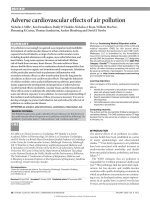
Fig. 4. Correlation between TSPM and PM
10
Concentration.

y = 719.98e
-0.0035x
R
2
= 0.9957
0
100
200
300
400
500
600
700
800
0 100 200 300 400 500 600
Distance along Down Wind Direction, meters
Predicted Values of TSPM
Concentration, (µg/m3)
Predicted TSPM
Concentration
Expon. (Predicted
TSPM Concentration)

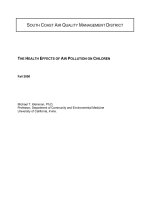
Fig. 5. Relation of TSPM Concetration with Distance from OCP.

0
200
400
600
800

1000
1200
Filter
Plant
Kitadi
Village
Manager
Office Sec
-IV
Sampling Sites
TSPM Concentration
(µg/m
3
)
Observed Values of TSPM (µg/m3) Predicted Values of TSPM (µg/m3)

Fig. 6. Comparision between Observedvalues and Predicted Values of TSPM.

Species Name Family Local Name of
Plants
Evergreen (E) or
deciduous
Butea monsperma Moraceae Palas Deciduous
Spathodea companulata Bignoniaceae Sapeta Evergreen
Fiscus infectoria Moraceae Pakur Evergreen
Cassia fistula Caesalpiniaceae Amaltas Deciduous
Anthocephalus cadamba Rubiaceae Kadam Deciduous
Cassia siamea Caesalpiniaceae Minjari Deciduous
Table 7. Recommended pollution retarding plant species for green belt development

Monitoring, Control and Effects of Air Pollution

12
4. Conclusions
TSPM and PM
10
are the major sources of emission from various opencast coal mining
activities. The predicted values of TSPM using FDM are 70 percent to 94 percent of observed
values. The difference between observed values and predicted values of TSPM indicates that
there are non-mining sources of emission viz. domestic transportation network near by mine
sites and other industries etc. Fugitive Dust Model (FDM) has been found to be most
suitable for modeling of dispersion pattern of fugitive dust at Padampur Opencast Coalmine
Project of W.C.L. PM
10
is the main focus of concern for human health. Correlation between
PM
10
and TSPM would help in predicting the PM
10
concentration by knowing the
concentration of TSPM for a similar mining site. Maximal concentration of TSPM is found in
a mining area and the concentrations falls exponentially with increase in distance due to
transportation, deposition and dispersion of particles.
Of the various sources of TSPM pollution, line sources contribute more than other sources
because of their lengths and nature of mining operations. Among the line sources, emission
rates have been in case of haul found and transport road to be 0.0127 gm per meter per
second and 0.0132 gm per meter per second respectively. Emission rate for whole mine is
found 0.0000108 gm per sq. meter per second. Various management strategies are evaluated
for reduction of dust emission at the source and design of green belt with few recommended
species is also very effective tool to mitigate air pollution. Proper dust suppression

arrangement is to be made including installation of continuous atomized spraying system
for haul roads and transport roads. As exposed overburden dump is another major
contributor of pollution load, judicious, plantation on these dumps is highly recommended.
However, for achieving the effective result to bring down the air pollution level in the
mining area a constructive measure at political level is also highly essential. This would lead
to an eco-friendly mining and better habitat for all those living in the area.
5. Acknowledgements
Authors are grateful to the Director, Central Institute of Mining and Fuel Research (CIMFR),
Dhanbad, India for giving permission to publish this article. Authors are also thankful to
M/s Western Coalfields Limited, Nagpur for sponsoring this study and providing necessary
facilities.
6. References
Almbauer, R.A., Piringer, M., Baumann, K., Oettle D., & Sturm P.J. (2001). Analysis of the
daily variations of winter time air pollution concentrations in the city of Graz,
Austria., Environmental Monitoring and Assessment, Vol. 65, pp. 79–87.
Appleton, T.J., Kingman, S.W., Lowndes I.S., & Silvester, S.A. (2006). The development of a
modeling strategy for the simulation of fugitive dust emissions from in-pit
quarrying activites: a UK case study, International Journal of Mining, Reclamation and
Environment, Vol. 20, P. 57-82.
Baldauf, R.W., Lane D.D., & Marote, G.A. (2001). Ambient air quality monitoring network
design for assessing human health impacts from exposures to air-borne
contaminants, Environmental Monitoring and Assessment, Vol. 66, pp. 63–76.
Banerjee, S.P (2006). TSP emission factors for different mining activities for air quality
impact prediction as collated from different sources, Minetech, Vol. 27, pp. 3-18.
CPCB, Central Pollution Control Board Notification, India, (1994).
Generation and Dispersion of Total Suspended Particulate
Matter Due to Mining Activities in an Indian Opencast Coal Project

13
Chaulya, S.K., Chakraborty, M.K., & Singh R.S.(2001). Air pollution modelling for a

proposed limestone quarry. Water, Air, and Soil Pollution Vol. 126, pp. 171–191.
Chaulya, S. K. (2004). Assessment and management of air quality for an opencast coal
mining area, Journal of Environmental Management, Vol. 70, No. 1, pp. 1-14
CIMFR. Central Institute of Mining and Fuel Research (erstwhile Central Mining Research
Institute) Report (1998). Determination of Emission Factor for Various Opencast
Mining Activities, GAP/9/EMG/MOEF/97, Dhanbad, India
Collins, M.J., Williams P.L, & MacIntosh, D.L (2001). Ambient air quality at the site of a
former manufactured gas plant. Environmental Monitoring and Assessment Vol. 68,
pp. 137–152.
Corti, A. & Senatore, A. (2000). Project of an air quality monitoring network for industrial
site in Italy. Environmental Monitoring and Assessment, Vol. 65, pp. 109–117
Crabbe, H., Beaumont R. & Norton, D. (2000). Assessment of air quality, emissions and
management in a local urban environment. Environmental Monitoring and
Assessment, Vol. 65 , pp. 435–442.
Cole, C.F. & Zapert, J.C. (1995).Air Quality Dispersion Model Validation at Three Stone
Quarries, Washington DC, National Stone Association.
Ghose, M.K. & Majee, J. (2000). Assessment of dust generation due to opencast coal
mining—an Indian case study. Environmental Monitoring and Assessment, Vol. 61,
pp. 255–263.
Ghose, M.K. & Majee, S.R. (2000). Assessment of the impact on the air environment due to
opencast coal mining -an Indian case study, Atmospheric Environment ,Vol. 34, pp.
2791-2796
Gilford, F.A. (1961). Uses of Routine Meteorological Observations for estimating
atmospheric Dispersion, Nuclear Safe, Vol. 2
Grundnig, P.W., Höflinger, W., Mauschitz, G., Liu, Z., Zhang G., & Wang, Z. (2006).
Influence of air humidity on the suppression of fugitive dust by using a water-
spraying system, China Particuology, Vol. 4, No. 5, pp. 229-233.
Hanna, S.R., Briggs, G.A. &. Hosker, R.P. (1982). Handbook on Atmospheric Diffusion,
DOE/TIC-11223, US Department of Energy, Technical Information Center
Jones, T. Blackmore, P. Leach, M. Matt, B.K. Sexton K. &. Richards, R. (2002). Characterisation

of airborne particles collected within and proximal to an opencast coalmine: South
Wales. UK Environmental Monitoring and Assessment, Vol. 75, pp. 293–312.
Kapoor, R.K. &. Gupta, V.K., (1984). A pollution attenuation coefficient concept for
optimization of green belt. Atmospheric Environment, Vol. 18, pp. 1107–1117.
Karaca, M., Tayanc M. &. Toros, H. (1995). The effects of urbanization on climate of Istanbul
and Ankara: a first study. Atmospheric Environment, Vol. , pp. 3411–3429.
Kumar, C.S.S., Kumar, P., Deshpande, V.P., &. Badrinath S.D. (1994). Fugitive dust emission
estimation and validation of air quality model in bauxite mines, Proceedings of
International Conference on Environmental Issues in Minerals and Energy Industry, IME
Publications, New Delhi, India, pp. 77–81.
Muleski G.E. &. Cowherd, C. (1987). Evaluation of the effectiveness of Chemical dust
Suppressants on Unpaved Roads, EPA/600/2-87.102. U.S. Environmental Protection
Agency, Research Triangle Park N.C., pp-81.
Pandey, S.K., Tripathi, B.D. &. Mishra, V.K. (2008). Dust deposition in a sub-tropical
opencast coalmine area, India, Journal of Environmental Management, Vol. 86, No. 1,
pp. 132-138.
Pasquill, F. (1962). Atmospheric Diffusion, Van Nostrand Co. Ltd. Londan

Monitoring, Control and Effects of Air Pollution

14
Peavy, H.S., Rowe, D.R. &. Obanoglous, G. Tech (1985). Environmental Engineering, Megraw
Hill, New York, pp. 668-670.
Reddy, G.S. &. Ruj, B. (2003). Ambient air quality status in Raniganj–Asansol area, India.
Environmental Monitoring and Assessment, Vol. 189, pp. 153–163.
Roney J. A. &. White, B. R. (2006). Estimating fugitive dust emission rates using an
environmental boundary layer wind tunnel, Atmospheric Environment, Vol. 40, pp.
7668-7685
Shannigrahi, A.S. &. Sharma, R.C. (2000). Environmental factors in green belt development-
an overview. Indian Journal of Environmental Protection , Vol. 20, pp. 602–607.

Sharma, S.C. &. Roy, R.K. (1997). Green belt—an effective means of mitigating industrial
pollution. Indian Journal of Environmental Protection Vol. 17, pp. 724–727.
Sinha, S. &. Banerjee, S.P. (1997). Characterisation of haul road in Indian open cast iron ore
mine. Atmospheric Environment, Vol. 31, pp. 2809–2814.
Tayanc, M. (2000) An assessment of spatial and temporal variation of sulphur dioxide levels
over Istanbul, Turkey. Environmental Pollution, Vol. 107, pp. 61–69.
Tichy, J. (1996). Impact of atmospheric deposition on the status of planted Norway space
stands: a comparative study between sites in Southern Sweden and the North
Eastern Czech Republic. Environmental Pollution, Vol. 93, pp. 303–312
Triantafyllou, A.G. (2003). Levels and trends of suspended partcles around large lignite
power station. Environmental Monitoring and Assessment, Vol. 89, pp. 15–34.
Triantafyllou, A.G., Kyros E.S. &. Evagelopoulos, V.G. (2002). Respirable particulate matter
at an urban and nearby industrial location: concentrations and variability, synoptic
weather conditions during high pollution episodes. Journal of Air and Waste
Management Association, Vol. 52, pp. 287–296.
Trivedi, R. Chakraborty M. K., &. Tiwary, B.K. (2009). Dust Dispersion Modeling Using
Fugitive Dust Model at an Opencast Coal Project of Western Coalfields Limited,
India, Journal of Scientific and Industrial Research, Vol. 68, pp71-78
Turner, D.B. (1970).Workbook of atmospheric Dispersion Estimates, U.S.E.P.A.,Washington, DC.
USEPA, United States Environmental Protection Agency (1995). User's guide for the fugitive
dust model (FDM), vol. 1, User Instructions, Region 10, 1200 sixth Avenue, Seattle,
Washington, USA.
Vallack, H.W. &. Shillito, D.E. (1998). Suggested guidelines for deposited ambient dust,
Atmospheric Environment, Vol. 32, No. 16, pp. 2737–2744.
Wheeler, A.J., Williams, I. Beaumont, R.A., &. Manilton, R.S. (2000). Characterisation of
particulate matter sampled during a study of children's personal exposure to air
borne particulate matter in a UK urban environment. Environmental Monitoring and
Assessment, Vol. 65, pp. 69–77.

2
Secondary Acidification
Mizuo Kajino
1
and Hiromasa Ueda
2

1
Meteorological Research Institute, Japan Meteorological Agency,
2
Toyohashi Institute of Technology,
Japan
1. Introduction
Secondary acidification (Kajino et al., 2008), also referred to as indirect acidification (Kajino et
al., 2005; Kajino & Ueda, 2007), is a process that involves accelerated acid deposition associated
with changes in gas–aerosol partitioning of semivolatile aerosol components, such as nitric
acid (HNO
3
), hydrochloric acid (HCl), and ammonia (NH
3
), even though emissions of these
substances and their precursors (e.g., NO
x
) remain unchanged. HNO
3
, HCl, and NH
3
are
thermodynamically partitioned into gas and aerosol (particulate) phases in the atmosphere.
This partitioning depends on temperature, humidity, and the presence of other components

such as sulfuric acid (H
2
SO
4
) and crustal cations (Na
+
, Mg
2+
, Ca
2+
, and K
+
). Among acidic
components in the air, H
2
SO
4
has an equilibrium vapor pressure very much lower than that of
other acids. When H
2
SO
4
concentrations increase, NO
3
-
and Cl
-
in the aerosol phase shift to the
gas phase, which causes the concentrations (fractions) of gaseous HNO
3

and HCl to increase,
although total nitrate (t-NO
3
= HNO
3
+ NO
3
-
) and total chloride (t-Cl = HCl + Cl
-
) remain
unchanged. The deposition velocities of the highly reactive gaseous phases of HNO
3
and HCl
are larger than those of their aerosol phases. For example, measured dry deposition velocities
of HNO
3
gas are 20 times those of NO
3
-
aerosols (Brook et al., 1997). Moreover, HNO
3
and HCl
gases both readily dissolve into cloud and rain droplets. For solution equilibrium, their
Henry’s law constants are 2.1 × 10
5
and 727 mol L
-1
atm
-1

, respectively, which are extremely
large values compared with those of SO
2
and NO
2
(1.23 and 0.01 mol L
-1
atm
-1
, respectively).
Thus, below-cloud scavenging coefficients of irreversibly scavenged gases such as HNO
3
and
HCl are several times those of their corresponding aerosols (Jylhä, 1999a, 1999b). In-cloud
scavenging processes of gases and aerosols are hard to compare by this simple estimation
procedure, because in-cloud scavenging of aerosol phases involves complexity of cloud
dynamical and microphysical processes. Model calculations supported by observational data
are necessary to estimate which phases are more efficiently scavenged for determination of net
(in-cloud and below-cloud) wet deposition.
The secondary acidification effect was first identified in volcanic SO
2
plumes
(Satsumabayashi et al., 2004). Miyakejima volcano, 180 km south of Tokyo, has erupted
continuously since July 2000, resulting in considerable SO
2
emissions into the troposphere.
One year after the start of emissions measurement in September 2000 (Kazahaya, 2001), SO
2

emissions totaled 9 Tg, equivalent to half the 20 Tg of anthropogenic SO

2
emissions from
China in 2000. According to ground-based observations of gases and aerosols at Happo
Ridge observatory (1,850 m ASL, 300 km north of Miyakejima volcano), the fraction of
gaseous HNO
3
and HCl in the Miyakejima volcanic plume exceeded 95% (September 2000),

Monitoring, Control and Effects of Air Pollution

16
whereas in the same season the fraction of these gases in contaminated air masses of the
Asian continental outflow was approximately 40% (September, 1999). Consequently, the
bimonthly mean NO
3
-
and Cl
-
concentrations in precipitation (net wet deposition) in August
and September 2000 at Happo Ridge, after the eruption, increased by 2.7 and 1.9 times,
respectively, compared with the same months in 1999, before the eruption.
Extensive studies of the seasonal and diurnal variations in gas–aerosol partitioning of
semivolatile components and the mechanisms causing partitioning changes have been
conducted (Moya et al., 2001; Lee et al., 2006; Morino et al., 2006). It was confirmed that the
partitioning importantly influences surface fluxes of pollutants (Nemitz and Sutton, 2004)
and climate (Adams et al., 2001; Schaap et al., 2004). The current study series on secondary
acidification provides new evidence that changes in the gas–aerosol partitioning have
important environmental impacts.
In section 2, we describe the secondary acidification process in detail. We present the results of
our previous study series on secondary acidification due to the Miyakejima volcanic eruption

in section 3, based on observational evidence (sect. 3.1) and modeling (sect. 3.2). In section 4,
we describe secondary acidification occurring during long-range transport of anthropogenic
air pollutants. We conduct an observational analysis (sect. 4.1) to reveal the current status, and
perform model studies (sect. 4.2) to analyze possible future scenarios. We summarize our
major findings in section 5. Here, we focus mainly on accelerated deposition of nitrate rather
than that of chloride, because anthropogenic chloride emissions contain large uncertainty.
2. Secondary acidification process
Secondary acidification is defined as the process by which acid deposition is indirectly
accelerated in association with changes in the gas–aerosol partitioning of semi-volatile
atmospheric constituents, such as nitric acid, hydrochloric acid, and ammonia, even though
emissions of these species and their precursors remain constant.


Fig. 1. Schematic illustration of secondary acidification by nitric acid. Values shown in the
figure are those observed during the Miyakejima volcanic eruption event, discussed in
section 3.1.

Secondary Acidification

17
Gas–aerosol equilibrium of semi-volatile inorganic components in solid
aerosols
Reaction
No.
NH
3
(g) + HNO
3
(g) ↔ NH
4

NO
3
(s) (R1)
NH
3
(g) + HCl(g) ↔ NH
4
Cl(s) (R2)
Gas–aerosol equilibrium of semi-volatile inorganic components in liquid
aerosols

NH
3
(g) + HNO
3
(g) ↔ NH
4
+
+ NO
3
-
(R3)
NH
3
(g) + HCl(g) ↔ NH
4
+
+ Cl
-
(R4)

As sulfuric acid gas increases via photochemical oxidation of SO
2

SO
2
(g) + OH radical (g) → H
2
SO
4
(g) (R5)
H
2
SO
4
(g) + NH
3
(g) → NH
4
HSO
4
(p) (R6)
H
2
SO
4
(g) + 2NH
3
(g) → (NH
4
)

2
SO
4
(p) (R7)
As sulfate increases via aqueous-phase oxidation
1
S(IV) + O
3
(aq) → S(VI) + O
2
(R8)
HSO
3
-
+ H
2
O
2
(aq) → SO
4
2-
+ H
2
O (R9)
SO
4
2-
+2NH
4
+

↔ (NH
4
)
2
SO
4
(R10)
In the presence of sea-salt particles
2NaCl + H
2
SO
4
(g) → Na2SO
4
+ HCl(g) (R11)
NaCl + HNO
3
(g) → NaNO
3
+ HCl(g) (R12)
In the presence of calcite-rich dust particles
CaCO
3
+ H
2
SO
4
(g) → CaSO
4
+ H

2
O + CO
2
(g) (R13)
CaCO
3
+ HNO
3
(g) → Ca(NO
3
)
2
+ H
2
O + CO
2
(g) (R14)
1. S(IV) ≡ SO
2 ⋅
H
2
O, HSO
3
-
, and SO
3
2-
; S(VI) ≡ HSO
4
-

and SO
4
2-

Table 1. Chemical reactions describing the changes in gas–aerosol partitioning of semi-
volatile inorganic components involved in the secondary acidification process.
Figure 1 illustrates schematically secondary acidification effects of nitric acid caused by
increases in SO
2
emissions. The values used in Figure 1 are those measured at the Happo
Ridge observatory and on Miyakejima Island, and reflect secondary acidification effects due
to the eruption of Miyakejima volcano (see section 3.1 for details). Table 1 summarizes
typical chemical reactions between atmospheric constituents involved in the secondary
acidification process. Nitric acid is partitioned into HNO
3
gas and NO
3
-
aerosol in the
atmosphere (Figure 1, panel 1; R1 and R3 in Table 1). Since the partitioning is sensitive to
temperature, over East Asia the gas phase is dominant in summer and at lower altitude,
whereas the aerosol phase is dominant in winter and at higher altitude (Morino et al., 2006;
Hayami et al., 2008; Kajino et al., 2008). This partitioning is also altered by the presence of
other inorganic components. Hereafter, for simplicity, we focus on thermodynamic
equilibrium in the NH
3
–HNO
3
–H
2

SO
4
–H
2
O system. An increase in SO
2
emissions (Figure 1,
panel 2), is followed by the oxidation of SO
2
[S(IV)] to S(VI), that is, either to H
2
SO
4
gas by a
gas-phase photochemical reaction (R5), or to SO
4
2-
by aqueous-phase reactions (R8 and R9)
in liquid aerosol or rain droplets. Because the vapor pressure of H
2
SO
4
gas is extremely low,
ammonium sulfate aerosols form immediately (R6 and R7). In the aqueous phase, SO
4
2-
,
because it is a strong acid, forms an ion pair with NH
4
+

(R10). Because sulfate consumes
ammonia in the gas phase, the equilibrium of (R1 and R3) shifts leftward, and, as a result,
HNO
3
gas evaporates from the aerosol phase (Figure 1, panel 3).
Wet and dry deposition rates of the highly reactive gaseous HNO
3
are high (Seinfeld and
Pandis, 2006). Thus, as the SO
4
2-
concentration increases, the concentration fraction of HNO
3


Monitoring, Control and Effects of Air Pollution

18
increases, with the result that deposition of total nitrate (t-NO
3
= HNO
3
+ NO
3
-
) is enhanced,
even though the total nitrate concentration, as well as that of its precursors (i.e., NO
x
),
remains unchanged.

In the presence of abundant sea salt or mineral dust particles, however, HNO
3
gas is
deposited on particle surfaces, expelling Cl
-
and CO
3
-
, respectively, into the gas phase (R12
and R14). Na
+
from sea salt and Ca
2+
from mineral dust particles can also be counterions of
SO
4
2-
(R11 and R13). In such cases, increases in the gas phase fraction of t-NO
3
due to
increased SO
4
2-
and subsequent consumption of NH
3
are suppressed (see also section 4.1
and Kajino et al., 2008).
3. Eruption of Miyakejima volcano and the resulting secondary acidification
effects in Japan
The eruption of Miyakejima volcano (Mt. Oyama, 139°32′E, 34°05′N, summit elevation 815 m

ASL; Figure 2), 180 km south of Tokyo, Japan, beginning in July 2000 has resulted in the
emission of huge amounts of sulfur dioxide. The annual mass of sulfur dioxide emitted was
vast (9 Tg yr
-1
; Kajino et al., 2004), equivalent to half the annual anthropogenic emission from
China in 2000 (20 Tg yr
-1
, Streets et al., 2003). Gases, aerosols, and precipitation have been
sampled at the Happo Ridge observatory (137°48′E, 36°41′N, 1,850 m ASL, 330 km north of the
volcano; Figure 2) in the central mountainous region of Japan since May 1998, two years before
the eruption began (Satsumabayashi et al., 2004). Kajino et al. (2004, 2005) used a chemical
transport model to simulate the emission, transport, transformation, and deposition of
inorganic compounds such as SO
4
2-
, NO
3
-
, and NH
4
+
of anthropogenic and volcanic origin for
the one-year period from September 2000 to August 2001. In this section, we highlight the
outcomes of our previous research, focusing on the effects of the volcanic eruption on
concentrations and deposition of inorganic compounds over the far East Asian region.


Fig. 2. Map of Japan showing the locations of the Happo Ridge observatory, Miyakejima
volcano, the Tokyo Metropolitan Area, and the EANET monitoring stations Oki and Rishiri
(see section 4).

Secondary Acidification

19
3.1 Observational evidence
Temporal variations in smoke height (m) and SO
2
emissions (ton day
-1
) from Miyakejima
volcano (Figure 3) were measured with a correlation spectrometer (COSPEC) by the Japan
Meteorological Agency (Kazahaya, 2001). From the start of the observation, total measured
SO
2
emissions were 9 Tg yr
-1
, corresponding to about 70% of the global emissions from
volcanoes from the 1970s to 1997 (13 Tg yr
-1
; Andreas and Kasgnoc, 1998) and to about half
the anthropogenic SO
2
emitted from China in 2000 (20 Tg yr
-1
). The maximum emission,
about 82,200 ton day
-1
, was observed at 10:48 LT on 16 November 2000. This value is
equivalent to the anthropogenic emission from all of Asia in 2000 (34.3 Tg yr
-1

, ~94,000 ton
day
-1
; Streets et al., 2003). The observed smoke height on the same day was only 1,000 m,
indicating that almost the entire amount was released into the Planetary Boundary Layer.
The emission gradually decreased to about 10,000 ton day
-1
about 1 year after the onset of
eruption. In 2002, the emission was still substantial, at 16.8% of Chinese anthropogenic
emissions and 3.8 times Japanese anthropogenic emissions (Kajino et al., 2011). The
continuous injection of the volcanic plume containing SO
2
into the Planetary Boundary
Layer (i.e., the observed smoke height continued below 2,000 m) necessarily affected surface
air quality and environmental acidification over far East Asia substantially.
At Happo Ridge, aerosol samples are collected daily for 3 hours, from 12:00 to 15:00 LT,
with a high-volume air sampler. The four-stage filter pack method was used for intensive
sampling of gaseous and aerosol inorganic compounds during two weeks in September 1999
and one week in September 2000. Meteorological parameters and hourly concentrations of
SO
2
, NO
x
, O
3
, and PM
10
are monitored automatically. Satsumabayashi et al. (2004) have
described the observation methods in detail.

Fig. 3. Time series of observed smoke height (top) and SO
2
emissions (bottom) from
Miyakejima volcano. The data were interpolated using a spline function (solid lines) for use
as input in the model simulation.

Monitoring, Control and Effects of Air Pollution

20
Particle phase fraction
Sampling date and time
(LT)
SO
4
2-

mg m
-3

Nitrate Ammonium
Air mass of Asian continental origin before the eruption (1999)
13 Sep 12:00–15:00 12.3 0.60 0.78
13 Sep 15:00–18:00 12.1 0.61 0.77
13 Sep 18:00–21:00 8.80 0.57 0.76
13 Sep 21:00–24:00 8.10 0.82 0.72
14 Sep 00:00–03:00 10.7 0.50 0.74
Average 10.4 0.62 0.75
Air mass directly affected by the volcanic eruption (2000)
15 Sep 12:00–18:00 32.0 0.00 0.96

15 Sep 18:00–24:00 20.3 0.00 0.94
16 Sep 00:00–06:00 11.0 0.17 0.76
16 Sep 06:00–12:00 6.40 0.00 0.75
Average 17.4 0.04 0.85
Table 2. Gas–aerosol partitioning observed at Happo Ridge before and after the onset of the
eruption.
We selected two high sulfate concentration events, from 12:00 LT 13 September to 3:00 LT 14
September 1999, before the onset of the eruption, and from 12:00 LT 15 September to 12:00
LT 16 September 2000, just after the onset of the eruption, and examined SO
4
2-

concentrations and gas–aerosol partitioning of t-NO
3
and t-NH
4
(= NH
3
+ NH
4
+
) measured
at Happo Ridge (Table 2). Prior to the eruption, in September 1999, the gas–aerosol
partitioning of nitrate in the contaminated air mass from the Asian continent tended to favor
the aerosol phase: 62% in the aerosol phase versus 38% in the gas phase (Figure 1, panel 1).
Similarly, the gas–aerosol partitioning of ammonia also favored the aerosol phase (72%
aerosol, 25% gas). In September 2000, two months after the onset of eruption, the gas–
aerosol partitioning of nitrate in the air mass from Miyakejima Island was biased almost
entirely toward the gas phase (4% aerosol, 96% gas), whereas the aerosol phase fraction of
ammonium was higher (85%) than it was before the eruption onset. This result is consistent

with thermodynamic equilibrium theory (Table 1).
Table 3 lists the mean bimonthly concentrations of trace chemical components in gases,
aerosols, and precipitation measured at Happo Ridge before and after the onset of the
eruption. After the eruption, the concentrations of SO
2
gas, SO
4
2-
aerosol, and SO
4
2-
in
precipitation increased dramatically, by 15, 3, and 6.8 times, respectively, compared with their
concentration before the eruption. The concentration of NH
4
+
, a major counterion of SO
4
2-
in
aerosols doubled, and it increased in precipitation, by 5 times after the eruption. O
3
and PM
10

(aerosols smaller than 10μm in diameter) concentrations were slightly higher in September
2000 than before the eruption, but the difference was small compared with the concentration
differences in inorganic compounds, indicating that photochemical activity and the total
aerosol concentrations were not very different between the period before and that after the
eruption began. However, NO

3
-
in precipitation increased by 2.7 times after the eruption,
whereas aerosol NO
3
-
concentrations did not differ between the two periods. Unfortunately,
continuous measurement data for HNO
3
gas are not available, so t-NO
3
cannot be determined.
Because secondary acidification is defined as an increase in NO
3
-
deposition while the t-NO
3

concentration remains unchanged, we cannot prove that the observed increase in bimonthly

Secondary Acidification

21
mean NO
3
-
in rainwater was caused by secondary acidification. Nevertheless, the observations
are consistent with secondary acidification theory.

Gas, ppb

Aerosol, μg m
-3

Precipitation, mg L
-1


SO
2
O
3
PM
10
SO
4
2-
NO
3
-
NH
4
+
SO
4
2-
NO
3
-
NH
4

+

Before eruption
(Aug. and Sep. 1999)
0.2 38 14 2.2 0.2 0.75 0.25 0.31 0.06
After eruption
(Aug. and Sep. 2000)
3.3 46 17 6.5 0.24 1.56 1.70 0.83 0.33
Table 3. Mean bimonthly concentrations of various components of gases, aerosols, and
precipitation measured at Happo Ridge before the onset of the eruption and one year later.
It has still not been proved whether wet scavenging of HNO
3
gas or of NO
3
-
aerosol is more
efficient. Because Henry’s law constant of HNO
3
is extremely large and below-cloud
scavenging of aerosols is not very efficient, the below-cloud scavenging coefficient of HNO
3

is several times the size of the aerosol scavenging coefficients (Jylhä, 1999a, 1999b). In-cloud
aerosol scavenging is much more efficient because the aerosol particles act as cloud
condensation nuclei (CCN). HNO
3
can also dissolve in cloud droplets, however, so it is
likely that wet scavenging of HNO
3
is more efficient than that of NO

3
aerosols.
Because no methods are available for quantitative measurement of wet scavenging
efficiency, numerical models that incorporate cloud dynamical and microphysical processes
must be used to determine the wet scavenging efficiency of HNO
3
compared with that of
NO
3
aerosols. However, because such models require many assumptions and several
parameterizations, especially for modeled gas–aerosol–cloud interaction processes, the
numerical answer includes substantial uncertainty. Thus, the results require careful
interpretation. In the next section, the simulation results for secondary acidification effects
due to the eruption of Miyakejima Volcano are discussed.
3.2 Model simulations
Kajino et al. (2005) investigated secondary acidification due to the Miyakejima eruption over
the one-year period from September 2000 to August 2001 by using a chemical transport
model (MSSP, Model System for Soluble Particles; Kajino et al., 2004). They concluded that
dry and wet deposition of nitrate increased by 0.2–0.8 and 0.5–4 mg m
-2
day
-1
, respectively,
over far East Asia on average during the year. However, the MSSP model does not include
an aerosol dynamics module, and it assumes thermodynamic equilibrium of semi-volatile
inorganic compounds. Therefore, we recently developed a more sophisticated aerosol
chemical transport and deposition model, and then used the new model to revisit the
volcanic eruption study and examine secondary acidification effects of the plume.
The new aerosol chemical transport model used for the simulation is called Regional Air
Quality Model 2. In RAQM2, a simple version of a modal-moment aerosol dynamics model

(MADMS; Kajino, 2011) was implemented to achieve a completely dynamical (non-
equilibrium) solution for gas-to-particle mass transfer over a wide range of aerosol
diameters, from 1 nm to greater than 1 μm. MADMS is unique in that it is capable of solving
inter-modal coagulation between two modes with very different log-normal size
parameters. To consider a variety of atmospheric aerosol properties, including size,
chemical composition, and mixing states, a category approach of the EMTACS (Eulerian

Monitoring, Control and Effects of Air Pollution

22
Multiscale Tropospheric Aerosol Chemistry and dynamics Simulator) model (Kajino and
Kondo, 2011) is utilized. The Advanced Research WRF (Weather Research and Forecasting)
model (version 3.1.1; Skamarock et al., 2008) is used to simulate the meteorological field.
Lateral and upper boundary concentrations used for the RAQM2 simulation were hourly
concentrations of NO
x
, O
x
, CO, and volatile organic carbons simulated by a global-scale
stratospheric and tropospheric chemical climate model (MRI-CCM2; Deushi and Shibata,
2011). Thus, RAQM2 is a so-called one-way nested model of the global chemistry model.
The RAQM2 used Streets et al. (2003)’s anthropogenic emission inventory as well as other
sources of aerosol emissions such as biogenic sources, open biomass burning, and wind-
generated emissions (dust and sea-salt). The model domain is illustrated in Figure 4. There
are 100 × 70 horizontal grids, and the resolution is 60 km with a Lambert conformal conic
map projection and a reference latitude/longitude of 35°N/115°E. Vertically, there are 28
layers from the ground to 100 hPa in WRF, and 13 layers from the ground to 10 km in
RAQM2, with terrain-following coordinates.

Fig. 4. The WRF and RAQM2 model domain, topography used in the model (color scale, m
ASL), and locations of important geographical features.
The simulations were conducted for the month of October 2000. Since wind and
precipitation patterns change seasonally, the concentrations and deposition patterns of air
pollutants vary substantially during a year. We selected October 2000 for the simulation
because during that month volcanic emission was active and the volcanic plume was carried
to the Japan archipelago. The Miyakejima volcanic emissions are injected into horizontal
grid (X = 87, Y = 39), which corresponds to the location of Miyakejima volcano (Mt. Oyama,
139°32′E, 34°05′N). The SO
2
emission flux and injection height were estimated by spline
interpolation of the measured data (solid lines in Figure 3; ~30,000 ton day
-1
) and uniformly
distributed to the vertical grids (Z ≈ 5–7) corresponding to the interval from the summit
elevation (815 m ASL) to the measured smoke height (~1,500 m above the crater).
Figure 5 illustrates monthly mean surface concentrations of anthropogenic and volcanic SO
2

and SO
4
2-
(volcanic data were derived by subtracting the simulation result obtained without
including volcanic emissions from that obtained with volcanic emissions), the gas-phase
fraction of t-NO
3
, and its increase due to increased volcanic SO
4
2-
in October 2000. The

volcanic SO
2
concentration over the area downwind of the volcano (Figure 5b) was




Secondary Acidification

23

Fig. 5. Spatial distributions of anthropogenic (a and c) and Miyakejima volcanic (b and d)
monthly mean surface concentrations of (a and b) SO
2
(ppb) and (c and d) SO
4
2-
(μg m
-3
). (e)
The gas-phase fraction of t-NO
3
(%) and (f) its increase due to the volcanic eruption (%) in
October 2000.
comparable to the anthropogenic SO
2
concentration over the continent, whereas the
anthropogenic concentration over Japan was much less (Figure 5a). Because SO
4
2-

is
produced by oxidation of SO
2
during transport, SO
4
2-
is widely distributed over the
downwind areas (Figures 5c and 5d). The maximum concentration of volcanic SO
4
2-
was
smaller than that over the land, probably because photochemical oxidants such as OH
radicals, O
3
, and H
2
O
2
are more abundant over the continent. In central Japan, the SO
4
2-

concentration was doubled as a result of the volcanic eruption. The gas phase fraction of t-
NO
3
was smaller over the continent (1–15%) than over the ocean or the Japan archipelago
(20–40%) (Figure 5e), because the surface temperature is higher over the ocean than over the
continent in October. These values are consistent with those observed at Happo Ridge.
Expulsion of NO
3

-
from the aerosol phase occurred as a result of the volcanic SO
2
emission,

Monitoring, Control and Effects of Air Pollution

24
with an increase of the gas-phase fraction of about 2–5% (Figure 5f). The gas-phase fraction
is small compared with the observed fraction at Happo Ridge, where the gas-phase fraction
reached 100% during volcanic plume transport events. It is probably because simulated
ammonia concentration is overestimated so that it fixed HNO
3
in the aerosol phase and
inhibited the expulsion of NO
3
-
due to increased sulfate.
Figures 6a-d illustrates the monthly cumulative dry and wet deposition of t-NO
3
in October
2000 and changes due to the volcanic eruption. Figures 6e and 6f show monthly
precipitation over East Asia and around Japan, respectively. Secondary acidification in dry
deposition, that is, the increase of nitrate in dry deposition, in the region downwind of the
Miyakejima volcano, is evident (0.5–3 mg m
-2
) accounting for at maximum about 10% of the
total amount (20–80 mg m
-2
).

Fig. 6. Spatial distributions of cumulative monthly dry deposition of (a) total nitrate (gas +
aerosol) (mg m
-2
) and (b) the difference due to the eruption. (c and d) The same as (a) and (b)
but for wet deposition (mg m
-2
). (e and f) Monthly cumulative precipitation (mm) in October
2000.

Secondary Acidification

25
Secondary acidification due to wet deposition was rather complex. An increase in nitrate in
wet deposition was simulated over the central Japan land mass (5–10 mg m
-2
), whereas a
decrease of 2–15 (mg m
-2
) was simulated over the ocean south of the archipelago, where
precipitation was heavier. The decrease is due probably to dominance of in-cloud
scavenging of aerosols (NO
3
-
acting as CCN) over the dissolution of HNO
3
gas, so that the
increased fraction of HNO
3

resulted in a decrease in the wet deposition of t-NO
3
.The
modeled wet deposition increase was smaller than that predicted by MSSP (15–120 mg m
-2
),
which simulated that an increase in the wet deposition of nitrate was comparable to that of
sulfate (see Area 1, October 2000 in Table 3 of Kajino et al., 2005).
Even though the RAQM2 model is more sophisticated than the MSSP model, it is hard to
judge which model results are closer to reality. MSSP does not solve aerosol processes
dynamically. The aerosol size distribution is diagnosed as a simple function of relative
humidity, and all particles of inorganic compounds such as SO
4
2-
, NO
3
-
, and NH
4
+
are
assumed to act as CCN and to become dissolved in cloud droplets (Kajino et al., 2004). In
contrast, the more sophisticated RAQM2 model solves the evolution processes
(condensation, evaporation, and coagulation) of the aerosol size distribution dynamically for
aerosol diameter ranges from 1 nm to greater than 1 µm. Then, the CCN activity of particles
is calculated using the parameterization of Abdul-Razzak and Ghan (2000). This
parameterization was developed from cloud parcel model calculations, including aerosol–
cloud interaction processes. The critical diameter D
c
(above which aerosol particles can act

as CCN) is calculated from the predicted aerosol size distribution and chemical composition,
the temperature and humidity in the environment, and the updraft velocity. Ironically,
however, because it is quite challenging to reproduce atmospheric aerosol size distributions,
especially for sub-micron particles, RAQM2 can fail to reproduce the CCN activity of
aerosols, which is very sensitive to particle size. Nevertheless, the simulated results of the
two models should not be far from reality, as the model results for various concentrations of
inorganic components in the air and in precipitation have been evaluated extensively using
measurement data (Kajino et al., 2011, and references therein; Kajino and Kondo, 2011).
4. Secondary acidification as a result of long-range transport over East Asia
In section 3, we showed that secondary acidification occurred during an extreme episode. In
this section, we investigate secondary acidification under general air pollution conditions.
Asia is one of the largest anthropogenic SO
x
emitting regions in the world, and because of
the rapid economic growth in Asia, emissions there might change drastically in the future.
Therefore, understanding the impacts of secondary acidification in regions downwind of
large emission sources and how they change depending on future emission changes is
important. In section 4.1, we present indications of secondary acidification based on Acid
Deposition Monitoring Network in East Asia (EANET) data. In section 4.2, we use a
chemical transport model to simulate long-range transport of inorganic air pollutants over
the East Asian region. To evaluate the secondary acidification due to future emission
changes, we carried out simple sensitivity studies by increasing or decreasing emissions of
SO
2
and NH
3
, the gaseous counterparts of SO
4
2-
and NO

3
-
aerosols, in model simulations.
4.1 Observational evidence
We found indications of secondary acidification in the EANET monitoring data. EANET began
collecting data on a regular basis in 2001, following established guidelines and technical

Monitoring, Control and Effects of Air Pollution

26
procedures and adopting a quality assurance/quality control program (EANET, Guidelines
for Acid Deposition Monitoring in East Asia; available from
In 2002, two additional Japanese monitoring stations
began to measure concentrations of gas and aerosol components by the filter pack (FP)
method, increasing the number of monitoring stations in Japan to the current 10. At these
stations, 7- or 14-day cumulative concentrations of gaseous species (HNO
3
, HCl, NH
3
, SO
2
)
and aerosol components (SO
4
2-
, NO
3
-
, Cl
-

, NH
4
+
, Na
+
, Mg
2+
, K
+
, Ca
2+
) are monitored, and 1-day
cumulative concentrations in precipitation (SO
4
2-
, NO
3
-
, Cl
-
, NH
4
+
, Na
+
, Mg
2+
, K
+
, Ca

2+
) are
measured by collecting precipitation samples and analyzing them by ion chromatography.
The FP method is known to have several distinct artifact problems. Because particulate
NH
4
NO
3
and NH
4
Cl collected on a filter might volatilize during a 7- or 14-d sampling
period, there is a possibility that thermodynamic equilibrium may not have been attained. In
addition, high humidity can reduce the concentration of gaseous species because of trapping
by condensed water in the filter pack. To evaluate these sampling artifacts in the EANET FP
data, we employed a multicomponent gas–aerosol equilibrium model called Simulating
Compositions of Atmospheric Particles at Equilibrium (SCAPE; Kim et al., 1993; Meng et al.,
1995) to recalculate the gas–aerosol partitioning of t-NO
3
at six selected Japanese EANET
monitoring sites and compared the results with the measurement data (Kajino et al., 2008).
We found fairly high correlations, low mean errors, and low root mean square errors
between the observed and simulated values (see Table 2 of Kajino et al., 2008). We therefore
concluded that long-duration FP data from EANET are sufficiently consistent for detecting
the secondary acidification effect in our current analysis.
In the present study, we used monitoring data collected by two of the Japanese EANET
stations, Rishiri and Oki. As shown in Figure 2, these stations are situated on small islands
facing the Sea of Japan, so plumes from the continental outflow are efficiently detected.
Rishiri is further north than Oki, so the climate and air quality features differ between these
two stations.
Table 4 summarizes the monitoring results from Oki and Rishiri. Non-sea-salt (nss)-SO

4
2-
,
defined as the concentration difference between total [SO
4
2-
] and sea-salt-originated SO
4
2-

(= 0.251 × [Na
+
]) consists mostly of anthropogenic and partly of volcanic sulfate. Here, the
square brackets [ ] denote atmospheric concentration (μg m
-3
). C
nssS/N5
is the molar ratio of
nss-SO
4
2-
to the N(V) concentration, namely t-NO
3
, where C denotes the atmospheric
concentration. P
gHNO3
is the molar fraction of HNO
3
gas relative to t-NO
3

. F
s
, defined as,

2
2
2
4
[]
()
( ) ( ) [] []
SO
s
SO
nss SO
S
SIV
F
SIV nssSVI S S
−
−
≡=
++
(1)
is the ratio of tetravalent S to total (tetravalent plus hexavalent) anthropogenic S in the air.
Under the assumption that all SO
2
is of non-sea-salt origin, a low F
s
value indicates that SO

2
is
sufficiently oxidized to SO
4
2-
during long-range transport. D
N5/S6
/C
N5/S6
is the ratio of the N/S
molar ratio in precipitation to the atmospheric ratio (where D indicates wet deposition):

2
4
3
5/ 6 5/ 6
2
43 3
[]/96
[]
/
[][ ]/63[]/62
p
NS NS
gp
SO
dNO
DC
d SO HNO NO
−

−
−−
≡×
+
(2)
Here, d[ ] denotes the concentration in precipitation (μmol L
-1
), and the subscripts g and p
denote the gas phase and the particulate phase, respectively. As atmospheric concentrations

Secondary Acidification

27
were measured by the FP method on a 7- or 14-d cycle, the daily measured wet deposition
amounts are also averaged over the same sampling period.

Station name Oki Rishiri
Observation period 04/2003 – 03/2005 07/2002 – 03/2005
Number of samples 77 72
Longitude/Latitude 133.18/36.70 141.20/45.12

Mean concentration ± standard deviation, μg m
-3

[nss-SO
4
2-
] 3.54 ± 2.05 1.86 ± 0.95
[t-NO
3

] 1.21 ± 0.61 0.73 ± 0.47
[t-NH
4
] 1.26 ± 0.77 0.68 ± 0.34
[Crustals]
a
2.64 ± 1.58 2.31 ± 1.26
Mean meteorological measurements with standard
deviations
T, ºC 14.48 ±

7.17 6.50 ± 8.72
RH, % 74.10 ±

6.16 75.69 ± 6.00
Mean molar ratios with standard deviations
[nss-SO
4
2-
]/[SO
4
2-
] 0.86 ±

0.11 0.78 ±

0.13
C
nssS/N5
1.99 ±

1.06 1.96 ±

1.00
P
gHNO3
0.30 ±

0.22 0.20 ±

0.16
F
s
0.37 ±

0.16 0.34 ±

0.14
Correlation coefficient (R)
T versus P
gHNO3
0.63 0.46
C
nssS/N5
versus P
gHNO3
b
0.75 –0.03 → 0.41
P
gHNO3

versus D
N5/S6
/C
N5/S6
b
0.74 0.17 →

0.70
F
s
versus D
N5/S6
/C
N5/S6
b
–0.45 0.08 →

–0.43
a
[Crustals] = [Na
+
] + [Mg
2+
] + [K
+
] + [Ca
2+
]
b
The correlation coefficient R at Rishiri improved when it was calculated using only data collected when

[nss-SO
4
2-
]/[SO
4
2-
] > 0.8 and T > 0 °C .
Table 4. Information about Oki and Rishiri stations and monitoring results.

In general, Rishiri and Oki can be characterized as follows. Rishiri is located in northern
Japan where temperatures drop to below 0 °C in winter and the marine atmosphere is
relatively clean. Thus, the mean anthropogenic indicator [nss-SO
4
2-
]/[SO
4
2-
] was lower than
0.8. As the counterions of NO
3
-
, sea-salt-originated crustal concentrations of Na
+
and Mg
2+

were high (>2 μg m
-3
), resulting in a low P
gHNO3

(0.2) value. In contrast, Oki is located in
coastal western Japan, where it is influenced by Asian continental outflows, resulting in
relatively higher values of [nss-SO
4
2-
]/[SO
4
2-
] (>0.85) and P
gHNO3
(0.3). Relative humidity
(RH) did not differ significantly between the two stations.
Measured P
gHNO3
was positively correlated with T, as explained in section 2. We found a
slightly larger correlation between P
gHNO3
and C
nssS/N5
at Oki in western Japan, indicating a
marked expulsion of NO
3
-
by SO
4
2-
in the continental outflow. Conversely, at Rishiri the
correlation coefficient between P
gHNO3
and C

nssS/N5
was near zero, which we attributed to the
effects of abundant sea-salt components (R12). P
gHNO3
and D
N5/S6
/C
N5/S6
were positively
correlated at Oki. Here, D
N5/S6
/C
N5/S6
represents the N(V)/S(VI) molar concentration ratio

Monitoring, Control and Effects of Air Pollution

28
in precipitation to that in the atmosphere (Eq. 2). Accordingly, a positive correlation
between P
gHNO3
and D
N5/S6
/C
N5/S6
indicates a relatively higher wet deposition rate of t-NO
3
,
compared with that of S(VI), as the gas phase fraction of t-NO
3

increases, that is, secondary
acidification. Together with the positive correlation between C
nssS/N5
and P
gHNO3
, the
expulsion of particulate NO
3
-
to the gas phase by anthropogenic SO
4
2-
results in acceleration
of the wet deposition flux of t-NO
3
at Oki.
At Rishiri, where no correlation was detected between C
nssS/N5
and P
gHNO3
, analysis on the
basis of the D
N5/S6
/C
N5/S6
ratio is not applicable. Because of the abundance of cations of sea-
salt origin, the correlation coefficient between P
gHNO3
and D
N5/S6

/C
N5/S6
is 0.17. In addition,
the secondary acidification effect is usually based on the calculation of the vapor–liquid
equilibrium of semivolatile components, but Rishiri station is in northern Japan, where
precipitation during winter consists mostly of ice and snow rather than rain. Therefore, we
selected data sampled when the mean temperature exceeded 0 °C and [nss-SO
4
2-
]/[SO
4
2-
]
was greater than a threshold of 0.8, indicating less influence of sea-salt particles. The same
analysis using the selected samples resulted in an increase in the correlation coefficient
between C
nssS/N5
and P
gHNO3
from –0.03 to 0.41, and that between P
gHNO3
and D
N5/S6
/C
N5/S6

increased from 0.17 to 0.70. Secondary acidification is thus evident under the substantial
influence of anthropogenic contamination when the influence of sea-salt particles is low and
the temperature is sufficiently high for vapor–liquid equilibrium to be established.
Neutralization effects by the Asian dust particles (R14) may negate the increase in P

gHNO3

caused by the increase in SO
4
2-
. We thus performed a similar analysis using [nss-
Ca
2+
]/[Ca
2+
], but found no significant effects in the current data sets. Here, [nss-Ca
2+
] is
defined as the difference between total [Ca
2+
] and sea-salt-originated Ca
2+
(= 0.038 [Na+]);
therefore, higher values of [nss-Ca
2+
]/[Ca
2+
] would indicate the occurrence of Asian dust
events, which are characterized by abundant calcite.
Figure 7 shows the relationships between C
nssS/N5
and P
g-HNO3
(%), P
g-HNO3

(%) and
D
N5/S6/CN5/S6
, and F
s
and D
N5/S6/CN5/S6
at Oki and Rishiri. At Oki, the correlations are higher
because of its location in western Japan where it is influenced by the pronounced Asian
continental outflow. At Rishiri, however, the sea-salt effect is predominant, leading to very
weak correlations (open circles in Figs. 7d–f), although they are enhanced significantly by
sample selection for T > 0 °C and [nss-SO
4
2-
]/[SO
4
2-
] > 0.8 (closed circles).
It is notable that the regression lines obtained from the two stations are very similar despite
the ~1,200 km distance separating them. P
gHNO3
is less than 30% when C
nssS/N5
is less than 2
at Oki (Fig. 7a), whereas P
gHNO3
is often greater than 50% under the lower influence of sea-
salt particles (closed circles) when C
nssS/N5
is less than 2 at Rishiri (Fig. 7d). The slope of this

regression line for Rishiri is steeper than that for Oki, because the average concentration of t-
NH
4
, which can fix NO
3
-
as ammonium nitrate in the aerosol phase, is low at Rishiri, only
half the average concentration at Oki. However, when cations originating from sea salt are
abundant at Rishiri (open circles in Figure 7d), P
gHNO3
is less than 20%, even when C
nssS/N5
is
larger than 4.
The F
s
value is an indicator of the distance that pollutants have been transported. Relatively
short-distance transport within Japan is indicated by an F
s
value greater than approximately
0.6. Conversely, F
s
smaller than 0.2 indicates long-range transport from the Asian continent
to Japan (Satsumabayashi et al., 2004). At Oki, D
N5/S6/CN5/S6
was greater than 3 when F
s
was
smaller than 0.2 (Fig. 7c), indicating that secondary acidification effects were greater at Oki
when air pollutants had been transported a long distance. The same trend was observed for

the selected samples at Rishiri (closed circles, Fig. 7f).

Secondary Acidification

29

Fig. 7. Scattergrams of (a) C
nssS/N5
and P
gHNO3
, (b) P
gHNO3
and D
N5/S6
/C
N5/S6
, (c) F
s
and
D
N5/S6
/C
N5/S6
at Oki. (d–f) Same as (a–c) for Rishiri. The open circles in (a–f) show all data.
The closed circles in (d–f) show data of samples collected when T > 0 ºC and [nss-SO
4
2-
]/[SO
4
2-

] > 0.8. The solid regression lines in (d–f) are for all data, and the dashed regressions
lines are for only the data shown by the closed circles.

Monitoring, Control and Effects of Air Pollution

30
4.2 Model simulations
4.2.1 Future emission scenarios
In all four scenarios (A1, A2, B1, and B2) considered in the Special Report on Emissions
Scenarios (SRES) from the Intergovernmental Panel on Climate Change (IPCC) (2000),
emission rates are increasing faster in Asia than elsewhere in the world. In these scenarios,
SO
x
emissions in Asia are expected to peak between 2020 and 2050, becoming twice as high
as in 2000. NO
x
emissions will continue to increase even when SO
x
is no longer increasing,
reaching a maximum after 2040 at levels more than twice current levels in the lowest
estimation scenario (B1), and in the A2 scenario reaching a level approximately four times
the current level in 2100. SRES does not evaluate NH
x
emission rates, which have a marked
effect on gas–aerosol partitioning, but Klimont et al. (2001) estimated that NH
x
emissions
will increase to 1.7 times the 1995 level in East Asia by 2030.
Fujino et al. (2002) developed the AIM/Trend model (Asian-Pacific Integrated Model) to
assess future environmental loads based on past socio-economic trends. They estimated a

change in Asian SO
2
emissions from 30.8 Tg yr
-1
in 1998 to 21.9–85.1 Tg yr
-1
in 2032, depending
on the socio-economic scenario, Security First (SF), Market First, Sustainability First, or Policy
First. The largest emission growth ratio is estimated for the SF scenario, which assumes a
world of great disparities where inequality and conflict brought about by socio-economic and
environmental stresses will prevail. In that scenario, SO
2
emission in China is predicted to
grow to 2.42 times the 2000 level by 2030 (Kajino and Ueda, 2007).
Representative Concentration Pathways (RCPs) are new future emission scenarios that have
recently been provided as part of the Coupled Model Intercomparison Project Phase 5
( prepared for the Fifth Assessment Report (AR5) of the
IPCC, which is scheduled to be published in 2013. The current version of the RCP database
(version 2.0.5) is available at The four RCP
future emission scenarios are RCP 3-PD (IMAGE, van Vuuren et al., 2007), RCP 4.5
(MiniCAM; Clarke et al., 2007), RCP 6.0 (AIM; Fujino et al., 2006; Hijioka et al., 2008), and
RCP 8.5 (MESSAGE, Riahi et al., 2007). The RCP 2.0.5 emission scenarios for the period until
2050 predict that total Asian SO
2
emissions will increase from 32.4 Tg yr
-1
in 2000 to as high
as 46.3 Tg yr
-1
(1.43 times; RCP 8.5) in 2020 and then decrease to as little as 12.5 (a 38.6%

reduction; RCP 3-PD) in 2050. Total NO
x
emissions will increase from 26.3 Tg NO
2
yr
-1
in
2000 to a high as 48.1 Tg NO
2
yr
-1
(1.83 times; RCP 8.5) in 2020 and decrease to as little as
25.4 Tg NO
2
yr
-1
(a 96.6% reduction; RCP 4.5) in 2050. Total Asian NH
3
emissions will
increase from 20.9 Tg yr
-1
in 2000 to as high as 32.7 Tg yr
-1
(1.56 times; RCP 3-PD), with the
minimum predicted value being an increase to 25.6 Tg yr
-1
(1.22 times; RCP 4.5).
4.2.2 Secondary acidification due to future emissions changes
To investigate secondary acidification effects due to future emissions changes, we
performed simple sensitivity studies by simulating increased or decreased emissions of SO

2

and NH
3
, the gaseous counterparts of SO
4
2-
and NO
3
-
aerosols (Table 5). The control run
(CNTRL) used Regional Emission inventory in ASia (REAS; Ohara et al., 2007) data for 2005
(Kurokawa et al., 2009). The values in Table 5 are the ratio to the CNTRL emissions and
were applied uniformly over the whole model domain.
“S2” and “Sh” indicate double and half the SO
2
emission of the CNTRL run, and “NH2” and
“NHh” indicates double and half the NH
3
emission of the CNTRL run. We expected
secondary acidification effects to be greatest in the S2NHh run, in which SO
2
was increased
and the counterpart of NO
3
-
was decreased, and that they would be least in the ShNH2 run.
The model (MRI-CCM2-WRF-RAQM2) and the model settings used for these sensitivity
studies were identical to those described in section 3.2, except 90 × 60 horizontal grids were