Monitoring Control and Effects of Air Pollution Part 3 pptx

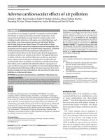
Secondary Acidification

31
used with the reference latitude/longitude being 37°N/123°E (the model domain is not
shown as it is not very different from that shown in Figure 4). The simulation was
conducted for March 2006. In spring in East Asia, considerable long-range transport occurs
because cyclones and anti-cyclones propagating eastward carry contaminated air masses by
turn in cycles of about 5 days.

RUN CNTRL S2 S2NHh Sh ShNH2
SO
2
emission 1 2 2 0.5 0.5
NO
x
emission 1 1 1 1 1
NH
3
emission 1 1 0.5 1 2
Table 5. Ratios of emissions to that of CNTRL run used for sensitivity studies to evaluate
secondary acidification due to future emission changes.
Figure 8 illustrates the simulated (CNTRL) spatial distributions of the SO
2
and NO
x

emission fluxes and monthly mean surface concentrations of SO
4
2-
and t-NO

3
in March 2006.
SO
2
and NO
x
emissions peaks are seen in large emission source regions, and SO
4
2-
and t-NO
3

are transported widely to southward and eastward downwind regions.


Fig. 8. The simulated (CNTRL) spatial distributions of (a) the SO
2
emission flux (μg m
-2
s
-1
),
(b) the NO
x
emission flux (μg m
-2
s
-1
), (c) the monthly mean surface sulfate concentration (μg
m

-3
), and (d) the monthly mean surface total (gas + aerosol) nitrate concentration (μg m
-3
) in
March 2006.
Figure 9 illustrates the simulated (CNTRL) spatial distributions of the gas phase fraction of
nitrate, the monthly accumulated precipitation, and the monthly accumulated dry and wet
deposition of t-NO
3
. The gas phase fraction is larger over the ocean (20–40%) than over the
continent (1–30%) because the surface temperature is higher over the ocean in spring. Also
because of temperature differences, the gas phase fraction over the land is larger in the south

Monitoring, Control and Effects of Air Pollution

32
(5–30%) than in the north (1–5%). The monthly mean surface temperature over the ocean
ranges over about 5–20 °C, whereas it ranges from –20 to 0 °C over the northern continent, and
from 0 to 15 °C over the southern continent (not shown). In general, the dry deposition amount
and the surface concentration are expected to correlate with each other given a relatively
constant dry deposition rate. However, the dry deposition amounts are larger over the
southern edge of the continent and western Japan, whereas the surface concentrations are
larger over the North China Plain, the Sichuan Basin, and the Yangtze Plain. The horizontal
distribution of the dry deposition is rather similar to that of the gas phase fraction, because the
modeled dry deposition velocities of HNO
3
gas (0.9–2.7 cm s
-1
) are much larger than those of
NO

3
-
aerosols (0.02–0.1 cm s
-1
over the land, 0.2–1 cm s
-1
over the ocean). The wet deposition
amounts are large where both the precipitation and the concentrations are large, and they are
about twice to three times the dry deposition amounts.


Fig. 9. Spatial distributions of (a) the gas phase fraction of nitrate (%), (b) monthly accumulated
precipitation (mm) with surface wind vectors (m s
-1
), (c) monthly dry deposition amount of
nitrate (μg m
-2
mon
-1
), and (d) wet deposition of nitrate (μg m
-2
month) in March 2006.
Figure 10 illustrates the gas phase fraction of nitrate and monthly accumulated total (dry +
wet) deposition of t-NO
3
in the CNTRL run and the deviations from the control in the S2
and the S2NHh runs. Doubling SO
2
emissions causes the gas phase fraction to increase by 1–
6% over southern China and over the ocean (Figure 10c and d). The increase of the gas phase

fraction over northern China is less than 1%, however, because of the low temperatures
there. In general, because the East Asian atmosphere is ammonia-rich and is sodium-rich
over the ocean, so the expulsion of NO
3
-
to the gas phase is not very significant. However,
gas phase fraction, of as large as 20% over northern China, is seen, because the counterpart
of NO
3
-
is decreased substantially. As a result of the increase in the gas phase fraction, the
total deposition of nitrate increases by about 5–20 mg m
-2
, corresponding to about 10% of
the total deposition in CNTRL (50–300 mg m
-2
), when SO
2
emissions double. The increase is
larger than 20 mg m
-2
over wide areas when NH
3
emission is halved, accounting for as
much as 50% of the total nitrate of the CNTRL.

Secondary Acidification

33

Fig. 10. Spatial distributions of (left panels) gas phase fraction of nitrate (%) and (right
panels) total (dry plus wet) deposition of nitrate (μg m
-2
mon
-1
). The top panels show the
when NH
3
emissions are halved (bottom panels), a pronounced increase in the CNTRL run
results and the middle and bottom panels show the results for the differences between the
S2 and CNTRL runs (middle) and between the S2NHh and CNTRL runs (bottom).
In contrast, wet plus dry deposition decreases over the Pacific Ocean east of the Japan
archipelago by about 1–10 mg m
-2
in the S2NHh run, probably because the increase in
deposition over the downwind regions (the continent and the ocean close to the continent)
causes the concentration over the regions further downwind to decrease. Consequently,
nitrate deposition also decreases in the regions further downwind.
As discussed before in Sections 3.1 and 3.2, the wet deposition efficiencies of HNO
3
gas and
NO
3
-
aerosol cannot be directly compared with each other because NO
3
-
aerosol particles can
act effectively as CCN. When cloud production and NO
3

-
aerosol activation are very
efficient, secondary acidification may not occur. In contrast, when mature clouds are present
and the gravitational fall of rain droplets is dominant, HNO
3
gas is more efficiently captured
by water droplets and secondary acidification may occur. The RAQM2 model can show the

Monitoring, Control and Effects of Air Pollution

34
quantitative results of secondary acidification due to wet deposition, and the simulation
results should not differ much from reality because the model results for the concentrations
of inorganic components in the air as well as for precipitation have been evaluated
extensively with measurement data. However, in the current off-line coupled WRF-RAQM2
framework, processes related to wet deposition, such as aerosol activation, cloud dynamics,
and cloud microphysics, are based on many assumptions and various parameterizations.
Thus, it is still not possible to determine whether wet scavenging of HNO
3
gas or of NO
3
-

aerosol is in reality more efficient.
4.2.3 Adverse effects of an SO
2
emission decrease: a decrease in nitrate deposition
downwind may cause an increase in deposition even further downwind
The widespread installation of flue-gas desulfurization (FGD) devices is expected to
decrease Asian SO

2
emissions in the future. In China, FGD devices are now being installed
in many coal-fired power plants. From 2001 to 2006, FGD penetration increased from 3% to
30%, causing a 15% decrease in the average SO
2
emission factor of coal-fired power plants
(Zhang et al., 2009).


Fig. 11. Spatial distributions of the differences in the gas phase fraction of nitrate (%) (left
panels) and total (dry + wet) deposition of nitrate (μg m
-2
mon
-1
) (right panels). The upper and
lower panels show the results for (Sh – CNTRL) and the (S2NHh – CNTRL) runs, respectively.
As a result of future SO
2
emission decreases, less secondary acidification should occur.
However, a decrease in nitrate deposition downwind will also mean that t-NO
3
will be
transported longer distances, which may result in increased deposition of t-NO
3
in regions
further downwind.
Figure 11 shows changes in the gas phase fraction of nitrate and in total deposition when
SO
2
emissions are decreased by half. Both the gas phase fraction of nitrate and total nitrate

deposition in downwind regions decrease, by 1–5% and 1–20 mg m
-2
, respectively (upper

Secondary Acidification

35
panels). When NH
3
, the counterpart of NO
3
-
in aerosols, is doubled and SO
2
emissions are
halved, the gas phase fraction of nitrate decreases substantially over downwind regions,
which results in a significant decrease in total nitrate deposition (20–50 mg m
-2
). In the Sh
run, the surface mean t-NO
3
concentration over Pacific coastal regions of Japan increases by
0.5–2% (not shown) and the increase in the total deposition is about 1–5 mg m
-2
over the
same regions (Figure 11b), although the increase is small compared to the total deposition
(100–400 mg m
-2
, Figure 10b).
5. Conclusion

We studied secondary acidification, which is enhanced deposition of NO
3
-
caused by an
increase in the SO
4
2-
concentration, using field observation data as well as numerical
simulations of a volcanic eruption event and the long-range transport of air pollutants.
Because the vapor pressure of H
2
SO
4
gas is extremely low, increased SO
4
2-
expels NO
3
-
in the
aerosol phase to the gas phase, resulting in an increase in the HNO
3
gas fraction. As wet and
dry deposition rates of HNO
3
gas are considered to be more efficient than those of NO
3
-

aerosols, the deposition of total nitrate (HNO

3
gas plus NO
3
-
aerosols) is consequently
enhanced, even though its total concentration remains unchanged.
Secondary acidification was prominent when the Miyakejima Volcano (180 km south of
Tokyo) erupted, emitting a huge amount of SO
2
(9 Tg yr
-1
) into the lower atmosphere (~2000 m
ASL). At the Happo Ridge observatory (1850 m ASL, 300 km north of the volcano), the fraction
of gaseous HNO
3
increased from 40% before the eruption to 95% after the eruption, and the
bimonthly mean NO
3
-
concentration in precipitation increased by 2.7 times after the eruption.
The numerical simulation using the RAQM2 model predicted that as a result of the volcanic
SO
2
emissions, the SO
4
2-
concentration would double and the gas phase fraction of t-NO
3

would increase from 20–40% to 22–45% per month on average over central Japan, which is

downwind of Miyakejima volcano. The increase of dry and wet deposition due to the volcanic
emission was about 0.5–3 and 5–10 (mg m
-2
mon
-1
), respectively. Wet deposition was
decreased in some regions, probably because CCN activation and cloud droplet formation of
NO
3
-
aerosols is more efficient than dissolution of HNO
3
gas into water droplets.
At the Japanese EANET monitoring station at Oki, we found positive correlations between
the following observational parameters:
1.
SO
4
2-
concentration in atmosphere and gas phase fraction of HNO
3

2.
The gas phase fraction of HNO
3
and wet deposition rate of total nitrate
3.
A long-range transport indicator and the wet deposition rate of total nitrate
These positive correlations indicate that secondary acidification occurs during the long-
range transport of air pollutants from the Asian continent to Japan. Secondary acidification

is less efficient in the presence of abundant sea-salt particles, because the contained Na
+

reacts with nitrate to form NaNO
3
, keeping it in the aerosol phase.
We also simulated secondary acidification due to future anthropogenic SO
2
emission
changes using the RAQM2 model. If SO
2
emissions double, the gas phase fraction increases
1–6% over southern China and over the ocean, resulting in an increase of about 10% in total
nitrate deposition over the region. The Asian atmosphere is generally ammonia-rich, so the
expulsion of NO
3
-
to the gas phase is not significant. However, if emission of NH
3
, as the
counterpart of NO
3
-
, is decreased by half, along with the doubling of SO
2
emissions, then the
expulsion of NO
3
-
is significant and total nitrate deposition over the downwind region

increases by as much as 50%. Asian SO
2
emissions are likely to decrease in the future
because of the installation of flue-gas desulfurization devices and petroleum refineries. As
SO
2
emissions decrease, nitrate deposition may also decrease in downwind regions. On the

Monitoring, Control and Effects of Air Pollution

36
other hand, the decrease in nitrate deposition in downwind regions means that total nitrate
will be transported greater distances to regions further downwind.
Our results also indicate that to simulate the concentrations and depositions of t-NO
3

accurately, accurate estimations of emission inventories of SO
2
and NH
3
and of its precursor
NO
x
are important.
Simulated dry deposition velocities and wet scavenging rates include substantial errors and
uncertainties in most numerical models, because those parameters are quite difficult to
evaluate from observational data. Therefore, as simulation techniques become more
advanced, we should revisit this issue again to update our knowledge about what really
happens in the atmosphere.
6. Acknowledgment

We thank Dr. Hikaru Satsumabayashi of Nagano Environmental Conservation Research
Institute, Japan, for providing measurement data from Happo Ridge and for engaging in
meaningful analysis and discussions.
7. References
Abdul-Razzak, H. & Ghan, S. J. (2000). A parameterization of aerosol activation: 2. Multiple
aerosol types, J. Geophys. Res., 105, pp.6837-6844, doi:10.1029/1999JD901161.
Adams, P. J.; Seinfeld, J. H.; Koch, D.; Mickley, L. & Jacob, D. (2001). General circulation
model assessment of direct radiative forcing by the sulfate-nitrate-ammonium-
water inorganic aerosol system. J. Geophys. Res., Vol. 106, No. D1, pp. 1097-1111.
Andreas, R. J. & Kasgnoc, A. D. (1998). A time-averaged inventory of subaerial volcanic
sulfur emission. J. Geophys. Res., Vol.103, No.D19, pp.25,251-25,261.
Brook, J. R.; Di-Giovanni, F.; Cakmak, S., & Meyers, T. P. (1997). Estimation of dry
deposition velocity using inferential models and site-specific meteorology –
Uncertainty due to siting of meteorological towers. Atmos. Environ., Vol. 31, No. 23,
pp. 3911-3919
Clarke, L.; Edmonds, J.; Jacoby, H.; Pitcher, H.; Reilly, J. & Richels, R. (2007). Scenarios of
greenhouse gas emissions and atmospheric concentrations. Sub-report 2.1A of
Synthesis and Assessment Product 2.1 by the U.S. Climate Change Science Program
and the Subcommittee on Global Change Research. Department of Energy, Office
of Biological & Environmental Research, Washington, 7 DC., USA, 154 pp.
Deushi, M. & Shibata, K. (2011). Development of an MRI Chemistry-Climate Model ver.2 for
the study of tropospheric and stratospheric chemistry, Papers in Meteor. Geophys., in
press.
Fujino, J.; Matsui, S.; Matsuoka, Y. & Kainuma, M. (2002). AIM/Trend: Policy Interface,
Climate Policy Assessment, Eds. M. Kainuma, Y. Matsuoka and T. Morita,
Springer, pp.217-232.
Fujino, J.; Nair, R.; Kainuma, M.; Masui, T. & Matsuoka, Y. (2006). Multi-gas mitigation
analysis on stabilization scenarios using AIM global model. Multigas Mitigation
and Climate Policy. The Energy Journal Special Issue.
Hayami, H.; Sakurai, T.; Han, Z.; Ueda, H.; Carmichael, G.; Streets, D.; Holloway, T.; Wang,

Z.; Thongboonchoo, N.; Engardt, M.; Bennet, C.; Fung, C.; Chang, A.; Park, S. U.;
Kajino, M.; Sartelet, K.; Matsuda, K. & Amann, M. (2008). MICS-Asia II: Model
intercomparison and evaluation of particulate sulfate, nitrate and ammonium.
Atmos. Environ., Vol.42, pp.3510-3527.

Secondary Acidification

37
Hijioka, Y.; Matsuoka, Y.; Nishimoto, H.; Masui, M. & Kainuma, M. (2008). Global GHG
emissions scenarios under GHG concentration stabilization targets. J. Global
Environ. Eng., Vol.13, pp.97-108.
Intergovernmental Panel on Climate Change (2000), Special Report on Emissions Scenarios,
edited by N. Nakicenovic, 599 pp., Cambridge Univ. Press., New York.
Jylhä, K. (1999a). Relationship between the scavenging coefficient for pollutants in
precipitation and the radar reflectivity factor. Part I: derivation. J. Appl. Meteorol.,
Vol. 38, pp. 1421-1434
Jylhä, K. (1999b). Relationship between the scavenging coefficient for pollutants in
precipitation and the radar reflectivity factor. Part II: Applications. J. Appl.
Meteorol., Vol. 38, pp. 1435-1447.
Kajino, M. (2011). MADMS : Modal Aerosol Dynamics model for multiple Modes and fractal
Shapes in the free-molecular and near-continuum regimes. J. Aerosol Sci., Vol. 42,
No. 4, pp.224-248.
Kajino, M . & Kondo, Y. (2011). EMTACS : Development and regional-scale simulation of a
size, chemical, mixing type, and soot shape resolved atmospheric particle model. J.
Geophys. Res., Vol. 116, D02303, doi :10.1029/2010JD015030
Kajino, M. & Ueda, H. (2007). Increase in nitrate deposition as a result of sulfur dioxide
emission increase in Asia: indirect acidification. Air Pollution Modeling and its
Application XVIII., Eds. C. Borrego, E. Renner, Elsevier, ISBN:978-0-444-52987-9, pp.
134-143
Kajino, M.; Ueda, H. ; Satsumabayashi, H ; & An, J. (2004). Impacts of the eruption of

Miyakejima Volcano on air quality over far east Asia. J. Geophys. Res., Vol. 109,
D21204, doi:10.1029/2004JD004762
Kajino, M.; Ueda, H. ; Satsumabayashi, H ; & Han, Z. (2005). Increase in nitrate and chloride
deposition in east Asia due to increased sulfate associated with the eruption of
Miyakejima Volcano. J. Geophys. Res., Vol. 110, D18203, doi:10.1029/2005JD005879
Kajino, M ; Ueda, H. & Nakayama, S. (2008). Secondary acidification : Changes in gas-
aerosol partitioning of semivolatile nitric acid and enhancement of its deposition
due to increased emission and concentration of SOx. J. Geophys. Res., Vol.113,
D03302, doi:1029/2007JD008635
Kajino, M.; Ueda, H.; Sato, K. & Sakurai, T. (2010). Spatial distribution of the source-receptor
relationship of sulfur in Northeast Asia. Atmos. Chem. Phys. Discuss., Vol.10,
pp.30,089-30,127.
Kazahaya, K. (2001). Amount of volcanic gases erupted by Miyakejima Volcano, in
Miyakejima Island Eruption and Wide Area Air Pollution (in Japanese), Jpn. Soc. For
Atmos. Environ., pp. 17-26.
Kim, Y. P.; Seinfeld, J. H. & Saxena, P. (1993). Atmospheric gas-aerosol equilibrium: I.
Thermodynamic model, Aerosol Sci. Technol., Vol.19, pp.157-181.
Klimont, Z.; Cofala, J.; Schopp, W.; Amann, M.; Streets, D. G.; Ichikawa, Y. & Fujita, S.
(2001). Projections of SO
2
, NO
x
, NH
3
and VOC emissions in East Asia up to 2030,
Water Air Soil Pollut., Vol. 130, pp.193-198.
Kurokawa, J.; Ohara, T.; Uno, I.; Hayasaka, M. & Tanimoto, H. (2009). Influence of
meteorological variability on interannual variations of springtime boundary layer
ozone over Japan during 1981-2005. Atmos. Chem. Phys., Vol. 9, pp.6287-6304.
Lee, S.; Ghim, Y. S.; Kim, Y. P. & Kim, J. Y. (2006). Estimation of the seasonal variation of

particulate nitrate and sensitivity to the emission changes in the greater Seoul area.
Atmos. Environ., Vol. 40, pp. 3724-3736.

Monitoring, Control and Effects of Air Pollution

38
Meng, Z.; Seinfeld, J. H.; Saxena, P.; Kim, Y. P. (1995). Atmospheric gas-aerosol equilibrium:
IV. Thermodynamics of carbonates, Aerosol Sci. Technol., Vol.22, pp.131-154
Morino, Y.; Kondo, Y.; Takegawa, N.; Miyaazaki, Y.; Kita, K.; Komazaki, Y.; Fukuda, M.;
Miyakawa, T.; Moteki, N. & Worsnop, D. R. (2006). Partitioning of HNO3 and
particulate nitrate over Tokyo: Effects of vertical mixing. J. Geophys. Res., Vol. 111,
D15215, doi:10.1029/2005JD006887
Moya, M.; Ansari, A. S. & Pandis, S. N. (2001). Partitioning of nitrate and ammonium
between the gas and particulate phases during the 1997 IMADA-AVER study in
Mexico City. Atmos. Environ., Vol. 35, pp. 1791-1804.
Nemitz, E. & Sutton, M. A. (2004). Gas-particle interactions above a Dutch heathland: III.
Modeling the influence of the NH
3
-HNO
3
-NH
4
NO
3
equilibrium on size-segregated
particle fluxes. Atmos. Chem. Phys., Vol. 4, pp. 1025-1045.
Ohara, T.; Akimoto, H.; Kurokawa, J.; Horii, J.; Yamaji, K.; Yan, X. & Hayasaka, T. (2007). An
Asian emission inventory of anthropogenic emission sources for the period 1980-
2020. Atmos. Chem. Phys. Vol. 7, pp. 4419-4444.
Riahi, K.; Gruebler, A. & Nakicenovic, N. (2007). Scenarios of long-term socio-economic and

environmental development under climate stabilization. Technological Forecasting
and Social Change, Vol. 74, No. 7, pp.887-935.
Satsumabayashi, H.; Kawamura, M.; Katsuno, T.; Futaki, K.; Murano, K.; Carmichael, G. R.;
Kajino, M.; Horiguchi, M. & Ueda, H. (2004). Effects of Miyake volcanic effluents on
airborne particles and precipitation in central Japan. J. Geophys. Res., Vol. 109,
D19202, doi: 1029/2003JD004204
Schaap, M.; van Loon, M.; ten Brink, H. M.; Dentener, F. J. & Builtjes, P. J. H. (2004).
Secondary inorganic aerosol simulations for Europe with special attention to
nitrate. Atmos. Chem. Phys., Vol. 4, pp. 857-874
Seinfeld, J. H. & Pandis, S. N. (2006). Atmospheric Chemistry and Physics: From Air Pollution to
Climate Change, second edition, Wiley Interscience, New York.
Skamarock, W. C.; Klemp, J. B.; Dudhia, J.; Gill, D. O.; Barker, D. M.; Duda, M. G.; Huang, X.
Y.; Wang, W. & Powers, J. G. (2008). A description of the advanced research WRF
version 3, Tech. Note, NCAR/TN~475+STR, 125 pp. Natl. Cent. Atmos. Res., Boulder,
Colo.
Streets, D. G.; Bond, T. C.; Carmichael, G. R.; Fernandes, S. D.; Fu, Q.; He, D.; Klimont, Z.;
Nelson, S. M.; Tsai, N. Y.; Wang, M. Q.; Woo, J H. & Yarber, K. F. (2003). An
inventory of gaseous and primary aerosol emissions in Asia in the year 2000. J.
Geophys. Res., Vol.108, No.D21, 8809, doi:10.1029/2002JD003093.
van Vuuren, D. P.; den Elzen, M. G. J.; Lucas, P. L.; Eickhout, B.; Strengers, B. J.; van Ruijven,
B.; Wonink, S.; van Houdt, R. (2007) Stabilizing greenhouse gas concentrations at
low levels: an assessment of reduction strategies and costs. Climate Change, 81,
pp.119-159.
Zhang, Q.; Streets, D. G.; Carmichael, G. R.; He, K. B.; Huo, H.; Kannari, A.; Klimont, Z.;
Partk, I. S.; Reddy, S.; Fu, J. S.; Chen, D.; Duan, L.; Lei, Y.; Wang, L. T. & Yao, Z. L.
(2009). Asian emissions in 2006 for the NASA INTEX-B mission. Atmos. Chem. Phys.,
Vol. 9, pp.5131-5153.
Part 2
Air Pollution Monitoring and Modelling

3
Gas Sensors for Monitoring Air Pollution
Kwang Soo Yoo
Department of Materials Science and Engineering, University of Seoul,
Korea
1. Introduction
The air pollution caused by exhaust gases from automobiles has become a critical issue. In
some regions, fossil fuel combustion is a problem as well. The principal gases that cause air
pollution from automobiles are nitrogen oxides, NO
x
(NO and NO
2
), and carbon monoxide
(CO). Because NO
x
gases with sulfur oxides (SO
x
) emitted from coal fired plants cause acid

rain and global warming and produce ozone (O
3
) that leads to serious metropolitan smog
from photochemical reaction, they must be detected and reduced [1-5].
In addition, as greater amounts of oil organic compounds are currently being produced by
applied construction materials and households, the number of people who develop various
symptoms after moving into a new apartment (e.g., tickle, vertigo, headache, skin trouble) is
increasing [6,7]. The principal gases that cause this phenomenon (called “sick-building
syndrome”) are formaldehyde (HCHO) and volatile organic compounds (VOCs) [8].
Especially, formaldehyde is the most dangerous among indoor pollutants as it could harm
all kinds of organisms. Considering these, the allowed concentration of formaldehyde in the
Netherlands and Germany is only 0.1 ppm [9,10]. Therefore, gas sensors with excellent
reactivity and stability are needed.
The first decade of the 21
st
century has been labeled by some as the “Sensor Decade.” A sensor
is a device that converts a physical phenomenon into an electrical signal. As such, sensors
represent part of the interface between the physical world and the world of electrical devices,
such as computers. In recent years, sensors have received people’s attention as one of the
important devices in electronic systems and enormous capability for information processing
has been developed within the electronics industry. Of all sensors, gas sensors and light
sensors have been most actively studied [11-13]. The final goal of gas sensor development is to
establish the array technology of multifunctional gas sensors that can monitor air pollution
with low cost, and is to fabricate the electronic nose using this technology.
Gas sensors are defined as a device that can substitute for human olfaction, and there are
many researches being conducted to monitor air pollution by using these gas sensors. Gas
sensors can be classified into semiconductor-type, solid electrolyte-type, electrochemical-
type and catalytic combustion-type. Among these, the semiconductor-type gas sensor, the
most well-known, is operated by changing its conductivity when it is exposed to gas. The
semiconductor-type gas sensor has the advantages of rapid reactivity, efficiency, and gas

selectivity when suitable additives are applied to it [14,15]. Sensors made of inorganic
materials are the most commonly used, especially ceramics. One reason is that many sensors
are used in very severe conditions such as high temperature, reactive or corrosive
atmosphere and high humidity, and ceramics are most reliable materials in these conditions.
Another reason may be that the microstructure of ceramics can be controlled by process

Monitoring, Control and Effects of Air Pollution

42
conditions. In general, electrical, mechanical and optical properties of a material are
controlled by changing its composition. In ceramics, however, these properties are also
controlled by changing its microstructure [13]. The gas-sensing materials for semiconductor-
type are SnO
2
, WO
3
, In
2
O
3
, perovskite-structure oxides, etc., and the electrolyte for solid
electrolyte-type gas sensor is Na
3
Zr
2
Si
2
PO
12
[1,2,4,16-19].

In this chapter, pollutants and sources of air pollution are briefly explained. Then
environmental gas sensors for monitoring air pollution are introduced systematically and
the fabrication methods and characteristics of each gas sensor are explained at length with
recent research trends.
2. Air pollution [20]
Air pollution is the introduction of chemicals, particulate matter, or biological materials that
cause harm or discomfort to humans or other living organisms, or cause damage to the
natural environment or built environment, into the atmosphere. The atmosphere is a
complex dynamic natural gaseous system that is essential to support life on planet Earth.
Stratospheric ozone layer depletion due to air pollution has been recognized as a threat to
human health as well as to the Earth's ecosystems. Indoor air pollution and urban air quality
are listed as two of the world's worst pollution problems in the 2008 Blacksmith Institute
World's Worst Polluted Places report [21].
2.1 Pollutants
A substance in the air that can cause harm to humans and to the environment is known as an
air pollutant. Pollutants can be in the form of solid particles, liquid droplets, or gases. They
may be natural or man-made [22]. Pollutants can be classified as primary or secondary.
Usually, primary pollutants are directly emitted from a process, such as ashes from a volcanic
eruption, the NO
x
and CO gases from a motor vehicle exhaust or SO
x
released from factories.
Secondary pollutants are not emitted directly. Rather, they form in the air when primary
pollutants react or interact. An important example of a secondary pollutant is ground level
ozone - one of the many secondary pollutants that make up photochemical smog. Some
pollutants may be both primary and secondary: that is, they are both emitted directly and
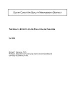
formed from other primary pollutants. Causes and effects of air pollution are shown in Fig. 1.

Fig. 1. Schematic drawing, causes and effects of air pollution: (1) greenhouse effect, (2)
particulate contamination, (3) increased UV radiation, (4) acid rain, (5) increased ground
level ozone concentration, (6) increased levels of nitrogen oxides [20].

Gas Sensors for Monitoring Air Pollution

43
2.1.1 Major primary pollutants
• Nitrogen oxides (NO
x
): especially nitrogen dioxide (NO
2
). NO
2
is emitted from high
temperature combustion. Can be seen as the brown haze dome above or plume
downwind of cities. This reddish-brown toxic gas has a characteristic sharp, biting
odor. NO
2
is one of the most prominent air pollutants.
• Carbon monoxide (CO): CO is a colorless, odorless, non-irritating but very poisonous
gas. It is a product by incomplete combustion of fuel such as natural gas, coal or wood.
Vehicular exhaust is a major source of carbon monoxide.
• Carbon dioxide (CO
2
): CO
2
is a colorless, odorless, non-toxic greenhouse gas associated
with ocean acidification, emitted from sources such as combustion, cement production,
and respiration.

• Volatile organic compounds (VOCs): VOCs are an important outdoor air pollutant. In
this field they are often divided into the separate categories of methane (CH
4
) and non-
methane (NMVOCs). CH4 is an extremely efficient greenhouse gas which enhances
global warming. Other hydrocarbon VOCs are also significant greenhouse gases via
their role in creating ozone and in prolonging the life of CH
4
in the atmosphere,
although the effect varies depending on local air quality. Within the NMVOCs, the
aromatic compounds such as benzene, toluene and xylene are suspected carcinogens
and may lead to leukemia through prolonged exposure. 1,3-butadiene is another
dangerous compound which is often associated with industrial uses.
• Formaldehyde (HCHO): HCHO is the most dangerous among the indoor pollutants as
it could harm all kinds of organisms. As great amounts of oil organic compounds are
induced by applied construction materials and households, HCHO and VOCs are
produced and cause various symptoms (called “sick-building syndrome”) after moving
into a new apartment [6-8].
• Ammonia (NH
3
): NH
3
is emitted from agricultural processes. It is normally
encountered as a gas with a characteristic pungent odor. NH
3
contributes significantly
to the nutritional needs of terrestrial organisms by serving as a precursor to foodstuffs
and fertilizers. NH
3
, either directly or indirectly, is also a building block for the

synthesis of many pharmaceuticals. Although in wide use, NH
3
is both caustic and
hazardous.
• Sulfur oxides (SO
x
): especially sulphur dioxide (SO
2
). SO
2
is produced by volcanoes and
in various industrial processes. Since coal and petroleum often contain sulphur
compounds, their combustion generates SO
2
. Further oxidation of SO
2
, usually in the
presence of a catalyst such as NO
2
, forms H
2
SO
4
, and thus acid rain. This is one of the
causes for concern over the environmental impact of the use of these fuels as power
sources.
• Particulate matter (PM): Particulates, alternatively referred to as PM or fine particles,
are tiny particles of solid or liquid suspended in a gas. In contrast, aerosol refers to
particles and the gas together. Some particulates occur naturally, originating from
volcanoes, dust storms, forest and grassland fires, living vegetation, and sea spray.

Human activities, such as the burning of fossil fuels in vehicles, power plants and
various industrial processes also generate significant amounts of aerosols. Averaged
over the globe, anthropogenic aerosols - those made by human activities - currently
account for about 10 percents of the total amount of aerosols in our atmosphere.

Monitoring, Control and Effects of Air Pollution

44
Increased levels of fine particles in the air are linked to health hazards such as heart
disease [23], altered lung function and lung cancer.
• Chlorofluorocarbons (CFCs): CFCs are harmful to the ozone layer emitted from
products currently banned from use [24,25].
• Persistent free radicals connected to airborne fine particles could cause
cardiopulmonary disease.
• Toxic metals, such as lead, cadmium and copper
• Odors such as from garbage, sewage, and industrial processes
• Radioactive pollutants produced by nuclear explosions, war explosives, and natural
processes such as the radioactive decay of uranium.
2.1.2 Secondary pollutants
• PM formed from gaseous primary pollutants and compounds in photochemical smog:
Smog is a kind of air pollution and the word "smog" means a portmanteau of smoke
and fog. Classic smog (London type smog) results from large amounts of coal burning
in an area caused by a mixture of smoke and sulfur dioxide. Modern smog
(photochemical or Los Angeles type smog) does not usually come from coal but from
vehicular and industrial emissions that are acted on in the atmosphere by ultraviolet
light from the sun to form secondary pollutants that also combine with the primary
emissions to form photochemical smog.
• Ground level ozone (O
3
) formed from NO

x
and VOCs: O
3
is a key constituent of the
troposphere. It is also an important constituent of certain regions of the stratosphere
commonly known as the Ozone layer. Photochemical and chemical reactions involving
it drive many of the chemical processes that occur in the atmosphere by day and by
night. At abnormally high concentrations brought about by human activities (largely
the combustion of fossil fuel), it is a pollutant, and a constituent of smog.
• Peroxyacetyl nitrate (PAN) similarly formed from NO
x
and VOCs.
2.2 Sources
Sources of air pollution refer to the various locations, activities or factors which are
responsible for the releasing of pollutants into the atmosphere. These sources can be
classified into two major categories.
2.2.1 Anthropogenic sources (human activity)
• "Stationary Sources" include smoke stacks of power plants, manufacturing facilities
(factories) and waste incinerators, as well as furnaces and other types of fuel-burning
heating devices.
• "Mobile Sources" include motor vehicles, marine vessels, aircraft and the effect of sound
etc.
• Chemicals, dust and controlled burn practices in agriculture and forestry management.
Controlled or prescribed burning is a technique sometimes used in forest management,
farming, prairie restoration or greenhouse gas abatement. Fire is a natural part of both
forest and grassland ecology and controlled fire can be a tool for foresters. Controlled
burning stimulates the germination of some desirable forest trees, thus renewing the
forest.

Gas Sensors for Monitoring Air Pollution

45
• Fumes from paint, hair spray, varnish, aerosol sprays and other solvents.
• Waste deposition in landfills, which generate methane. Methane is not toxic; however, it
is highly flammable and may form explosive mixtures with air. Methane is also an
asphyxiant and may displace oxygen in an enclosed space. Asphyxia or suffocation may
result if the oxygen concentration is reduced to below 19.5% by displacement.
• Military, such as nuclear weapons, toxic gases, germ warfare and rocketry.
2.2.2 Natural sources
• Dust from natural sources, usually large areas of land with little or no vegetation.
• CH
4
gas emitted by the digestion of food by animals, for example, cattle.
• Radon gas from radioactive decay within the Earth's crust. Radon is a colorless,
odorless, naturally occurring, radioactive noble gas that is formed from the decay of
radium. It is considered to be a health hazard. Radon gas from natural sources can
accumulate in buildings, especially in confined areas such as the basement and it is the
second most frequent cause of lung cancer, after cigarette smoking.
• Smoke and CO from wildfires.
• Vegetation, in some regions, emits environmentally significant amounts of VOCs on
warmer days. These VOCs react with primary anthropogenic pollutants - specifically,
NO
x
, SO
2
, and anthropogenic organic carbon compounds - to produce a seasonal haze
of secondary pollutants [26].
• Volcanic activity, which produce sulfur, chlorine, and ash particulates.
3. Environmental gas sensors
A broad definition of environmental monitoring would include all aspects of air and water

quality, soil contamination, electromagnetic radiation, noise, even heat release and light
source pollution. However, the major environmental gas sensors are to monitor pollution in
air, water, and soil as shown in Table 1 [27]. Environmental standard concentration and
threshold limit value for six important gases of air pollution are listed in Table 2 [28,29].
Some information about gas sensors on the base of most familiar metal oxides and
technological peculiarities of these sensors fabrication, which can be used for such selection,
is presented in Tables 3 and 4 [30]. Gas sensors for monitoring principal gases among air
pollutants are described in detail by using typical examples here.

Fixed monitors Mobile monitors

Stationary source Ambient Portable Personal
Air
Industrial
emissions, Leaks,
Car exhausts,
Biochemicals
Air quality Air quality, Surveys Gas alarms
Water
Drinking water,
Effluent
Water
pollution,
Intake
monitoring
Water pollution,
Pollution tracing
Drinking
water
Land Waste disposal Remediation, Leaks

Table 1. Classification of Environmental Monitoring Applications [27]

Monitoring, Control and Effects of Air Pollution

46
Concentration
Pollutants
Environmental TLV* Request of sensors
Ref.
NO
x
Below 0.04-0.06 ppm (daily average)
NO
2
: 3 ppm,
NO: 25 ppm
0.01-0.3 ppm
28

CO
2
- 5000 ppm 200-400 ppm 28
CO 35 ppm
†
(1 h average) 50 ppm 0.1-10 ppm 28,
†
29
HCHO - 1 ppm - 29
SO
2

Below 0.04 ppm (daily average) 2 ppm 0-2 ppm 28
NH
3
- 25 ppm - 28
O
3
Below 0.06 ppm (1 h average) 0.1 ppm 0-0.5 ppm 28
CFC** - - 20 ppt 28
*TLV: maximum exposure in 8 h period in 40 h work week
**CFC: Chlorofluorocarbon (Freon)
Table 2. Environmental Standard Concentration and Threshold Limit Value (TLV) of Air
Pollution

Materials Advantages Disadvantages
SnO
2

High sensitivity, Good stability in
reducing atmosphere
Low selectivity, Dependence on air
humidity
WO
3

Good sensitivity to oxidizing
gases, Good thermal stability
Low sensitivity to reducing gases,
Dependence on air humidity, Slow
recovery process
Ga

2
O
3

High stability, Possibility to
operate at high temperatures
Low selectivity, Average sensitivity
In
2
O
3

High sensitivity to oxidizing
gases, Fast response and recovery,
Low sensitivity to air humidity
Low stability at low oxygen partial
pressure
CTO
(CrTiO
x
)
High stability, Low sensitivity to
air humidity
Average sensitivity

Table 3. Main Advantages and Disadvantages of Well-known Metal Oxides for Gas Sensor
Applications [30]

Metal
oxides

Detection gases Operating
temperature (ºC)
Stability Compatibility with
IC fabrication
SnO
2
Reducing gases
(CO, H
2
, CH
4
, etc.)
200-400 Excellent Imperfect
WO
3
NO
x
, O
3
, H
2
S, SO
2
300-500 Excellent Low
Ga
2
O
3
O
2

, CO 600-900 High Good
In
2
O
3
O
3
, NO
x
200-400 Moderate Good
MoO
3
NH
3
, NO
2
200-450 Moderate Moderate
TiO
2
O
2
, CO, SO
2
350-800 Enhanced Moderate
ZnO CH
4
, C
4
H
10

, O
3
, NO
x
250-350 Satisfactory Good
CTO H
2
S, NH
3
, CO, volatile
organic compounds
300-450 High Imperfect
Fe
2
O
3
Alcohol, CH
4
, NO
2
250-450 Low Moderate
Table 4. Operating Parameters of Solid-state Gas Sensors on the Base of Metal Oxides and
Technological Peculiarities of their Fabrication [30]

Gas Sensors for Monitoring Air Pollution

47
3.1 NO
x
gas sensor

Nitrogen oxide (NO
x
) sensing materials reported by several investigators are WO
3
, ZnO,
SnO
2
, In
2
O
3
, TiO
2
, etc. Among these, WO
3
is known as the most promising NO
x
gas-sensing
material [19,31-39]. These oxides have the advantages of rapid reactivity, efficiency, and gas
selectivity when suitable additives are applied to them.
These sensing materials are oxygen-deficient nonstoichiometric compounds. The
conductivity of these n-type semiconductors, such as WO
3
and In
2
O
3
,

is estimated based on

the electron created by the surplus metal. When sensing materials are exposed to oxidizing
gases at temperature ranging from 200ºC to 300ºC, the concentration of electrons is
decreased due to the reaction between the electron and the gas. Consequently, the
conductivity decreases and the resistance increases.
As NO
x
is also an oxidizing gas, the concentration of electrons is decreased due to the
reaction between the electrons in the sensing materials and NO
x
gas, as shown in the
following equations:

2
2
1
2
2
NO e N O
−−
+⎯⎯→+
(1)

2
2
2NO e NO O
−−
+⎯⎯→+
(2)
Example [19]:
The powders of various gas-sensing materials were prepared using the solid-state reaction

method, starting from the raw materials, WO
3
and In
2
O
3
. To improve the reactivity and
sensitivity of the gas sensors, 0.1-wt% PdCl
2
was added as a catalyst. The powders were
mixed, dried at 50ºC, and then calcined at 1000ºC. Thick-film NO
x
gas sensors were
prepared on alumina substrate. The Pt electrodes were also printed with a silkscreen
method before the deposition of the WO
3
and In
2
O
3
gas-sensing layer. Schematic diagrams
of the sensor are shown in Figure 2. To control the operating temperatures, a printing paste
was used to form a Pt heater at the back of the alumina substrate. Pt wires were used as
conductuve wires and were attached using silver paste.


Fig. 2. Schematic diagrams of the gas sensor [19].

Monitoring, Control and Effects of Air Pollution

48
The gas-sensing properties were measured in a conventional gas-flow apparatus in the
range of 1-5-ppm NO
x
by mixing the parent gas (500-ppm NO
x
in an N
2
balance) and dry
synthetic air. The resistance of the sensor was calculated as:

1
C
sL
RL
V
RR
V
⎛⎞
=−
⎜⎟
⎜⎟
⎝⎠
(3)
where R
s
is the resistance of the sensor, R
L
is the resistance of the load which was
controlled to fix the output voltage to the half of the input voltage because of the change

the resistance of the sensor with the change of temperature. V
C
is the input voltage and
V
RL
is the output voltage. The sensitivity (S), which refers to the resistance of a sensor that
has been exposed to NO
x
gas versus the resistance of a sensor that has been exposed to
air, was calculated as:

g
as
air
R
S
R
⎛⎞
=
⎜⎟
⎜⎟
⎝⎠
(4)
where R
gas
is the resistance of the sensor that has been exposed to NO
x
gas and R
air
is the

resistance of the sensor that has been exposed to air. In the gas mixtures of NO
x
/air, the NO
x

concentration varied from 1 ppm to 5 ppm.
As shown in Figures 3 and 4, when the sensors were exposed to NO
x
gas, their resistance
increased. Below 250ºC the resistance of the WO
3
and In
2
O
3
were very high, so they could
not detect the NO
x
gas as there were hardly the resistance change of the WO
3
and In
2
O
3
.
The highest sensitivities of the In
2
O
3
to NO

x
were at 300ºC, as were the highest
sensitivities of the WO
3
to NO. The highest sensitivities of the WO
3
to NO
2
were at 250ºC,
though.
Comparing the sensing property of In
2
O
3
with that of WO
3
, the sensitivities of In
2
O
3
to NO
were higher than those of WO
3
to NO, although they were similar. The highest sensitivity
(
R
gas
/R
air
) of In

2
O
3
to 5-ppm NO was 10.22 when it was measured at 300ºC.


(a) NO gas (b) NO
2
gas
Fig. 3. NO
x
Gas-sensing properites of WO
3
[19].

Gas Sensors for Monitoring Air Pollution

49

(a) NO gas (b) NO
2
gas
Fig. 4. NO
x
Gas-sensing properites of In
2
O
3
[19].
3.2 CO

2
gas sensor
Carbon dioxide (CO
2
) sensors have been greatly demanded for monitoring or controlling
CO
2
in various fields such as combustion process, biology, farming as well as air pollution.
So far, many kinds of CO
2
sensors using various materials, such as solid electrolyte, mixed
oxide capacitors, polymers with carbonate solution and so on, have been investigated [40-
44]. Among them, solid electrolyte-type CO
2
sensors are of particular interest from the
viewpoint of low-cost, high-sensitivity, high-selectivity and simple-element structure [45].
Most researches concerning the use of NASICON as active element for gas sensors have
been focused on the Na
1+x
Zr
2
Si
x
P
3-x
O
12
formula, in the composition range of 1.8 < x < 2.4,
because in this range, conductivity shows the largest value [46-48]. A commercial NASICON
with a nominal-composition Na

3
Zr
2
Si
2
PO
12
has been investigated as a CO
2
electrochemical
sensor [49,50].
CO
2
sensing properties can be upgraded with auxiliary phases in sensing electrodes, which
are binary carbonate systems such as Na
2
CO
3
-BaCO
3
, Na
2
CO
3
-CaCO
3
, Li
2
CO
3

-BaCO
3
, and
Li
2
CO
3
-CaCO
3
. The binary systems bring about several advantages such as better long-term
stability, quick response time, and resistance to water vapor interruption [18,40,51-54]. The
device improved in this way has much increased feasibility in practice [55].
Example [18]
The NASICON powder was prepared using the sol-gel method, starting from the solutions
of ZrO(NO
3
)
2
·8H
2
O, NH
4
H
2
PO
4
, and Na
2
SiO
3

·9H
2
O. The solutions were mixed together to
form a sol, which was further dehydrated at 80
o
C to form a gel. The gel was then dried at
120ºC for 8 hours to form a fine dry powder, which was then ground and calcined at 750ºC
to eliminate the organic remains. Afterwards, the calcined material was reground.

The NASICON layer was screen-printed with a paste on the alumina substrate. The Pt
electrodes were also screen-printed on the designated regions before and after the
deposition of the NASICON layer. The assembly was sintered at 900
o
C, 1000
o
C, and 1100
o
C
for 4 hours in air, respectively. After this, a series of auxiliary phases (Na
2
CO
3
-CaCO
3
) was
screen-printed on the Pt sensing electrode. The schematic diagram of the sensor is shown in
Figure 5.

Monitoring, Control and Effects of Air Pollution

50

Fig. 5. Schematic diagrams of the CO
2
gas sensor [18].

10
3
10
4
-330
-320
-310
-300
-290
-280
-270
-260
-250
-240
-230
-220
-210
-200
470
o
C, 73.7 mV/decade
420
o
C, 54.3 mV/decade

400
o
C, 43.8 mV/decade


EMF (mv)
CO
2
concentration (ppm)

10
3
10
4
-390
-380
-370
-360
-350
-340
-330
-320
-310
-300
-290
-280
-270
-260
470
o

C, 72.7 mV/decade
420
o
C, 57.3 mV/decade
400
o
C, 46.0 mV/decade


EMF (mv)
CO
2
concentration (ppm)

10
3
10
4
-350
-340
-330
-320
-310
-300
-290
-280
-270
-260
-250
-240

-230
-220
470
o
C, 73.0 mV/decade
420
o
C, 63.3 mV/decade
400
o
C, 49.1 mV/decade

EMF (mv)
CO
2
concentration (ppm)

10
3
10
4
-350
-340
-330
-320
-310
-300
-290
-280
-270

-260
-250
-240
-230
-220
-210
470
o
C, 73.3 mV/decade
420
o
C, 66 mV/decade
400
o
C, 50.2 mV/decade

EMF (mv)
CO
2
concentration (ppm)

Fig. 6. CO
2
concentration vs. EMF for the CO
2
gas sensors attached with (a) Na
2
CO
3
-CaCO

3

= 1:0, (b) Na
2
CO
3
-CaCO
3
= 1:0.5, (c) Na
2
CO
3
-CaCO
3
= 1:1.5, and (d) Na
2
CO
3
-CaCO
3
= 1:2
[18].
(a)
(b)
(d)
(c)