Monitoring Control and Effects of Air Pollution Part 4 pot

Gas Sensors for Monitoring Air Pollution

51
Gas-sensing properties were measured in a conventional gas-flow apparatus by changing
the mixing ratio between the parent gas (4% CO
2
in an N
2
balance) and dry synthetic air.
The operating temperature was controlled by monitoring the applied voltage and current
using the power supply. The sensors were exposed to the flow (100 cm
3
/min) of the
required sample gases. The gas mixtures of CO
2
/air with the CO
2
concentration varied from
1,000 to 10,000 ppm.
Four types of sensors were fabricated from NASICON as a solid electrolyte. A series of
Na
2
CO
3
-CaCO
3
mixtures at the molar ratio range of 1:0-1:2 was attached to the sensing
electrode. Figure 6 shows the EMF response to CO
2
as a function of the CO

2
concentration at
various temperatures. The EMF variation for each sensor at 470
o
C agreed well with the
theoretical value of 74.0 mV/decade, based on a two-electron electrochemical reaction. As
the temperature decreased, however, the slope tended to deviate from the ideal. Quite
noticeably, the deviation could be suppressed very effectively with Na
2
CO
3
-CaCO
3
(1:2),
which allowed 50.2 mV/decade to be kept at temperatures as low as approximately 400
o
C.
An increase in the amount of CaCO
3
at the auxiliary phase is fairly effective for keeping the
theoretical value at lower temperatures, whereas an adverse effect occurred when the
CaCO
3
content was insufficient. The mechanism behind such improvements is not yet well
understood, though. It requires further research.
3.3 HCHO gas sensor
Formaldehyde (HCHO) is an achromatic toxic gas and has a stimulating scent. When
exposed to HCHO gas even just for a short time, a person may develop headache and
vertigo, and when exposed to it for a long time, a person may develop asthma and other
lung diseases. When exposed to high concentrations of HCHO, a person may develop

pneumonia or edema of the lungs [9]. Considering these, the allowed concentrations of
formaldehyde in Korea, Denmark, the Netherlands, and Germany are only 2 ppm, 0.2 ppm,
0.1 ppm, and 0.1 ppm, respectively [10]. Therefore, gas sensors with excellent reactivity and
stability are needed. In view of the above, numerous attempts are being made to reduce the
amount of HCHO in the air. Few studies have been conducted, however, on the detection
and the measurement of the amount of HCHO gas in the air by using ceramic gas sensors.
HCHO sensing materials are perovskite-structure oxides (ABO
3
) as the semiconductor type.
ABO
3
-type materials have the advantage of high stability. The sensitivity and selectivity of
these kinds of sensors can be controlled by selecting suitable A and B atoms or through
chemical doping with A
1-x
A
x
B
1-y
B
y
O
3
materials [56].
La
1-x
Sr
x
FeO
3

ceramics are ABO
3
perovskite materials. They are nonstochiometric compounds
and p-type semiconductors whose conductivity is estimated through the holes created by
the surplus oxygen therein. Substitution at the A-site of an element with a different valence
(
e.g., the replacement of La
3+
by Sr
2+
) leads to the formation of oxygen vacancies and high-
valence cations at the B-site, which results in a significant change in the catalytic activity [57-
60]. When these sensing materials are exposed to reducing gases like CO, CH
4
, and HCHO,
their conductivity decreases, and their resistance increases because of the chemical surface
reactions between the reducing gas and the surplus oxygen [61-63].
Example [17]
La
1-x
Sr
x
FeO
3
powders (x = 0, 0.2, 0.5) were prepared through the conventional solid-state
reaction method, starting from raw materials of La
2
O
3
, SrO, and Fe

2
O
3
. The mixed powders
were dried and were calcined at 1000ºC.

Monitoring, Control and Effects of Air Pollution

52
The La
1-x
Sr
x
FeO
3
sensing layers were silkscreen-printed on the alumina substrate. The Pt
electrodes were also silkscreen-printed on the designated regions before the deposition of
the La
1-x
Sr
x
FeO
3
layer. Schematic diagrams of the sensor are shown in Figure 2.
The gas-sensing properties were measured in a conventional gas-flow apparatus by mixing
the parent gas (10 to 50 ppm HCHO in N
2
balance) and dry synthetic air. The resistance of
the sensor was calculated by using eq. (3). The gas sensitivity, which refers to the resistance
of a sensor that has been exposed to HCHO gas versus the resistance of a sensor that has

been exposed to air, was calculated as eq. (4). To confirm the selectivity of the sensors, the
gas-sensitivities for CO
2
, N
2
, and C
3
H
8
were also measured. The operating temperature was
controlled by monitoring the voltage and current applied by using a power supply. The
sensors were exposed to a flow (200 cm
3
/min) of the required sample gases. Gas mixtures of
HCHO/air with the HCHO concentration varying from 10 ppm to 50 ppm were used.
As HCHO gas is a reducing gas, free electrons are released due to the reaction between the
surplus oxygen in the sensing materials and the gas [62], as shown in the following
equation:

2
() () 2() 2()
2
gas ads ads ads
HCHO O CO H O e
−−
+= + + (5)
The sensing properties were improved by increasing the number of active sites of oxygen
through the replacement of La with Sr. As shown in Figs. 7 to 9, when the sensors were
exposed to HCHO gas, their resistance increased. As the reaction yield of the sensing
material La

0.8
Sr
0.2
FeO
3
to the gas and the surplus oxygen increased, its sensing property was
improved by increasing the resistance rather than the sensing property of LaFeO
3
. The
highest sensitivity (R
gas
/R
air
) of La
0.8
Sr
0.2
FeO
3
in 50 ppm was 14.7 when it was measured at
150ºC. The sensing property of La
0.5
Sr
0.5
FeO
3
declined, however, when the amount of
surplus oxygen was decreased, despite the fact that the number of active sites of oxygen
increased. The reason is assumed to be related to the microstructure of the sensor.

100 150 200 250 300 350
1.0
1.1
1.2
1.3
1.4
1.5
1.6
1.7
1.8
1.9
2.0
Operating Temperature [
O
C]
50 ppm
40 ppm
30 ppm
20 ppm
10 ppm
Sensitivity [R
HCHO
/R
air
]


Fig. 7. HCHO Gas-sensing properties of LaFeO
3
[17].

Gas Sensors for Monitoring Air Pollution

53

100 150 200 250 300 350
2
4
6
8
10
12
14
16
Operating Temperature [
O
C]
Sensitivity [R
HCHO
/R
air
]

50 ppm
40 ppm
30 ppm
20 ppm
10 ppm

Fig. 8. HCHO Gas-sensing properties of La

0.8
Sr
0.2
FeO
3
[17].

100 150 200 250 300 350
1.0
1.2
1.4
1.6
1.8
2.0
2.2
2.4
2.6
2.8
3.0


Sensitivity [R
HCHO
/R
air
]
Operating Temperature [
O
C]
50 ppm

40 ppm
30 ppm
20 ppm
10 ppm

Fig. 9. HCHO Gas-sensing properties of La
0.5
Sr
0.5
FeO
3
[17].

Considering the selectivity of the sensors, as shown in Table 5, the gas-sensitivity for HCHO
gas was higher than those for other gases. As HCHO gas has a very strong reducing
property, its sensitivity is over 2.5 because of the reaction between the surplus oxygen in the
sensing materials and HCHO gas. On the other hand, other gases do not react to sensing
materials, so their sensitivities were near 1. In particular, the La
0.8
Sr
0.2
FeO
3
sensor could
selectively detect HCHO gas.

Monitoring, Control and Effects of Air Pollution

54

2
3
/
%C O ai r
RR
38
2000
/
p
pmC H air
RR
50
/
p
pmHCHO air
RR
LaFeO
3
1.03 1.00 1.80
La
0.8
Sr
0.2
FeO
3
0.89 1.07 14.7
La
0.5
Sr
0.5

FeO
3
0.80 0.95 2.50
Table 5. Gas Selectivity of the Sensors Measured at 150℃ [17]
3.4 Other gas sensors
3.4.1 CO gas sensor
Carbon monoxide (CO) is a colorless, odorless, and tasteless gas which is slightly lighter
than air. Because the development of CO gas sensors was urgent to avoid gas poisoning
caused by imperfect combustion of kerosine or gas in a heater, many commercial SnO
2
-
based sensor devices have been realized by several investigators since 1980’s. These gas
sensors often operate at high temperature up to 400ºC, in order for high sensitivity.
Recently, in order to decrease the operating temperature, catalysts such as Pt, Pd, or Au [64]
are added, and metal oxides (e.g. WO
3
, In
2
O
3
[65], MoO
3
[66], V
2
O
5
[67]) are doped into the
SnO
2
matrix. Especially, mixed oxides, normally tailored by doping metal cations into an

oxide matrix, have attracted a great deal of interest in applications from catalysis to gas-
sensing [67].
The electrochemical CO gas sensor is also useful for a fire alarm. If a sensor could detect CO
in concentrations of 50-100 ppm, it could become a more useful fire detector than the smoke
sensor [68].
3.4.2 NH
3
gas sensor
Ammonia (NH
3
) is extensively used in preparing fertilizers, pharmaceuticals, surfactants,
and colorants, with a global production. It presents many hazards to both humans and
environment. Detection of NH
3
is required in many applications, including leak-detection in
air-conditioning systems as well as in sensing of trace amounts of ambient NH
3
in air for
environmental analysis, breath analysis for medical diagnoses, animal housing, and more
[69].
Recently, various NH
3
gas sensors based on different sensing mechanisms have been
developed. For example, the WO
3
nanofibers showed rapid response and recovery
characteristics to NH
3
, and gas-sensing mechanism was explained in terms of surface
resistivity and barrier height model [70,71]. It was reported that polypyrrole (PPy)/ZnSnO

3

nanocomposites also exhibited a higher response to NH
3
gas [72], and by combining the
merits of a chitosan polymer and a porous Si photonic crystal, the optical sensor showed
high sensitivity, selectivity, and stability [69].
3.4.3 Others
Hydrogen sulfide (H
2
S) is a colorless, very poisonous, and flammable gas with the
characteristic foul odor of rotten eggs at concentrations up to 100 ppm. An ultrahigh
sensitive H
2
S gas sensor was developed utilizing Ag-doped SnO
2
thin film on the alumina
substrate [73]. This Ag-SnO
2
nanocomposite showed excellent sensing properties upon
exposure to H
2
S as low as 1 ppm at 70ºC. Cuong et. al. [74] reported a solution-processed gas
sensor based on vertically aligned ZnO nanorods on a chemically converted grapheme film.
This sensor effectively detected 2 ppm of H
2
S in oxygen at room temperature.

Gas Sensors for Monitoring Air Pollution

55
In addition, the sulfur dioxide (SO
2
) gas sensor using an alkali metal sulfate-based solid
electrolyte [75] and ozone (O
3
) gas sensor of In
2
O
3
thin-film type [76] were developed.
Recently, gas sensor array for monitoring the perceived car-cabin air quality was reported
[34,77]. The technological process in microelectromechanical system (MEMS) metal oxide
gas sensors in terms of stability and reproducibility has promoted the technology for mass
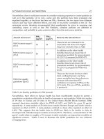
market applications. Tille [34] suggested an automotive air quality gas sensor using micro-
structured silicon technology as shown in Figure 10. The metallization and the gas-sensing
layer were electrically isolated from the heating layer by a passivation. Reducing gases (e.g.
CO, C
x
H
y
) result in an increase in conductivity and oxidizing gases (e.g. NO
2
) produce a
reduction in the conductivity of the metal oxide. For detection of various gases, several
sensor elements such as SnO
2
, ZnO, or WO
3
could be combined.

Fig. 10. Schematic illustration of a micro-structured metal oxide gas sensor (a) cross section;
(b) metallization as inter-digital structure, and heating layer as platinum meander structure;
(c) cross section of a typical automotive air quality sensor with embedded metal oxide gas
sensor [34].
In the future, smart sensors with high sensitivity, good reliability, and rapid response by
using MEMS technology and advanced signal processing should be developed.
4. References
[1] H. Kawasaki, T. Ueda, Y. Suda, and T. Ohshima, Sensors and Actuators B, vol. 100, p. 266,
2004.
[2] U. Guth and J. Zosel, Ionics, vol. 10, p. 366, 2004.
[3] K. S. Yoo, T. S. Kim, and H. J. Jung, J. Kor. Ceram. Soc., vol. 32, p. 1369, 1995.
[4] D. L. West, F. C. Montgomery, and T. R. Armstrong, Sensors and Actuators B, vol. 106, p.
758, 2005.
[5] Y. S. Yoon, T. S. Kim, and W. K. Choi, J. Kor. Ceram. Soc., vol. 41, p. 97, 2004.
[6] H. S. Kang, S. W. Kim, and Y. J. Cho, J. Kor. Furni. Soc., vol. 18, p. 91, 2007.
[7] J. H. Jang and Y. S. Lee, J. Archi. Ins. Kor., vol. 24, p. 299, 2004.
[8] H. J. An, C. H. Cheong, H. J. Kim, and Y. G. Lee, J. Archi. Ins. Kor., vol. 25, p. 51, 2005.
[9] J. Y. Park and M. S. Jung, J. Soc. Health Edu. Promo., vol. 1, p. 260, 1996.
[10] J. W. Seo, J. Kor. Air-Condi. Refri., vol.31, p. 13, 2002.
[11] Japanese R&D Trend Analysis Report No. 6: Ceramic Sensors, KRI International, Inc.,
Tokyo, 1989.
[12] J. S. Wilson, Sensor Technology Handbook, Elsevier, New York, 2005.
[13] S. Y. Yurish and M. T. S. R. Gomes, Smart Sensors and MEMS, Kluwer Academic
Publishers, Dordrecht, 2004.
[14] D. D. Lee, Ceramist, vol. 4, p. 57, 2001.

Monitoring, Control and Effects of Air Pollution

56
[15] T. S. Kim, Y. B. Kim, K. S. Yoo, K. S. Sung, and H. J. Jung, J. Kor. Ceram. Soc., vol. 34, p.
387, 1997.
[16] T. G. Nenov and S. P. Yordanov, Ceramic Sensors: Technology and Applications,
Technomic Publishing Company, Inc., Lancaster, 1996.
[17] ] M. W. Son, J. B. Choi, H. J. Kim, K. S. Yoo, and S. D. Kim, J. Kor. Phys. Soc., vol. 54, p.
1072, 2009.
[18] H. B. Shim, J. H. Kang, J. W. Choi, and K. S. Yoo, J. Electroceram., vol. 17, p. 971, 2006.
[19] M. W. Son, J. B. Choi, H. I. Hwang, and K. S. Yoo, J. Kor. Sensors Soc., vol. 18, p. 263,
2009.
[20] Wikipedia, 2011.
[21] "Reports", WorstPolluted.org., Retrieved 2010-08-29
by Wikipedia.
[22] "EPA: Air Pollutants", Retrieved
2010-08-29 by Wikipedia.
[23] Evidence Growing of Air Pollution’s Link to Heart Disease, Death // American Heart
Association, http//www.newsroom.heart.org/index.php?s=43&item=1029.
Retrieved 2010-05-10 by Wikipedia.
[24] "Newly Detected Air Pollutant Mimics Damaging Effects of Cigarette Smoke",
Retrieved 2010-08-29 by Wikipedia.
[25] "Infant Inhalation of Ultrafine Air Pollution Linked to Adult Lung Disease",
Retrieved
2010-08-29 by Wikipedia.
[26] A. H. Goldstein, D. K. Charles, L. H. Colette, and Y. F. Inez, Proc. National Academy of
Sci., 2009. Retrieved 2010-12-05
by Wikipedia.
[27] K. W. Jones, in: W. Göpel, J. Hesse, and J. N. Zemel (Ed.), Sensors, vol. 8, Micro- and
Nano Sensor Technology/ Trends in Sensor Markets, p. 451, VCH
Verlagsgesellschaft mbH, Weinheim, 1995.
[28] K. Colbow and K. L. Colbow, in: W. Göpel, J. Hesse, and J. N. Zemel (Ed.), Sensors, vol.

3, Chemical and Biochemical Sensors Part II, p. 969, VCH Verlagsgesellschaft mbH,
Weinheim, 1992.
[29] BITMART,
=&sc= &sn=, Seoul, Korea, 2009.
[30] G. Korotcenkov, Mater. Sci. & Eng. B, vol. 139, p. 1, 2007.
[31] F. Mitsugi, E. Hiraiwa, T. Ikegami, and K. Ebihara, Surface and Coatings Technology, vol.
169, p. 553, 2003.
[32] H. Kawasaki, J. Namba, K. Iwatsuji, Y. Suda, K. Wada, K. Ebihara, and T. Ohshima,
Applied Surface Sci., vol. 197, p. 547, 2002.
[33] C Y. lin, Y Y. Fang, C W. Lin, J. J. Tunney, and K C. Ho, Sensors and Actuators B, vol.
146, p. 28, 2010.
[34] T. Tille, Procedia Eng. (Proc. Eurosensors XXIV, Linz, Austria), vol. 5, p. 5, 2010.
[35] L. Bissi, M. Cicioni, P. Placidi, S. Zampolli, I. Elmi, and A. Scorzoni, IEEE Transactions on
Instrumentation and Measurement, vol. 60, p. 282, 2011.
[36] A. Serra, M. Re, M. Palmisano, M. V. Antisari, E. Filippo, A. Buccolieri, and D. Manno, ,
Sensors and Actuators B, vol. 145, p. 794, 2010.
[37] P G. Su and T T. Pan, Mater. Chem. and Phys., vol. 125, p. 351, 2011.

Gas Sensors for Monitoring Air Pollution

57
[38] U. Lange, V. M. Mirsky, Analytica Chimica Acta, vol. 687, p. 7, 2011.
[39] J. D. Fowler, M. J. Allen, V. C. Tung, Y. Yang, R. B. Kaner, and B. H. Weiller, ACS Nano,
vol. 3, p. 301, 2009.
[40] T. Kida, Y. Miyachi, K. Shimanoe, and N. Yamazoe, Sensors and Actuators B, vol. 80, p.
28, 2001.
[41] Y. Miyachi, G. Sakai, K. Shimanoe, and N. Yamazoe, Sensors and Actuators B, vol. 93, p.
250, 2003.
[42] H. J. Kim, H. B. Shim, J. W. Choi, and K. S. Yoo, Proc. 10th Asian Conf. on Solid State
Ionics, Kandy, Sri Lanka, p. 849, 2006.

[43] H. J. Kim, J. W. Choi, S. D. Kim, and K. S. Yoo, Mater. Sci. Forum, vols. 544-545, p. 925,
2007.
[44] J. J. Lai, H. F. Liang, Z. L. Peng, X. Yi, and X. F. Zhai, J. Phys.: Conf. Series (3
rd
Internaional
Photonics & OptoElectronics Meetings), vol. 276, p. 012129, 2011.
[45] F. Qiu, L. Sun, X. Li, M. Hirata, H. Suo, and B. Xu, Sensors and Actuators B, vol. 45, p. 233,
1997.
[46] J. P. Boilot, P. Salanié, G. Desplanches, and D. Le Potier, Mater. Res. Bull., vol. 14, p. 1469,
1979.
[47] D. H. H. Quon, T. A. Wheat, and W. Nesbitt, Mater. Res. Bull., vol. 15, p. 1533, 1980.
[48] G. Desplanches, M. Rigal, and A. Wicker, Am. Ceram. Soc. Bull., vol. 59, p. 546, 1980.
[49] N. Miura, S. Yao, Y. Shimizu, and N. Yamazoe, Sensors and Actuators B, vol. 9, p. 165,
1992.
[50] Y. Sadaoka, Y. Sakai, M. Matsumoto, and T. Manabe, J. Mater. Sci., vol. 28, p. 5783, 1993.
[51] S. Yao, Y. Shimizu, N. Miura, and N. Yamazoe, Chem. Lett., vol. 1990, p. 2033, 1990.
[52] N. Miura, S. Yao, Y. Shimizu, and N. Yamazoe, J. Electrochem. Soc., vol. 139, p. 1384,
1992.
[53] S. Yao, Y. Shimizu, N. Miura, and N. Yamazoe, Jpn. J. Appl. Phys., vol. 31, p. L197, 1992.
[54] Y. Shimizu, and N. Yamashita, Sensors and Actuators B, vol. 64, p. 102, 2000.
[55] T. Kida, H. Kawate, K. Shimanoe, N. Miura, and N. Yamazoe, Solid State Ionics, vol. 136,
p. 647, 2000.
[56] S. Zhao, J. K. O. Sin, B. Xu, M. Zhao, Z. Peng, and H. Cai., Sensors and Actuators B, vol.
64, p. 83, 2000.
[57] V. Lantto, S. Saukko, N. N. Toan, L. F. Reyes, and C. G. Granqvist, J. Electroceram., vol.
13, p. 721, 1992.
[58] I. Waernhus, N. Sakai, H. Yokokawa, T. Grande, M. Einarsrud, and K. Wiik, Solid State
Ionics, vol. 178, p. 907, 2007.
[59] M. Popa, J. Frantti, and M. Kakihana, Solid State Ionics, vols. 154 – 155, p. 437, 2002.
[60] H. K. Hong, B. H. Kim, Y. I. Cheon, and Y. K. Sung, J. Kor. Elect. Eng., vol. 13, p. 372,

1990.
[61] N. N. Toan, S. Saukko, and V. Lantoo, Physica B, vol. 327, p. 297, 2003.
[62] Z. Zhong, K. Chen, Y. Ji, and Q. Yan, Appl. Catalysis A : General , vol. 156, p. 29, 1997.
[63] S D. kim, B J. kim, J H. Yoon, and J S. Kim, J. Kor. Phys. Soc., vol. 51, p. 2069, 2007.
[64] B. Bahrami, A. Khodadadi, M. Kazemeini, and Y. Mortazavi, Sensors and Actuators B,
vol. 133, p. 352, 2008.
[65] M. W. Son, J. B. Choi, H. I. Hwang, and K. S. Yoo, J. Kor. Sensors Soc., vol. 18, p. 263,
2009.

Monitoring, Control and Effects of Air Pollution

58
[66] Z. A. Ansari, S. G. Ansari, T. Ko, and J H. Oh, , Sensors and Actuators B, vol. 87, p. 105,
2002.
[67] C T. Wang and M T. Chen, Sensors and Actuators B, vol. 150, p. 360, 2010.
[68] T. Fujioka, S. Kusanagi, N. Yamaga, Y. Watabe, K. Doi, T. Inoue, T. Hatai, K. Sato, A.
Takemoto, and D. Kouzeki, in: M. Aizawa (ed.), Chemical Sensor Technology, vol.
5, p. 65, Kodansha Ltd., Tokyo, 1994.
[69] Y. Shang, X. Wang, E. Xu, C. Tong, and J. Wu, Analytica Chimica Acta, vol. 685, p. 58,
2011.
[70] J Y. Leng, X J. Xu, N. Lv, H T. Fan, and T. Zhang, J. Colloid & Interface Sci., vol. 356, p.
54, 2011.
[71] N. V. Hieu, V. V. Quang, N. D. Hoa, and D. Kim, Current Appl. Phys., vol. 11, p. 657,
2011.
[72] P. Song, Q. Wang, and Z. Yang, Mater. Letters, vol. 65, p. 430, 2011.
[73] J. Gong, Q. Chen, M R. Lian, N C. Liu, R. G. Stevenson, and F. Adami, Sensors and
Actuators B, vol. 114, p. 32, 2006.
[74] T. V. Cuong, V. H. Pham, J. S. Chung, E. W. Shin, D. H. Yoo, S. H. Hahn, J. S. Huh, G. H.
Rue, E. J. Kim, S. H. Hur, and P. A. Kohl, Mater. Letters, vol. 64, p. 2479, 2010.
[75] G Y. Adachi and N. Imanaka, in: N. Yamazoe (ed.), Chemical Sensor Technology, vol.

3, p. 131, Kodansha Ltd., Tokyo, 1991.
[76] T. Takada, in: T. Seiyama (ed.), Chemical Sensor Technology, vol. 2, p. 59, Kodansha
Ltd., Tokyo, 1989.
[77] M. Blaschke, T. Tille, P. Robertson, S. Maier, U. Weimar, and H. Ulmer, IEEE Sensors J.,
vol. 6, p. 1298, 2006.


4
Development of Low-Cost Network of Sensors
for Extensive In-Situ and Continuous
Atmospheric CO2 Monitoring
Kuo-Ying Wang
1
, Hui-Chen Chien
2
and Jia-Lin Wang
3

1
Department of Atmospheric Sciences, National Central University,
2
Environmental Protection Administration,
3
Department of Chemistry, National Central University,
Taiwan
1. Introduction
Extensive and dedicated measurements of carbon dioxide concentrations in the atmosphere
are increasingly recognized as a necessary step in verifying anthropogenic carbon dioxide
emissions and as necessary methods to support international climate agreements (Marquis
& Tans, 2008; NRC, 2010; Tollefson, 2010). The successful launch of the Greenhouse Gas

Observing Satellite (GOSAT) on 23 Jan 2009 by Japan’s Aerospace Exploration Agency
(Heimann, 2009), followed by a not successful launch of Orbiting Carbon Observatory
(OCO) on 24 Feb 2009 (Brumfiel, 2009; Kintisch, 2009) all vindicate the importance of
extensive and accurate carbon dioxide measurements as a necessary step in global carbon
emission verification (Haag, 2007; Normile, 2009; Tollefson & Brumfiel, 2009). We note that a
replacement to the OCO is now actively in plan in NASA (Hand, 2009). Other satellite
instruments such as Aqua AIRS (Chahine et al., 2006), and SCIAMARCHY (Barkley et al.,
2006) have also provided retrieved CO2 concentration in the vertical column.
In Europe, an ongoing new research infrastructure called Integrated Carbon Observing
System (ICOS) is dedicated to establish and harmonize a network of atmospheric
greenhouse sites (). A list of present-day carbon dioxide
monitoring sites whose standard gases have traceability to the World Meteorological
Organization (WMO) standard is reported in WDCGG (2007).
In addition to these satellite remote sensing measurements and land-based in-situ
measurements, carbon dioxides also been measured from in-service commercial aircrafts
such as CONTRAIL (Matsueda & Inoue, 1996; Machida et al., 2008) and the planned flights
of IAGOS (Volz-Thomas et al., 2007), research aircraft such as the HIPPO
( and in-service container
cargo ships (Watson et al., 2009;).
Given the important status of carbon dioxide in affecting earth’s climate, however, detailed
measurements of carbon dioxide close to areas with heavy industrial emissions and intense
anthropogenic activities are relatively rare (Tollefson, 2010). This is in a sharp comparison
with other intensively observed air pollutants such as ozone, carbon monoxide, nitrogen

Monitoring, Control and Effects of Air Pollution

60
oxides, sulfur dioxide, and suspended particles. Since detailed measurements of carbon
dioxides close to anthropogenic areas where carbon dioxide is being relentlessly emitted
into the atmosphere are required to estimate its annual emission inventories (NRC, 2010),

more portable and flexible measurements but in the meantime accurate and traceable to
WMO standards are needed to significantly increase carbon dioxide measurements where
carbon dioxide been emitted. Burns et al. (2009) described a portable trace-gas measuring
system to measure carbon dioxide. In this work we develop a GFC-based measurement
system for extensive carbon dioxide measurements that are traceable to the WMO NOAA
CO2 standards.
2. Method
In this work we use a fast-response high-precision CO2 analyzer as the core for our CO2
measurements. The analyzer, EC9820T, was made by ECOTECH, Australia (ECOTECH,
2007). The EC9820T was built based on the principle of gas filter correlation (GFC) and the
nondispersive infrared (IR) absorption of CO2 near 4.5 microns which is used to determine
the presence of the CO2.


Fig. 1. A top view of the EC9820 CO2 analyzer.
Fig. 1 shows a photo of the top view of the CO2 analyzer used in this work. The analyzer
comprises three basic components: the sample flow components (valve manifold, particulate
filter, pump, Teflon tubes, dryer, etc), the optical measurement components (motor, IR
sources, measurement cell, IR detector), and computer control component (microprocessor
boards located at the lower half of the unit, power supply, and fan).
Development of Low-Cost Network of Sensors for
Extensive In-Situ and Continuous Atmospheric CO2 Monitoring

61

Fig. 2. A schematic diagram showing the major component of the EC9820 CO2 analyzer
(ECOTECH, 2007).
The exact locations of these components are shown in more details in Fig. 2. The FRONT
presents a mini-terminal like operational interface where the operations and calibrations of
the analyzer can be done from this region. The REAR indicates area where sample flow

tubes (including ZERO CO2 airs, span gases, exhaust, and purged air which provide zero
CO2 air to the chamber that houses gas correlation wheel) are connected with the analyzer.
The optical components are the locations where the GFC principle is in action and
measuring the atmospheric CO2 concentrations. The measured results are stored in the
onboard computer storages. The measurement cycles, and the control of manifold valves
where different airs (zero CO2 air, span CO2 airs, and sample air) are entirely controlled by
the onboard microprocessor unit. The analyzer analyzes CO2 concentrations, using the GFC
principle, and stores the analyzed (measured) results in the onboard computer storage area.
This distinctive capability makes the analyzer a self contained unit which is
characteristically suitable to conduct portable and accurate CO2 measurements that are
traceable to WMO NOAA standards. The independent of the analyzer from the need of an
additional data logger makes the entire operation understandable and sustainable.
Fig. 3 is a flow chart showing a typical loop for sample air measurement. The sample air is
sucked in from the SAMPLE IN (on the left) by the the PUMP which connected to SAMPLE
EXHAUST (on the right). The pump maintains the sample flow rates at 1 liter per minute. The
sample air first passes filter paper where filters our suspended particles in the sample before
entering the measurement cell. On the top, the MOTOR drives the rotation of gas filter wheel,
which is illuminated with the broadband IR sources (more details of the operational principle
of IR sources and gas filter wheel will be discussed later). The DETECTOR detects the
concentrations of CO2 in the sample air, and the electrical signals are sent to preprocessor and
micro processor boards to determine and store the measured results.

Monitoring, Control and Effects of Air Pollution

62

Fig. 3. A flow-chart diagram for the EC9820 CO2 analyzer (ECOTECH, 2007).


Fig. 4. A pneumatic diagram for EC9820 CO2 analyzer (ECOTECH, 2007).

Development of Low-Cost Network of Sensors for
Extensive In-Situ and Continuous Atmospheric CO2 Monitoring

63
Fig. 4 shows a pneumatic diagram of the CO2 analyzer. The externally given zero CO2 air,
span gases, and sample airs are input to the analyzer through the electronic valve manifold.
The span gases normally comprise of two working standards which are calibrated against
WMO NOAA CO2 standards provided by NOAA ESRL CCL. All inlet airs pass through a
particulate filter to remove suspended particle in the air. The inlet air then enters the
measurement cell where GFC principle used to measure CO2 levels. Additional zero CO2
air is provided through auxiliary (AUX) inlet at a flow rate of0.5 liter per minute. The
purpose of this purge air is to fill the chamber that houses gas correlation wheel and the IR
source with zero CO2 air therefore the interference of CO2 between IR source and gas
correlation wheel can be removed.


Fig. 5. A schematic diagrame showing the optical component of the analyzer (ECOTECH,
2007)
More detailed structure of GFC principle used in measuring CO2 levels is shown in Fig. 5.
From the left-most part is the motor, which rotates the gas filter correlation wheel. Between
the motor and the wheel is a broadband IR sources that constantly emit IR sources to the
two small chambers that enclose pure CO2 and N2 airs, respectively (Fig. 6). When the IR
sources pass CO2 chamber, the IR centered at 4.5 microns will be absorbed and removed
while the rest IR spectrums pass CO2 chamber and enter the measurement cell. On the other
hand, when the IR sources pass N2 chambers, nothing will be absorbed by the N2 chamber
and all IR sources enter the measurement cell where the absorption at 4.5 microns will be
occurred due to the CO2 in the measurement cell. The IR sources then pass a narrow band
pass filter that allow near 4.5 microns the leave the measurement cell and to be detected by
the IR detector on the right-most part.
GFC-based technology has been extensively used for providing CO measurements in the

atmosphere (Dickerson & Delany, 1988; Doddridge et al., 1994; Doddridge et al., 1998;
Gerbig et al., 1999; Novelli, 1999; Chen and Xu, 2004; Wong et al, 2007; Zellweger et al.,
2009).

Monitoring, Control and Effects of Air Pollution

64

Fig. 6. A schematic diagram showing the top and side views of the gas correlation wheel
used in the optical component of the analyzer (ECOTECH, 2007).
3. Results
3.1 Constant SPAN test


Fig. 8. A constant span test for a CO2 analyzer in the laboratory.
Development of Low-Cost Network of Sensors for
Extensive In-Situ and Continuous Atmospheric CO2 Monitoring

65
A total of eleven EC9820 CO2 analyzers have been installed since June 2009 for atmospheric
CO2 measuring. Each CO2 analyzer was tested in the laboratory before start taking
measurements. Fig. 8 shows a constant span test that run continuously for 48 hours using a
given working standard. This test was run with 2-hour background frequency (the white
gas seen in the data). The output frequency is 2 seconds. The results show that the
instrument is very stable from this continuous span test. The constant span tests, and later
added constant zero CO2 tests, are good ways to rigorously test if an analyzer is stable and
fit for making measurements.
3.2 Inter comparisons between analyzers

Fig. 9. Inter comparisons of CO2 sample measurements (raw data, in the units of ppm)
between three analyzers for the period from 28 October to 4 November 2009.


Fig. 10. Intercomparisons of CO2 sample measurements (raw data, in the units of ppm)
between two analyzers for the period from 28 October to 4 November 2009.

Monitoring, Control and Effects of Air Pollution

66
In addition to the constant span tests and zero tests, analyzers were continuously tested
against each other in the laboratory. Fig. 9 shows a time-series plot of a test run between
three CO2 analyzers from 28 October 4 November 2009. The results shown here are raw
data (un-calibrated data), which shows great consistency in these analyzers. Fig. 10 shows
another test results from inter comparisons of two analyzers in a second laboratory. The
occasional short bursts of high CO2 concentrations close to 500 ppm were resulted from the
researchers making routine maintenance and download of data from the analyzers. Fig. 10
very nicely show that measurements are consistent with each other; and the effect of human
presence can be quickly response in the measured data.
3.3 Inter comparisons between GFC and CRDS analyzers


Fig. 11. Inter comparisons of CO2 measurements between GFC and CRDS-based analyzers
for the period from 25 November to 8 December 2009
During the period of late 2009 and early 2010, we have had a chance to have an analyzer
based on cavity ring down spectroscopy (CRDS) principle running in our laboratory. This
analyzer was built by Los Gatos Research Inc., USA(van der Lann et al., 2009). Fig. 11 shows
a comparison of time-series plot for the period from 25 November to 8 December 2009.
These results indicate a good consistency between the measurements (correlation
coefficient= 0.99).

3.4 CO2 measurements in campus
Fig. 12 shows a time-series plot of CO2 measurements at two sites in the campus of National
Central University (NCU) for the period from 13 to 21 February 2010. These two sites are
separated by 400 m. One analyzer has its sample inlet located at 15 meter height (blue
Development of Low-Cost Network of Sensors for
Extensive In-Situ and Continuous Atmospheric CO2 Monitoring

67
curve), while the other analyzer has its sample inlet located at 35 meter height (red curve).
Both measurements were conducted with two working standards that are traceable to WMO
NOAA standards. Fig. 12 shows that the measurements are very consistent with each other.
The period from 24 to 19 February 2010 is the Chinese New Year in Taiwan, and the
measured CO2 concentrations are basically very close to 400 ppm and with little variations.
However, after the long holiday was over, the return of working people clearly impacted
CO2 levels as shown in the days on 20 and 21 February 2010. After 22 February 2010, Fig. 13
shows variations of CO2 during the normal human activity. The CO2 concentrations vary
between 400 and above 470 ppm. The sharp contrast between the long holiday period (Fig.
12) and normal working days (Fig. 13) clearly shows the impact of anthropogenic activity on
the atmospheric CO2 concentrations.


Fig. 12. A time-series plot shown CO2 measurements at two site in the campus of National
Central University (NCU) for the period from 13 to 21 February 2010.


Fig. 13. CO2 measurements at a site in the campus for the period from 22 February to 2
March 2010.

Monitoring, Control and Effects of Air Pollution

68

Fig. 14. Time-series plots of CO2 measurements (in the units of ppm) at two sites (blue curve
indicates results from 15-m height sample inlet, red curves indicates results from 35-m
height sample inlet) in the NCU campus for the period from 12 to 17 May 2010.
Fig. 14 shows another comparison of continuous CO2 measurements at two sites in the NCU
campus. Again, we observe the great consistency of CO2 measurements. These results
vindicate that our methodology can be consistently applied for a long period, and the use of
the GFC-based analyzer with the working standards traceable to WMO NOAA standards
ensure that our measurements meet WMO requirements (WDCGC, 2007).
3.5 Indoor CO2 measurements


Fig. 15. Indoor CO2 measurements taken in a classroom with 30 students inside on 8 Mar 2010.
Development of Low-Cost Network of Sensors for
Extensive In-Situ and Continuous Atmospheric CO2 Monitoring

69
In addition to outdoor CO2 measurements shown before, we have also conducted indoor
CO2 measurements to understand the variations of CO2 inside a room. Fig. 15 shows a time-
series plot of CO2 measurements in a classroom with 30 students at NCU campus on 8 Mar
2010. The build up of the CO2 from 14:30 to 15:20 local time was due to the close of both
doors of the classroom. The reduction from about 15:20 to 17:00 was due to the open of a
door for ventilation (the air was too stuffy). The effect of ventilation in removing indoor
accumulation of CO2 is clearly seen in these results. The measurements also nicely contrast
indoor CO2 concentrations with those coming for ambient air, which was taken after 17:00
local time.


Fig. 16. Indoor CO2 measurements taken in a 100-people working office for the period from

9 Mar to 16 Mar 2010.
Fig. 16 shows another indoor CO2 measurement taken in a 100-people working office for the
period from 9 to 16 Mar 2010. Here we see clearly the daily accumulation of CO2 inside the
office from about 08:00 local time to peak at about 13:00-15:00 in the early afternoon. The
reductions after 15:00 are due to the gradual leaving of people from the office and the
accumulated effect of ventilation to counter the CO2 accumulation inside the office. The
smooth CO2 concentrations inside the office during the weekend (13-14 March) are clearly
seen.
3.6 CO2 measurements onboard a in-service container ship
One of the main motivations to develop GFC-based CO2 measurements is to conduct global
CO2 measurements over the Pacific regions. We have vigorously tested this idea since June
2009. Fig. 17 shows a service route from a container ship called EVER DECENT during its
service for the period from 22 January to 26 Mar 2010. The detailed operations and
installation of the GFC analyzer and CO2 working standards will be reported in a separate
work. Fig. 18 shows results from this cruise. The measurements show that CO2 levels are
close to 400 ppm when the measurements were taken over the marine atmospheric
boundary layer. However, the CO2 levels increase sharply as soon as the ship approached a
port. This plot very nicely shows that anthropogenic activity as the key sources for
atmospheric CO2 levels. More results on the ship-based measurements will be presented in
separate publications this year.

Monitoring, Control and Effects of Air Pollution

70

Fig. 17. A service route for EVER DECENT for the period from 22 Janunary to 26 Mar 2010.


Fig. 18. A time-series plot of a ship-based measurement made by EVER DECENT
4. Summary

In this work we demonstrate the development of a GFC-based technology for making
continuous in-situ atmospheric CO2 measurements for climate policy decision makers. All
GFC-based analyzers were rigorously tested in the laboratory before went to the field for
measurements. All CO2 measurements were made with two CO2 working standards that
are traceable to the WMO NOAA CO2 standards. All CO2 working standards were
routinely calibrated again six bottles of WMO NOAA CO2 standards.
Great effort has been taken to ensure that the atmospheric CO2 measurements follow the
WMO standards (WDCGC, 2007). We have developed a series of tests to verify the
measurements, including constant span test, constant zero tests, inter comparisons between
GFC analyzers, and inter comparisons between GFC and a CRDS analyzer. We show some
results from the land-based measurements taken in the NCU campus, indoor
measurements, and a ship-based measurement. These results indicate encouraging results
that can significantly increase our understanding of atmospheric CO2 distribution.
5. Acknowledgements
We are very grateful to National Science Council, and Environmental Protection
Administration, Taiwan, for funding this work. We benefit tremendously from the help,
comments, and continuous discussions from Neil Harris and Andrew Robinson of