Supply Chain Management Pathways for Research and Practice Part 6 doc

Bullwhip-effect and Flexibility in Supply
Chain Management 5
In consequence, the MAC inequality may be written in terms of the adjustment degree of
production as follows:
1
 ϑ
1
+ γ
1
− 1  ϑ
2
+ γ
2
− 1   ϑ
n
+ γ
n
− 1. (12)
This is an interesting result because, since Amp
i
measures the bullwhip-effect of a given
management system, when faced to a specific demand behavior, it suggests that monitoring of
ϑ
i
yields a more adequate feedback to the supply chain manager. In fact, it furnishes her/him
with a control variable in the supply chain. In the next section, this idea is explored for the
three ordering methods.
3.2 Flexibility conditions for an AR(1) demand process
A simple observation of Table 1 exposes the way that the adjustment behavior propagates
upstream in the supply chain. Inspecting the expression (12), a manager could rapidly
establish a control condition, when implementing a particular method. For instance, it is easy

to see that a hybrid method satisfies
2
 ϑ
1
+ γ
1
 ϑ
1
+ γ
2
  ϑ
1
+ γ
n
, (13)
whilst in a pull method with ϑ
i
= 0 (∀i), we have
2
 γ
1
 γ
2
  γ
n
. (14)
However, for a push method this condition needs to be found for every specific demand
process. Therefore, for sake of analysis, let us assume that the demand rate can be accurately
modeled by an i.i.d stationary AR(1) stochastic process with mean μ, variance σ
2

and
autocorrelation coefficient λ
∈ (−1, 1).
When a pull ordering method is adopted, using (1) and (4), we have P
i
t
= D
t−iL
. Hence, for a
stationary stochastic demand process it follows,
γ
i
=
2
V[D
t
]

E

(
D
t−iL
)
2

−
(
E
[

D
t−iL
])
2

= 2. (15)
Thus, the relation between ϑ
i
and Amp
i
is
Amp
i
= ϑ
i
+ 1. (16)
But ϑ
i
= 0, ∀i (see Table 1), which implies Amp
i
= 1. In consequence, a pull inventory
management simultaneously minimizes ϑ
i
and accomplishes the MAC criteria. Differently,
when a push ordering method is considered, using (1) and (2), we have
P
i
t
= D
t−iL

+
i
∑
j=1
Δ
ˆ
D
j
(
i+1−j
)
L
= D
t−iL
+ θ
i
t
. (17)
89
Bullwhip-Effect and Flexibility in Supply Chain Management
6 Will-be-set-by-IN-TECH
Therefore,
γ
i
=
2
V
[
D
t

]
{
V
[
D
t
]
+
E
⎡
⎣
D
t−iL
⎛
⎝
i
∑
j=1
Δ
ˆ
D
j
t
−
(
i+1−j
)
L
⎞
⎠

⎤
⎦
−E
[
D
t
]
E
⎡
⎣
i
∑
j=1
Δ
ˆ
D
j
t
−
(
i+1−j
)
L
⎤
⎦
⎫
⎬
⎭
, (18)
This equation shows that in the push method, the relation between ϑ

i
and Amp
i
depends
on the first and second order statistics of the demand stochastic process able to describe
the requested units. A closed expression can be found for some specific demand stochastic
processes. In particular, given an AR(1) stochastic demand process, a straightforward analysis
shows that

ˆ
D
i
t
=(D
t
− D
t−1
)
L+1
∑
j=1
λ
LT
(i−1)
+j
=(D
t
− D
t−1
)λ

LT
(i−1)
φ. (19)
where φ
= λ
λ
L+1
−1
λ−1
, λ = 1. Knowing that E

D
t−k
D
t−j

= λ
k−j
σ
2
+ μ
2
, ∀k > j, we find an
expression for γ
i
, expressed as
γ
i
= 2 + 2
(

λ − 1
)
φ
i
∑
j=1
λ
LT
(j−1)
−
(
1−j
)
L−1
= 2 + 2

λ
L+1
− 1

1
− λ
2Li
1 − λ
2L
. (20)
From this equation, γ
i
− γ
i−1

≤ 0. In addition, (11) and Table 1 imply ϑ
i
= Am p
i−1
− γ
i−1
− 1
and ϑ
i
= ϑ
i−1
+ H
i
, respectively. Then
Amp
i
= Am p
i−1
+ γ
i
− γ
i−1
+ H
i
. (21)
Now, let us restrict ϑ
i
such that
ϑ
1

 ϑ
2
  ϑ
n
, (22)
meaning that H
i
≤ 0, ∀i. In such case, (21) implies Amp
i−1
≥ Amp
i
, ∀i, and the MAC
condition would be satisfied. Unfortunately, in a previous publication we have shown that
H
i
≤ 0 is rarely satisfied and for most of λ values we have ϑ
i
≥ ϑ
i−1
(Pereira and Paulre,
2001). For this reason, a different strategy needs to be explored. Actually, given that the MAC
condition is immediately satisfied by a pull method, it could be interesting to know how
amplification is reduced when a push or hybrid method moves closer to the pull case. In the
next section such idea is analyzed, introducing a fading variable which models the manager’s
belief on demand forecasting.
90
Supply Chain Management – Pathways for Research and Practice
Bullwhip-effect and Flexibility in Supply
Chain Management 7
3.3 The manager’s belief effect

In Pereira et al. (2009) we proposed an alternative to control the bullwhip-effect, using a
learning variable representing the manager’s belief on the forecasted demand change. This
learning was modeled by a factor α, included in the ordering equation as O
i
t
= P
i−1
t
+ α
ˆ
D
i
t
,
which conveys θ
i
t
= α
ˆ
D
i
t
. Applying the same procedure yielding the results on Table 1
(Pereira and Paulre, 2001), it is straightforward to prove that the amplification value on stage
i, Amp
i
α
, is expressed as follows,
Amp
i

α
=

1
+ A
α
i = 1,
Amp
i−1
α
+ F
i
α
i > 1.
(23)
In particular, when the AR(1) process is considered, we find
A
α
= 2αφ(1 − λ)(αφ + 1), (24)
F
i
α
= 2αφ(1 − λ)λ
2(i−1)L
{αφ −
1
λ
− φ
1
− λ

λ
(i − 1)} (i = 2, ,n). (25)
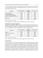
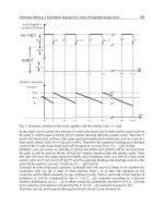
In Fig. 2 amplification for α
∈ [0, 1], L = 1, λ ∈ (−1, 1) and i ∈{2, 8} is presented. Notice
that for i
= 2 and the region λ ≥ 0, the more α increases the more the bullwhip-effect is
important, but the greatest amplification value is not reached as λ approaches 1. On the other
hand, results for i
= 8 (Fig. 2(b)) are not intuitive and suggest that the improvement strategy
consisting on the progressive reduction of the adjustment degree, by decreasing α, does not
necessarily reduce the bullwhip-effect. Even though, one may conclude that in push or hybrid
methods, the bullwhip-effect is robustly reduced when stages approaches a pull-type ordering
method. In other words, a manager is not necessarily enforced to abandon the push strategy
to obtain acceptable amplification levels, but she/he should make a careful analysis in order
to appreciate the consequences of his beliefs about the demand behavior and estimates.
Now, it is interesting to know how the inventory amplification level is shaped by the demand
process. In particular, the way that the belief variable influences such level. Therefore, let us
define Iamp
(i−1)
(i = 1, . . . , n) as the inventory amplification of the stock site B
i−1
, that is
Iamp
(i−1)
=
V(B
(i−1)
t
)
V(D

t
)
. (26)
It has been demonstrated that the production amplification impacts the inventory fluctuation,
in the way depicted in Table 2 (Pereira, 1995). In general, ψ
i
and ν
i
(i = 1, . . . , n) are complex
expressions depending on the forecasted and real demand processes. Instead, let us consider
the expression (27), which represents the amplification level of the marginal inventory change,
Amp
B
i−1
=
V(B
(i−1)
t
− B
(i−1)
t−1
)
V(D
t
)
. (27)
Stage Push Hybrid Pull
i = 1 Amp
1
+ ψ

1
Amp
1
+ ψ
1
Amp
1
+ ν
1
i > 1 Amp
i
+ ψ
i
Amp
i
+ ν
i
Amp
i
+ ν
i
Table 2. Amplification of inventory InvAmp
(i−1)
for the three management methods
91
Bullwhip-Effect and Flexibility in Supply Chain Management
8 Will-be-set-by-IN-TECH















Amp
i
(a) i = 2



















Amp
i
(b) i = 8
Fig. 2. Amplification when α ∈ [0, 1], L = 1 and i = 2, 8 (Pereira et al. , 2009).
This variable measures how sensitive the inventory is to the demand process. Intuitively, the
more sensitive it is, the less smooth the inventory signal, when faced to the demand process.
Restricting ourselves to the case i
= 1 and given that B
0
t
= B
0
t
−1
+ P
1
t
−1
− D
t
, a straightforward
analysis reveals that, when the learning variable α is included in the model, the following
expression is obtained
Amp
B
0
α
= Am p

1
α
+ 1 − 2

λ
L+1
+ αφ(λ
L+1
− λ
L+2
)

(28)
= 2

1 + αφ

(1 − λ)(αφ + 1) − λ
L+1
+ λ
L+2

− λ
L+1

.
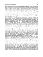
Figure 3 shows Amp
B
0
α

for α ∈ [0, 1] and λ ∈ (−1, 1), when L = 1. This indicates that the
inventory on stock site B
0
is actually sensitive to the belief variable meaning that a smoothing
effect should be expected if α is decreased for a given λ value. As qualitatively observed,
effectiveness of α is low for negative values of autocorrelation. Notice that the same kind
of phenomenon is observed in Figure 2: the more α decreases, the less the amplification
improves.
We may conclude that a fading action, implemented via the manager’s belief variable, may be
a sound strategy for reduction of the bullwhip effect, both on the production and inventory
sides, but only for specific values of autocorrelation. In particular, this kind of management
should be surely applied for low positive values of λ.
4. Conclusions
In a previous paper we proposed that flexibility aids in reduction of the bullwhip-effect in a
multi-echelon, single-item, supply chain model. In this chapter we have found a flexibility
condition that guarantees the control of the bullwhip-effect in the supply chain (expression
92
Supply Chain Management – Pathways for Research and Practice
Bullwhip-effect and Flexibility in Supply
Chain Management 9
−1
−0.5
0
0.5
1
0
0.2
0.4
0.6
0.8

1
0
0.5
1
1.5
2
2.5
3
λ
α
Amp
α
ΔB
0
Fig. 3. Marginal inventory change amplification on stock site B
0
, when α ∈ [0, 1].
(22)). This is an interesting result because it asks the manager for an ordering strategy that
synchronizes the flexibility among stages in the chain. However, such condition being difficult
to fulfill when an AR(1) demand process is considered, a different strategy has been explored.
Control of a learning variable, representing the manager’s belief on demand forecasting, has
been proposed here as an alternative strategy to regulate the bullwhip-effect. We have seen
that, although this strategy does not necessarily assure fulfillment of the MAC condition, it
may be an effective way to smooth production and inventory fluctuation. Our results indicate
that, under the model assumptions, the pull ordering method is highly robust, in the sense of
reduction of the amplification effect. Thus, the fading strategy suggested invites the supply
chain manager to improve synchronization among stages in the supply chain, becoming closer
to the pull method. Nevertheless, a manager is not necessarily enforced to abandon the push
strategy in order to obtain acceptable amplification levels, but she/he should make a careful
analysis assessing the consequences of his beliefs about the demand and estimates behavior.

Results presented in this chapter open to new ideas about the way that different fading
strategies impact the bullwhip-effect behavior. Even if an early study was proposed by Pereira
et al. (2009), the focus was rather mathematical and no framework was suggested as a specific
analytical grid. In consequence, future research concerns the hypothesis that decision makers
evidence limited rationality bias when facing an ordering method. Although this idea has
been already analyzed (Oliva and Gonçalves , 2005), we think that the availability heuristic
proposed by Tversky and Kahneman (1974), in our case concerning the overreaction to the
downstream information, could be successfully explored using our supply chain model.
5. Acknowledgment
This publication has been fully supported by the Universidad Diego Portales Grant VRA
132/2010.
93
Bullwhip-Effect and Flexibility in Supply Chain Management
10 Will-be-set-by-IN-TECH
6. References
Chen, F., Drezner, Z., Ryan, J., Simchi-Levi, D., 2000. Quantifying the bullwhip effect in
a simple supply chain: The impact of forecasting, lead times, and information.
Management Science 46 (3), 436–443.
Forrester, J., 1969. Industrial dynamics. The MIT Press, Cambridge, MA, USA.
Geary, D., Disney, S., D.R.Towill, 2006. On bullwhip in supply chains - historical review,
present practice and expected future impact. International Journal of Production
Research 101 (1), 2–18.
Lee, H., Padmanabhan, P., Whang, S., 1997. Information distortion in a supply chain: the
bullwhip-effect. Management Science 43 (4), 546–558.
Lee, H., So, K., C.Tang, 2000. The value of information sharing in a two-level supply chain.
Management Science 46 (5), 626–643.
Muramatsu, R., K.Ishi, Takahashi, K., 1985. Some ways to increase flexibility in manufacturing
systems. International Journal of Production Research 23 (4), 691–703.
Oliva, R., Gonçalves,P., 2005, Behavioral Causes of Demand Amplification in Supply Chains:
“Satisficing” Policies with Limited Information Cues. Proceedings of International

System Dynamics Conference, July 17 - 21, 2005, Boston.
Pereira, J., October 1995. Flexibilité dans les systèmes de production: analyse et évaluation par
simulation. Ph.D. thesis, Université Paris-IX Dauphine, France.
Pereira, J., July 1999. Flexibility in manufacturing processes: a relational, dynamic
and multidimensional approach. In: Cavana, R., Vennix, J., Rouwette, E.,
Stevenson-Wright, M., Candlish, J. (Eds.), 17th International Conference of the
System Dynamics Society and the 5th Australian and New Zealand Systems
Conference, Wellington, New Zealand. System Dynamics Society, pp. 63–75.
Pereira, J., Paulre, B., 2001. Flexibility in manufacturing systems: a relational and a dynamic
approach. European Journal of Operational Research 130 (1), 70–85.
Pereira, J., Takahashi, K., Ahumada, L., Paredes, F., 2009. Flexibility dimensions to control
bullwhip-effect in a supply chain. International Journal of Production Research, 47:
22, 6357–6374.
Sterman, J., 2006. Operational and behavioral causes of supply chain instability. In: Carranza,
O., Villegas, F. (Eds.), The Bullwhip Effect in Supply Chains. Palgrave McMillan.
Takahashi, K., Hiraki, S., Soshiroda, M., 1994. Flexibility of production ordering systems.
International Journal of Production Research 32 (7), 1739–1752.
Takahashi, K., Myreshka, 2004. The bullwhip effect and its suppression in supply chain
management. In: H. Dyckhoff, R. L., Reese, J. (Eds.), Supply Chain Management
and Reverse Logistics. Springer, pp. 245–266.
Tversky, A., Kahneman, D., 1974. Judgment Under Uncertainty: Heuristics and Biases. Science
185 (4157), 1124-1131.
Warburton, R., 2004. An analytical investigation of the bullwhip effect. Production and
Operations Management 13 (2), 150–160.
Wu, S., Meixell, M., 1998. Relating demand behavior and production policies in the
manufacturing supply chain. Tech. Rep. 98T-007, IMSE , Lehigh University.
94
Supply Chain Management – Pathways for Research and Practice
8
A Fuzzy Goal Programming Approach for

Collaborative Supply Chain Master Planning
Manuel Díaz-Madroñero and David Peidro
Research Centre on Production Management and Engineering (CIGIP)
Universitat Politècnica de València
Spain
1. Introduction
Supply chain management (SCM) can be defined as the systemic, strategic coordination of
the traditional business functions and the tactics across these business functions within a
particular company and across businesses within the supply chain (SC), for the purposes of
improving the long term performance of the individual companies and the SC as a whole
(Mentzer et al. 2001). One important way to achieve coordination in an inter-organizational
SC is the alignment of the future activities of SC members, hence the coordination of plans.
It is often proposed that operations planning in supply chains can be organized in terms of a
hierarchical planning system (Dudek & Stadtler 2005). This approach assumes a single
decision maker with total visibility of system details who makes centralized decisions for
the entire SC. However, if partners are reluctant to reveal all of their information or it is too
costly to keep the information of the entire supply chain up-to-date, the hierarchical
planning approach is unsuitable or infeasible (Stadtler 2005). Hence, the question arises of
how to link, coordinate and optimize production planning of independent partners in the
SC without intruding their decision authorities and private information (Nie et al. 2006).
Stadtler (2009) defines collaborative planning (CP) as a joint decision making process for
aligning plans of individual SC members with the aim of achieving coordination in light of
information asymmetry. Then, to generate a good production-distribution plan in a SC, it is
necessary to resolve conflicts between several decentralised functional units, because each
unit tries to locally optimise its own objectives, rather than the overall SC objectives. Because
of this, in the last few years, the visions that cover a CP process such as a distributed
decision-making process are getting more important (Hernández et al. 2009).
Selim et al. (2008) assert that fuzzy goal programming (FGP) approaches can effectively be
used in handling the collaborative production and distribution planning problems in both
centralized and decentralized SC structures. The reasons of using FGP approaches in this

type of problems are explained by Selim et al. (2008) as follows:
1. Collaborative planning is the more preferred mode of operation by today’s companies
operated in SCs. These companies may consent to sacrifice the aspiration levels for their
goals to some extent in the short run to provide the loyalty of their partners or to
strengthen their partners’ competitive position in the long term. In this way, they can
facilitate providing a long-term collaboration with their partners and subsequently
gaining a sustainable competitive advantage.

Supply Chain Management – Pathways for Research and Practice
96
2. Due to the impreciseness of the decision makers’ aspiration levels associated with each
goal, conventional deterministic goal programming (GP) approach cannot fully reflect
such complexity.
3. Collaborative planning problems in SCs are complex and mostly multiple objective
problems, and often include incommensurable goals. Incommensurability problem in
goal programming occurs when deviational variables measured in different units are
summed up directly. In goal programming technique, a normalization constant is
needed to overcome this difficulty. However, in FGP, incommensurable goals can be
treated in a reasonable and practical way.
Therefore, it may be appropriate to use FGP approaches in production and distribution
planning problems existing in real-world supply chains.
We arrange the rest of this work as follows. Section 2 presents a literature review about
integrated production and distribution planning models, as well as collaborative. Section 3
describes the FGP approaches to deal with supply chain planning problem in centralized
and decentralized SC structures. Section 4 presents a multi-objective, multi-product and
multi-period model for the master planning problem in a ceramic tile SC. Then, in Section 5,
the solution methodology and the FGP approaches for different SC structures (i.e.
centralized and decentralized) are described. Section 6 validates and evaluates our proposal
by using an example based on a real-world problem. Finally, Section 7 provides conclusions
and directions for further research.

2. Literature review
The considered ceramic supply chain master planning (CSCMP) problem deals with a
medium term production and distribution planning problem in a four-echelon ceramic tile
supply chain involving one manufacturer, multiple warehouses, multiple logistic centres
and multiple shops. The integration of production and distribution planning decisions is
crucial to ensure the overall performance of the SC, and has attracted attention both from
practitioners and academics for many years (Vidal & Goetschalckx 1997; Erengüç et al. 1999;
Bilgen & I. Ozkarahan 2004; Mula et al. 2010). According to Liang & Cheng (2009), in
production and distribution planning problems, the decision maker (DM) attempts to: (1) set
overall production levels for each product category for each source (manufacturer) to meet
fluctuating or uncertain demand for various destinations (distributors) over the
intermediate planning horizon and (2) make suitable strategies regarding regular and
overtime production, subcontracting, inventory, and distribution levels, and thus
determining appropriate resources to be used.
On supply chain planning, most prior studies have concentrated on formulating a
sophisticated supply chain planning model and devising an efficient algorithm to solve it
under a centralized supply chain environment where all supply chain participants are
grouped as one organization or company and all functions of a supply chain are fully
integrated by an independent planning department or supervisor (Jung et al. 2008).
According to Mula et al. (2010), the vast majority of works that deal with the production and
distribution integration opt for the linear-programming based approach, particulary mixed
integer linear programming models. Chen & Wang (1997) proposed a linear programming
model to solve integrated supply, production and distribution planning in a supply chain of
the steel sector. McDonald & Karimi (1997) presented a mixed deterministic integer linear
programming model to solve a production and transport planning problem in the chemical

A Fuzzy Goal Programming Approach for Collaborative Supply Chain Master Planning
97
industry in a multi-plant, multi-product and multi-period environment. Timpe & Kallrath
(2000) and Kallrath (2002) presented a couple of models for production, distribution and

sales planning with different time scales for business and production aspects. Dhaenens-
Flipo & Finke (2001) modelled a multi-facility, multi-item, multi-period production and
distribution model in the form of a network flow. Park (2005) suggested an integrated
transport and production planning model in a multi-site, multi-retailer, multi-product and
multi-period environment. Likewise, the author also presented a production planning
submodel whose outputs act as the input in another submodel with a transport planning
purpose and an overall objective of maximizing overall profits with the same technique.
Ekş{}ioğ{}lu et al. (2006) showed an integrated transport and production planning model in
a multi-period, multi-site, monoproduct environment as a flow or graph network to which
the authors added a mixed integer linear programming formulation. Later, Ekşioğlu et al.
(2007) extended this model to become a multi-product model solved by Lagrangian
decomposition. Ouhimmou et al. (2008) developed a mixed integer linear programming
(MIP) model for tactical planning in a furniture supply chain related to production and
logistics decisions. Fahimnia et al. (2009) proposed a model for the optimization of the
complex two-echelon supply networks based on the integration of aggregate production
plan and distribution plan.
According to Dudek & Stadtler (2005) the relevant literature on linking and coordinating the
planning process in a decentralized manner, distinguishes three main approaches:
coordination by contracts, multi-agent systems and mathematical programming models.
The largest number of references reviewed in Stadtler (2009) employs mathematical
decomposition (exact mathematical decomposition, heuristic mathematic decomposition
and meta-heuristics). Originally developed for solving large-scale linear programming,
mathematical decomposition methods seem to be an attractive alternative for solving
distributed decision-making problems. Barbarosoglu & Özgür (1999) developed a model
which is solved by Lagrangian and heuristic relaxation techniques to become a
decentralized two-stage model: one for production planning and another for transport
planning. It generates a final plan level by level, where one stage determines both its own
plan and supply requirements and passes the requirements to the next stage. Luh et al.
(2003) presented a framework combining mathematical optimization and the contract
communication protocol for make-to-order supply network coordination based in this

relaxation method. Nie et al. (2006) developed a collaborative planning framework
combining the Lagrangian relaxation method and genetic algorithms to coordinate and
optimize the production planning of the independent partners linked by material flows in
multiple tier supply chains. Moreover, Walther et al. (2008) applied a relaxation approach
for distributed planning in a product recovery network.
However, these examples require the presence of a central coordinator with a complete
control over the entire supply chain, otherwise there is no guarantee for convergence of the
final solution without extra modification procedure or acceptance functions because of the
duality gap or the oscillation of mathematical decomposition methods (Jung et al. 2008). In
this context, FGP can be a valid alternative to the previous drawbacks.
Fuzzy mathematical programming, especially the fuzzy goal programming (FGP) method,
has widely been applied for solving various multi-objective supply chain planning
problems. Among them, Kumar et al. (2004) and Lee et al. (2009) presented FGP approaches
for supplier selection problems with multiple objectives. Liang (2006) presented a FGP
approach for solving integrated production and distribution planning problems with fuzzy

Supply Chain Management – Pathways for Research and Practice
98
multiple goals in uncertain environments. The proposed model aims to simultaneously
minimize the total distribution and production costs, the total number of rejected items, and
the total delivery time. Torabi & Hassini (2009) proposed a multi-objective, multi-site
production planning FGP model integrating procurement and distribution plans in a multi-
echelon automotive supply chain network.
3. Modelling approaches for centralized and decentralized planning in SC
structures
3.1 Planning in centralized supply chain structure
According to their basic structures, SCs can be categorized as centralized and decentralized.
A supply chain is called centralized if a single dominant firm has all the information and
tries to, in the short run, simply optimize its own operational decisions regardless of the
impact of such decisions on the other stages of the chain (Erengüç et al. 1999). According to

Selim et al. (2008), FGP approaches can be used in handling collaborative master planning
problems in both centralized and decentralized SC structures. In order to handle the
problem in centralized SC, Selim et al. (2008) propose to use Tiwari et al. (1987) weighted
additive approach defined as follows:




0,1
0
kk
k
k
M
aximize w x
subject to k
x





(1)
In this approach, w
k
and
k

denotes the weight and the satisfaction degree of the kth goal
respectively. Therefore, the weighted additive approach allows the dominant partner in the

SC to assign different weights to the individual goals in the simple additive fuzzy
achievement function to reflect their relative importance levels.
3.2 Planning in decentralized supply chain structure
A SC is called decentralized when various decisions are made in different companies that
try to optimize their own objectives. Selim et al. (2008) state that the methods that take
account of min operator are suitable in modelling the collaborative planning problems in
decentralized SC structures. Among these methods, Selim et al. (2008) propose to use
Werners (1988) fuzzy and operator to address the SC collaborative planning problems in
decentralized SC structures. By adopting min operator into Werners’ approach the
following linear programming problem can be obtained:







11
,
,, 0,1
k
k
kk
k
Maximize K
sub
j
ect to x k K x X
  


 

  


(2)
where K is the total number of objectives, µ
k
is the membership function of goal k, and γ is
the coefficient of compensation defined within the interval [0,1]. In this approach, the
coefficient of compensation can be treated as the degree of willingness of the SC partners to
sacrifice the aspiration levels for their goals to some extent in the short run to provide the
loyalty of their partners and/or to strengthen their competitive position in the long run.

A Fuzzy Goal Programming Approach for Collaborative Supply Chain Master Planning
99
To explore the viability of the proposed fuzzy modelling approaches for the collaborative
SC planning in centralized and decentralized SC structures, we consider a supply chain
master planning problem related to a ceramic tile supply chain in the next section.
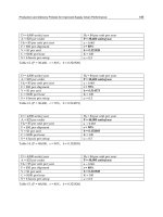
4. Model formulation
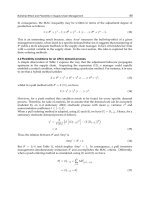
We adopt the ceramic supply chain master planning problem presented in Alemany et al.
(2010). Figure 1 shows the structure of a typical SC of the ceramic sector. The authors
describe the peculiarities related to these SCs and consider several assumptions. First, the
flow of parts, components, raw materials (RMs) and finished goods (FGs) that might
circulate between the nodes is known beforehand. The existence of several production
plants situated in various geographical locations is also assumed. These production plants
are supplied with various RMs provided by different suppliers with a limited supply
capacity.

Fig. 1. Ceramic tile SC considered in Alemany et al. (2010)
In the SC under study, each production plant has one or several parallel production lines,
which process different FGs, with a limited capacity. Moreover, there are FGs with high
added values that are manufactured only in production plants; others may be partly
subcontracted, while some may be totally subcontracted to external suppliers. FGs are
grouped into product families to minimize setup times and costs. A product family is
defined as a group of FGs with identical physical characteristics and whose preparation on
product lines is similar. Given the important setup times between product families on
production lines, minimum run lengths for product families are specified. Item setups
among the products belonging to the same product family also exist. Because of
technological factors involved in the production process itself, each product should be
produced in an equal or greater amount than the minimum lot size defined, when it’s
manufactured on a specific line.
Raw materials, item,
component suppliers
Production
plants
Central
warehouses
Logistic
centres
Shops
End
customers
Finished goods suppliers
Production lines
. . .
. . .
. . .
. . . . . . . . . . . .

Supply Chain Management – Pathways for Research and Practice
100
The distribution of FGs from production plants to end customers is carried out in various
stages by different types of distribution centres, such as central warehouses, logistic centres
and shops. Neither manufactured nor subcontracted FGs can be stored in manufacturing
plants. They are sent to the first distribution level which is composed of several central
warehouses with a limited storage capacity. The demand of end customers and logistics
centres is covered by the outgoing FGs from central warehouses. Besides, logistics centres
only supply FGs to shops that have been previously assigned to them. Finally, shops only
attend end costumers’ demand. Although a maximum service level is pursued in this SC,
limited backorders are permitted in both central warehouses and shops.
4.1 Nomenclature
The nomenclature defines the indices, sets of indices, parameters and decision variables
(Table 1).



Indices
c
RMs, items, and components
(c=1…C)
q
Logistic centres (q=1…Q)
i
FGs (i=1…I)
w
Shops (w=1…W)
f
Product families (f=1…F)

r
Suppliers of RMs, items, and
components (r=1…R)
l
Production lines (l=1…L)

p
Production plants (p=1…P)
b
Suppliers of finished products
(b=1…B)
a
Warehouses (a=1…A)
t
Periods of time (t=1…T)
Sets of Indices
Il(l)
Set of FGs that can be
manufactured on manufacturing
line l
Lp(p)
Set of manufacturing lines that
belong to production plant p
Fl(l)
Set of product families that can be
manufactured on manufacturing
line l
Pa(a)
Set of production plants that can
send FGs to warehouse a

If(f)
Set of FGs that belong to product
family f
Aq(q)
Set of warehouses that can supply
logistics centre q
Ip(p)
Set of FGs that can be produced in
production plant p
Rc(c)
Set of suppliers that can supply
RM c
Ia(a)
Set of FGs that can be stored in
warehouse a
Rp(p)
Set of suppliers of RMs that can
supply production plant p
Ic(c)
Set of FGs of that RM c form part
Cr(r)
Set of RMs that can be supplied
by supplier r
PFN
S
Set of FGs that cannot be
subcontracted
Qa(a)
Set of logistics centres that can be
supplied by warehouse a

PFSP
Set of FGs that can be
subcontracted either partially or
completely
Wq(q)
Set of shops that can be supplied
by logistics centres q

A Fuzzy Goal Programming Approach for Collaborative Supply Chain Master Planning
101
PFST
Set of FGs that are compulsorily
subcontracted completely
Qw(w)
Set of logistics centres capable of
supplying shop w
Iq(q)
Set of FGs that can be sent to
logistics centre q
Bi(i)
Set of suppliers of FGs i to which
the FG may be subcontracted
Iw(w)
Set of FGs that can be sent to shop
w
Ba(a)
Set of suppliers of FGs that can
supply warehouse a
Lf(f)
Set of manufacturing lines that

may produce product family f
Ab(b)
Set of warehouses that can be
supplied by the supplier b of FGs
Model Parameters
ca
crt

Capacity (units) of supplying
RM c of supplier r in period t
M1,M2
Very large integers
costtp
crp

Cost of purchase and transport
of one unit of RM c from
supplier r to production plant p
capal
a
Storage capacity (m
2
) in
warehouse a
caf
lpt

Production capacity available
(time) of production line l at
plant p during time period t

costtcl
iaq
Cost of transporting one m
2

of FG i from warehouse a to
logistics centre q
cm
i

Loss ratio of FG i. It represents
the percentage of faulty m
2
obtained due to the intrinsic
characteristics of the
production process in the
ceramics sector.
costina
ia

Cost of making an inventory
of one m
2
of FG i in the
warehouse during a time
period
cq
i
First quality coefficient of FG i.
It represents the percentage of

m
2
that can be sold as first
quality.
costdifa
ia

Cost of backordering one m
2

of demand of FG i in
warehouse a in a time period
costta
ipa
Cost of transporting one m
2
of
FG i from production plant p to
warehouse a
pa
ia
Sales value of one m
2
of FG i
in warehouse a
costp
ilp
Cost of producing one m
2
of FG

i on production line l of
production plant p
da
iat

External demand (m
2
) of FG i
at the warehouse a in period
t
costsetupf
flp
Setup costs for product family f
on production line l of
production plant p
ssa
ia
Safety stock (m
2
) of FG i at
warehouse a
costsetup
ilp
Setup costs for FG i on
production line l of production
plant p
1


Maximum backorder

quantity permitted in a
period in warehouses
expressed as a percentage of
the demand of that period
tfab
ilp
Time to process one m
2
of FG i
on production line l of
production plant p
costsc
ib

Cost of subcontracting one
m
2
of FG i to FG supplier b

Supply Chain Management – Pathways for Research and Practice
102
tsetupf
flp
Setup time for product family f
on production line l of
production plant p
minsc
ib
Minimum amount (m
2

) of FG
i to be subcontracted to FG
supplier b
tsetupi
ilp
Setup time for article i on
production line l of production
plant p
costttk
iqw

Cost to transport one m
2
of
FG i from logistics centre q to
shop w
lmi
ilp
Minimum lot size (m
2
) of FG i
on production line l of
production plant p
costdiftk
iw
Cost to backorder one m
2
of
the demand of FG i in a time
period at shop w

tmf
flp

Minimum run length
(expressed as multiples of the
time period used) of product
family f on production line l of
production plant p
pw
iw
Sales price of one m
2
of FG i
in shop w
v
ic
Units of RM c needed to
produce one m
2
of FG i
dtk
iwt
External demand (m
2
) of FG i
in shop w during the time
period t
ssc
cp
Safety stock of RM c in

production plant p
2


Maximum backorder
quantity permitted in a
period in shops expressed as
a percentage of the demand
of that period


casc
ibt
Supply capacity (m
2
) of FG i
of supplier b in time period t
Decision Variables
CTP
crpt
Amount of RM c to be purchased
and transported from supplier r to
production plant p in time period t
INA
iat
Inventory (m
2
) of FG i in
warehouse a in time period
t

INC
cpt
Inventory of the RM c at plant p at
the end of time period t
CSC
ibat
Amount (m
2
) of FG i
subcontracted to supplier b
for warehouse a in time
period t
MPF
flpt
Amount (m
2
) of product family f
manufactured on production line l
of production plant p in time
period t
S
ibt
Binary variable with a
value of 1 if FG i is
subcontracted to supplier b
in time period t
MP
ilpt
Amount (m
2

) of FG i
manufactured on production line l
of production plant p in time
period t
VEA
iat
Amount (m
2
) of FG i sold in
warehouse a during time
period t
X
ilpt
Binary variable with a value of 1 if
FG i is manufactured on
production line l of production
plant p in time period t, and with a
value of 0 otherwise
DIFA
iat
Backorder quantity (m
2
) of
FG i in warehouse a during
time period t

A Fuzzy Goal Programming Approach for Collaborative Supply Chain Master Planning
103
Y
flpt

Binary variable with a value of 1 if
product family f is manufactured
on production line l of production
plant p in time period t, and with a
value 0 otherwise
CTCL
iaqt
Amount (m
2
) of FG i
transported from
warehouse a to logistics
centre q in time period t
ZI
ilpt
Binary variable with a value of 1 if
a setup takes place of product i on
production line l of production
plant p in time period t, and with a
value of 0 otherwise
CTTK
iqwt
Amount (m
2
) of FG i
transported from logistics
centre q to shop w in time
period t
ZF
flpt

Binary variable with a value of 1 if
a setup takes place of product
family f on production line l of
production plant p in time period
t, and with a value of 0 otherwise
VETK
iwt
Amount (m
2
) of FG i sold in
shop w during time period
t
CTA
ipat
Amount (m
2
) of FG i to be
transported from production plant
p to warehouse a in time period t
DIFTK
iwt
Backorder quantity (m
2
) of
FG i in shop w during time
period t
Table 1. Nomenclature.
The formulation of the model is as follows.
4.2 Objective functions
Formulations of the objective functions of the ceramic supply chain master planning model

are presented in the following.
 Manufacturer’s cost function (COSTM)
COSTM = Total procurement cost + Total manufacturing cost + Total transportation to
warehouses cost

cos cos
cos cos
cos
crp crpt ilp ilpt
t p r Rp(p)c Cr(r) t p l Lp(p)i Il(l)
f
l
pf
l
p
til
p
il
p
t
t p l Lp(p) f Fl(l) t p l Lp(p) i Il(l)
ipa ipat
t a p Pa(a)i Ip(p)
ttp * CTP tp * MP
Minimize tsetupf * ZF tsetupi * ZI
tta * CTA
 
 





     
     
 










(3)
 Profit function of warehouse a (WaPROFIT)
WaPROFIT = Sales revenue – Total inventory cost – Total subcontracting cost – Total
transportation to logistic centres cost – Total backorder cost

cos cos
cos
ia iat ia iat ib ibat
t i t i Ia(a) t i b Bi(i)
iaq iaqt iat
t q Qa(a) i Iq(q) t i Ia(a)
pa * VEA tina * INA tsc * CSC
Maximize
ttcl * CTCL DIFA


 









    
  
(4)
 Cost function of logistic centre q (LCqCOST)

Supply Chain Management – Pathways for Research and Practice
104
LCqCOST = Total transportation to shops cost

cos
i
q
wi
q
wt
t w Wq(q)i Iw(w)
Minimize tttk * CTTK











 
(5)

Profit function of shop w (SwPROFIT)
SwPROFIT = Sales revenue - Total backorder cost

iw iwt iwt
ti tiIw(w)
Maximize pw *VETK DIFTK











  
(6)
4.3 Constraints

The constraints originally proposed by Alemany et al. (2010) are briefly reviewed as follows:
Constraint (7) is the inventory balance equation for RMs.

1
() () ()
(* )
cpt cpt crpt ic ilpt
rRcc iIcc lLpp
INC INC CTP v MP


 



c,p,t
(7)
Constraint (8) establishes safety stocks for RMs.

c
p
tc
p
INC ssc

c,p,t
(8)
Constraint (9) defines the available capacity of supply for RMs suppliers.

cr

p
tcrt
p
CTP ca

c,r Rc(c),t

 (9)
Constraint (10) establishes the available capacity for production lines.



() ()
***
f
lp flpt ilp ilpt ilp ilpt lpt
f Fll i Ill
tsetupf ZF tsetupi ZI tfab MP caf




p, l Lp(p),t
(10)
Constraint (11) is related to the product families to be produced in each line.

()
f
l
p

til
p
t
iIff
M
PF MP




,
p
lLp(p),f Fl(l),t 
(11)
Constraint (12) establishes minimum lot sizes for FGs’ production.

* , ( ), ( ),
ilpt ilp ilpt
MP lmi X p l Lp p i Il l t
(12)
Constraints (13) and (14) allocate products and product families to each line. Parameters M1
and M2 are large enough integer numbers.

1 * , ( ), ( ),
ilpt ilpt
MP M X p l Lp p i Il l t

 
(13)

2 * , ( ), ( ),
flpt flpt
MPF M Y p l Lp p f Fl l t

 
(14)

A Fuzzy Goal Programming Approach for Collaborative Supply Chain Master Planning
105
Constraints (15)-(18) guarantee the control of the setup of FGs and product families.

1
, ( ), ( ),
ilpt ilpt ilpt
ZI X X
p
lL
pp
iIllt

  
(15)

1 , ( ),
ilpt ilpt
ii
ZI X p l Lp p t 


(16)

1
, ( ), ( ),
flpt flpt flpt
ZF Y Y p l Lp p f Fl l t

  
(17)

1 , ( ),
flpt flpt
ff
ZF Y p l Lp p t 


(18)
Constraint (19) ensures the accomplishment of the family run lenght

'1
'
1 , ( ), ( ), ' 1, , 1
flp
ttmf
flpt flp
tt
ZF p l Lp p f Fl l t T tmf



    


(19)
Constraint (20) ensures that only first quality FGs are transported to the central warehouses.

() ()
(1 ) * * , ( ),
ii ilpt ipat
lLpp aApp
cm c
q
MP CTA
p
iI
pp
t

 

(20)
Constraints (21)-(24) are related to subcontracting decisions. These constraints also ensure
that the amount of FGs subcontracted is transported to warehouses.

()
min *
ibat ib ibt
aAbb
CSC sc S




i PFSP,b Bi(i),t

 (21)

()
min *
ibat ib ibt
aAbb
CSC sc S



i PFST,b Bi(i),t

 (22)

()
*
ibat ibt ibt
aAbb
CSC casc S



i PFSP,b Bi(i),t

 (23)

()
*

ibat ibt ibt
aAbb
CSC casc S



i PFST,b Bi(i),t

 (24)
Constraint (25) establishes safety stocks for FGs.

iat ia
INA ssa
a,i Ia(a),t

 (25)
Constraint (26) fixes the capacity of the warehouses.

()

iat a
iIaa
INA ca
p
al



a,t


(26)
Constraints (27)-(28) are inventory balance equations for FGs in warehouses.

1
() ()

iat iat i
p
at iat ia
q
t
pPaa qQaa
INA INA CTA VEA CTCL


 


i PFNS, a, t

 (27)

Supply Chain Management – Pathways for Research and Practice
106
1
() () () ()

iat iat i
p
at ibat iat ia

q
t
pPaa bBaa bBii qQaa
INA INA CTA CSC VEA CTCL

 
  




i PFSP, a, t


(28)
Constraint (29) is similar to (27)-(28) but also ensures the subcontracted FGs only comes
from FG suppliers.

1
() () ()
iat iat ibat iat ia
q
t
b Baa b Bii q Qaa
INA INA CSC VEA CTCL

 
 



i PFST, a, t

 (29)
Backorder quantities in warehouses are calculated using Constraint (30).

1

iat iat iat iat
VEA DIFA DIFA da

 
a, i Ia(a),t

 (30)
Constraint (31) limits the backorder quantities in warehouses.

1*
iat iat
DIFA da


a, i Ia(a),t

 (31)
Constraints (32) and (33) are the inflows and outflows of FGs through each logistic centre
and shop, respectively.

() ()
ia
q

ti
q
wt
a Aqq w Wqq
CTCL CTTK





q,i Iq(q), t
(32)


i
q
wt iwt
CTTK VETK


w,q Qw(w),i Iw(w),t 
(33)
Constraint (34) determines backorder quantities in shops.

1

iwt iwt iwt iwt
VETK DIFTK DIFTK dtk




w,i Iw(w),t

 (34)
Constraint (35) limits the backorder quantities in shops.

2*
iwt iwt
DIFTK dtk


w,i Iw(w),t

 (35)
The model also contemplates non-negativity constraints and the definition of binary
variables (36).
MPF
flpt
, MP
ilpt
, CTP
crpt
, CTA
ipat
, INA
iat
, INC
cpt
, CTCL
iaqt

, CTTK
iqwt
, VEA
iat
, DIFA
iat
,
VETKiwt, DIFTK
iwt
, CSC
ibat
≥ 0 and,


ilpt flpt
X, Y, , , 0,1
flpt ilpt ibt
ZF ZI S 
(36)
f F,i I,c C,l L,p P,a A,q Q,w W,r R,b B,t T           

Finally, some decision variables can be defined as integers, but it could change depending
on the real-world problem where the model is applied.
5. Solution methodology
In order to reach a preferred solution for the ceramic master planning problem in
centralized and decentralized SC structures the Tiwari et al. (1987) and Werners (1988)

A Fuzzy Goal Programming Approach for Collaborative Supply Chain Master Planning
107
approaches are adopted to transform the multi-objective FGP model to a mixed integer

linear programming (MILP) one.
5.1 Defining the membership functions
There are many possible forms for a membership function to represent the fuzzy objective
functions: linear, exponential, hyperbolic, hyperbolic inverse, piece-wise linear, etc. (see
Peidro & Vasant (2009) for a comparison of the main types of membership functions).
Among the various types of membership functions, the most feasible for constructing a
membership function for solving fuzzy mathematical programming problems is the linear
form, although there may be preferences for other patterns with some applications
(Zimmermann 1975; Zimmermann 1978; Tanaka et al. 1984). Moreover, the main advantage
of the linear membership functions is that they generate equivalent, efficient and
computationally linear models.
We formulate the corresponding non increasing continuous linear membership functions for
objective function as follows (Bellman & Zadeh 1970):

1
0
l
mm
u
lu
mm
m mmm
ul
mm
u
mm
zz
zz
zzz
zz

zz













(37)

1
0
u
MM
l
lu
MM
M
MMM
ul
MM
l
MM
zz

zz
zzz
zz
zz













(38)
where µ
m
is the membership function of a minimization objetive z
m

and µ
M
is the
membership function of a maximization objetive z
M
. Moreover,
,

ll
mM
zz
and
,
uu
mM
zz
are the
lower and upper bounds of the objective functions. We can determine each membership
function by asking the decision maker to specify the fuzzy objective value interval (37)-(38).
Besides, we can obtain these bounds from the optimisation values of each objective function.
5.2 Transforming the multi-objective FGP model into an MILP model for centralized
SC structures
According to Selim et al. (2008), the Tiwari et al. (1987) weighted additive approach can be
used to handle the collaborative ceramic master planning problem in a centralized SC
structure. By adopting this approach, the problem can be formulated as follows:


12 3 4
,,, 0,1
aqw
aqw
COSTM W PROFIT LC COST S PROFIT
aqw
COSTM W PROFIT LC COST S PROFIT
Maximize w w w w
subject to
  
  










(39)
This model also considers Constraints (7) to (36).
w
1
, w
2
, w
3
and w
4
denotes the weights of manufacturer’s, warehouses‘, logistic centres’ and
shops‘ objectives, respectively.

Supply Chain Management – Pathways for Research and Practice
108
5.3 Transforming the multi-objective FGP model into an MILP model for decentralized
SC structures
To deal with the collaborative ceramic master planning problem in a decentralized SC,
according to Selim et al. (2008), the Werners (1988) approach can be adopted. By using the
Werners‘ fuzzy and operator, the problem under study can be formulated as follows:



1
1
1
1
1
1
, , , ,,,,, , 0,1
a
q
w
aqw
aqw
aqw
COSTM
WPROFIT a
LC COST q
SPROFIT w
COSTM W PROFIT LC COST S PROFIT a q w
Maximize
AQW
subject to
a
q
w
  





     




   











 


 


 






(40)
This model also considers Constraints (7) to (36).
A, Q and W are the total number of warehouses, logistic centres and shops in the SC.
6. Application to a ceramic tile supply chain
This section uses the example provided by Alemany et al. (2010) to validate and evaluate the
results of our proposal. It is a representative SC of the ceramic tile sector. There are 3
production plants, which produce 4 FGs grouped into 3 product families which rates,
minimum run lengths and fixed costs are provided. Each plant contains two production
lines. All the product families may be manufactured on the production lines at the various
plants. Moreover, there are 2 warehouses, 3 logistics centres and 6 shops. They are
considered six weeks periods in the planning horizon. Also, they are provided the following
information: bill of materials, transportation costs, setup costs, initial inventory, available
production and storage capacities, raw material costs, safety stocks, inventory costs, setup
times, production costs, sale prices, subcontracting costs, backorder costs, production run
times, minimum lot sizes and demand. Details on this data used can be found in Alemany et
al. (2010).
6.1 Implementation and resolution
The proposed models have been developed with the modelling language MPL and solved
by the CPLEX 12 solver in an Intel Xeon, at 2.93 GHz, with 48 GB of RAM. The input data
and the model solution values have been processed with the Microsoft SQL Server Database
(2008).
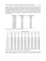
We define each membership function by obtaining upper and lower bounds of each
objective function. The upper and lower bounds obtained by maximizing and minimizing
each objective function separately are presented in Table 2.
6.2 Evaluation of results
As stated previously, we adopt the weighted additive approach proposed by Tiwari et al.
(1987) to deal with the collaborative CSCMP problem in a centralized SC structure. To