Supply Chain Management Pathways for Research and Practice Part 8 ppt

Information Sharing: a Quantitative Approach to a Class of Integrated Supply Chain

129
(m)Q/2
Q
m
/2
Q
1
/2
Q
0
/2
(m+1)Q/2
Q
m
/2
Q/2
Q
m-1
/2
0
t
s
t
Q
t
s+Q
t
2Q

Q/2
Q
m-2
/2
t
s+2Q
Q/2
t
mQ
Q
0

t
s+mQ
time

Each Supplier’s
inventory Position

Retailer’s inventory
Position
0
t
s
t
Q
t
s+Q
t
2Q

t
s+2Q
t
mQ
t
s+mQ
time

R
R+Q
R+s

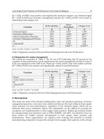
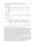
Fig. 5. Inventory position of the each supplier and the retailer in [
0, t
s
+ mQ]
In the same way it can be seen that the
j
th
unit in the batch Q
0
/2 (which will be received from
the path
i), will be used to fill the (R+j)
th
retailer demand after the retailer order. Then the j
th

unit in the batch
Q

0
/2 will have the same expected retailer and warehouse costs as a unit in a
base stock system with
S
0
=s+mQ and S
1
=R+j. Therefore the expected holding and shortage
costs for the
j
th
unit in the batch Q
0
/2 will be equal to c
i
(s+mQ, R+j), j=1,…, Q/2 (A(12)).
Similarly, one can easily see that the
j
th
unit in the batch Q
0
/2 (which will be received from
the path
j), will be used to fill the (R+Q/2+j)
th
retailer demand after the retailer order. Then
this unit will have the same expected retailer and warehouse costs as a unit in a base stock
system with
S
0

=s+mQ and S
1
=R+Q/2+j and the expected holding and shortage costs for this
unit will be equal to
c
j
(s+mQ , R+Q/2+j), j=1,…,Q/2 (A(12)).
It should be noted that each customer, demands only one unit of a batch. If we number the
customers who use all
Q units of these batches from 1 to Q, then the demand of any
customer will be filled randomly by one of these
Q units. That is, each unit of two batches of
(total)size
Q will be consumed by the j
th
( j=1,2,…,Q) customer according to a discrete
uniform distribution on
1,2,…,Q. In other words, the probability that the

i
th
(i=1,2,…,Q) unit
of two batches of (total)size
Q is used by the j
th
(j=1,2,…,Q) customer is equal to 1/Q.
Therefore we can now express the expected total cost for a unit demand as:

Supply Chain Management – Pathways for Research and Practice

130























2/
11)2/(
1221
2/
11)2/(
21

2
1
)),(),(.(
1
)),(),(.(
1
Q
i
Q
Qi
Q
i
Q
Qi
iRmQsciRmQscP
Q
iRmQsciRmQscP
Q
k

(17)

Since the average demand per unit of time is equal to
λ, the total cost of the system per unit
time can then be written as:




















2/
11)2/(
1221
2/
11)2/(
21
2
1
)),(),(.(
)),(),(.(.),,(
Q
i
Q
Qi
Q
i

Q
Qi
iRmQsciRmQscP
Q
iRmQsciRmQscP
Q
ksmRTC




(18)
Corollary: the probabilities P
ij
, are computed as follows: ( i, j = 1, 2, and P
ij
+ P
ji
= 1)
1: If L
1
> L
2
and L
0
1
> L
0
2
, then P

12
= 0.
2: If L
1
< L
2
and L
0
1
< L
0
2
, then P
12
= 1.
3: If L
1
> L
2
, L
0
1
< L
0
2
,

and L
1
+ L

0
1
< L
2
+ L
0
2
, then P
12
=G
s+mQ
(L
2
+ L
0
2
- L
1
), (B.1).
4: If L
1
> L
2
, L
0
1
< L
0
2
,

and L
1
+ L
0
1

> L
2
+ L
0
2
, then P
12
= 0.
5: If L
1
< L
2
, L
0
1
> L
0
2
, and L
1
+ L
0
1

> L
2
+ L
0
2
, then P
12
=G
s+mQ
(L
1
+ L
0
1
– L
2
).
6: If L
1
< L
2
, L
0
1
> L
0
2
, and L
1

+ L
0
1
< L
2
+ L
0
2
, then P
12
= 1.
One can find the idea of the proofs in appendix B and more information about this section in
(Sajadifar et. al, 2008).
5. Discussion
We, in model 1, derived the exact value of the total cost of the basic dyadic supply chain. In
model 2.1 and 2.2 we, using the idea introduced in model 1, obtained the exact value of the
expected total cost of the proposed inventory system. For demonstrating the effect of
information sharing, we define three different types of scenarios each of which derives the
benefits of sharing information between each echelon. Scenario 1: With Full information
sharing, scenario 2: With semi information sharing and scenario 3: Without information
sharing. For the first scenario, each echelon shares its online information to the upper
echelon, that is, s
1
and s
2
are both positive integer. With semi information sharing, just
echelon 1 shares its inventory position with echelon 2, then, only echelon 2 has online
information about the retailer′s inventory position, that is, s
1
is a positive integer and s

2
is
zero. And for the last kind of relation between echelons, we assume in third scenario, that
no echelon shares its online information about inventory position
that is the both value of s
1

and s
2
are zero. It means that we have no s
i
in this kind of relation. Numerical examples
show that the total inventory system cost reduces when the information sharing is on effect.
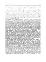
Table 1 consists of 6 pre-defined problems to show the IS effects.
Fig.6 shows the total cost of the inventory system for each problem and on each scenario. As
one can easily find, the more the information would be shared between echelons, the less
the total cost would be offered. Of course, from managerial point of view, the cost of

Information Sharing: a Quantitative Approach to a Class of Integrated Supply Chain

131
establishing information system must be considered for making any decision about sharing
information. The model presented in subsection 2.2 can enhance one to derive and
determine the exact value of shared information between each echelon.

Prob. No. Q λ β h
i
L
i

1 3 2 10 0.5 1
2 4 2 10 0.5 1
3 3 5 10 0.5 1
4 3 2 100 0.5 1
5 3 2 10 1 1
6 3 2 10 0.5 5
Table 1. Six Pre-Defined problems to show capability of three kinds of information sharing
policy in cost reduction


Fig. 6. Changing the
TC* in each scenario and in each problem.
In model 3, we expressed our findings as %deviation between average total cost rates
between the two systems, in which:
100%
nInformatioWith
nInformatioWith nInformatioWithout



TC
TCTC
deviation

For this purpose we fix all the parameters except λ, L
1
, L
2
and Q. These problems were
constructed by taking all possible combinations of the following values of the parameters

Q,
λ, L
1
, and L
2
: Q=2,6,10, 20; λ=2,5 ; L
1
, L
2
=0, 0.5, 1, 1.5 and 2. We have assumed that the value
of the parameters,
L
0
1
,L
0
2
,h , h
0
1
, h
0
2
and β are constant and for instance are as: 1,1 ,1 ,0.1 ,0.1
and 10 respectively.
These numerical examples show that the savings resulting from our policy will decrease as
the maximum possible lead time for an order increases. The value of information sharing
will be minimal when
Q is small or large. The most value of the shared information is 13%
saving in total cost for

λ=2, Q=10 and
0
()0.2
i
ii
LLL


.

Supply Chain Management – Pathways for Research and Practice

132
6. Conclusions
We, in this chapter, showed how to obtain the exact value of the total holding and shortage
costs for a class of integrated two-level inventory system with information exchange. Three
different models were introduced which incorporated the benefits of information sharing and
we, using the idea of the one-for-one ordering policy, obtained the exact value of the expected
total cost function for the inventory system in all of them. Resorting to some numerical
examples generated by model 2.2, we demonstrated that increasing the information sharing
between echelons of a serial supply chain can decrease the total integrated system costs. Also,
analyzing the findings of model 3, we showed that the savings resulting from our policy
decrease as the maximum possible lead time for an order increase, and the value of
information sharing will be maximal when the order size is neither large nor small.
7. Appendix A
This Appendix is a summary of Axsäter, S. (1990a). For more details one can see Axsäter, S.
(1990a)’s paper. We define (as in Axsäter, S. (1990a) for one retailer) the following notations:
)(
0
tg

S
Density function of the Erlang (
0
, S

)

and,
)(
0
tG
S
Cumulative distribution function of
)(
0
tg
S
.
Thus,

,
)!1(
)(
0
1
00
0
t
SS
S

e
S
t
tg







(A.1)
And,






0
0
!
)(
)(
Sk
t
k
S
e
k

t
tG



(A.2)

The average warehouse holding costs per unit is:

0)),(1())(1()(
00000
1
00
0
00


SLGLhLG
Sh
S
i
S
iii
S
i



(A.3)

And

for
0
0

S
,
.0)0(



(A.4)

Given that the value of the random delay at the warehouse is equal to
t, the conditional
expected costs per unit at the retailer is:

)()(
!
)(
)(
1
1
0
1
)(
1
1







S
tLtL
k
kS
h
et
i
S
k
kk
i
tL
S
i









(A.5)

Information Sharing: a Quantitative Approach to a Class of Integrated Supply Chain

133
( 0!=1 By definition),
The expected retailer’s inventory carrying and shortage cost to fill a unit of demand is:

)0())(1()()()(
1
0
0
1
0
1
0
0
0
0
0
0
S
i
S
L
S
i
S
S
LGdtttLgS
i





(A.6)

and,

)()0(
0
11
i
SS
L



(A.7)

Furthermore, for large value of
S
0
, we have

)0()(
11
0
SS
S




(A.8)

The procedure starts by determining
0
S such that


)(
0
0
LG
S

(A.9)

Where

is a small positive number.
The recursive computational procedure is:

)),0()0(())(1()()1(
1
00
1
0
11
0
11



SS
i
S
SS
LGSS


(A.10)



i
i
S
ii
S
L
S
LGLLGS





0
0
1
000

0
)()()(
00

(A.11)

and, The expected total holding and shortage costs for a unit demand in an inventory
system with a one-for-one ordering policy is:

)()(),(
0010
1
SSSSc
S
i



(A.12)

8. Appendix B
We will present the proof of the corollary 3 as follows:
iii
LX



,

and

},0max{
0 mQs
i
i
tL



,

then
)|().(
)|().(
)|().()(
2
021
2
0
2
0
1
021
2
0
1
0
1
021
1
02112

LtXXPLtP
LtLXXPLtLP
LtXXPLtPXXPP
mQsmQs
mQsmQs
mQsmQs








Supply Chain Management – Pathways for Research and Practice

134

)(
)()(
)()(
1
2
0212
1
0
1
2
0
2

1
02112
LLLGP
LGLLLG
LGXXPP
mQs
mQsmQs
mQs







(B.1)

All of the other corollaries can be proved easily in the same way.
9. References
Axsäter, S. (1990a). Simple solution procedures for a class of two-echelon inventory
problem.
Operations Research , Vol. 38, No. 1, pp. 64-69.
Axsäter, S. (1990b). Evaluation of (R,Q)-policies for two-level inventory systems with
Poisson demand.
Lulea University of Technology, Sweden.
Axsäter, S. (1993b). Exact and approximate evaluation of batch-ordering policies for two-
level inventory systems.
Operations Research , Vol. 41, No. 4, pp. 777-785.
Axsäter, S., Forsberg, R., & Zhang, W. (1994). Approximating general multi-echelon
inventory systems by Poisson models.

International Journal Production Economics ,
Vol. 35, pp. 201-206.
Cachon, G. P., & Fisher, M. (2000). Supply chain inventory management and the value of
shared information.
Management Science , Vol. 46, pp. 1032-1048.
Cheung, K. L., & Lee, H. L. (1998). Coordinated replenishments in a supply chain with
Vendor-Managed Inventory programs.
Working Paper.
Deuermeyer, B., & Schwarz, L. B. (1981). A model for the analysis of system seviece level in
warehouse/retailer distribution systems: The identical Retailer Case. in: L. B.
Schwarz (ed.),
Studies in Management Science, 16: Multi-level Production/Inventory
Control Systems, pp. 163-193.
Forsberg, R. (1995). Optimization of order-up-to-S policies for two-level inventory systems
with compound Poisson demand.
European Journal of Operational Research, Vol. 81,
pp. 143-153.
Forsberg, R. (1996). Exact evaluation of (R,Q)-policies for two-level inventory systems with
Poisson demand.
European Journal of Operational Research, Vol. 96, pp. 130-138.
Graves, S. C. (1985). A multi-echelon onventory model for a repairable item with one-for-
one replenishment.
Management Science, 31, pp1247-1256.
Gavirneni, S. (2002). Information flows in capacitated supply chains with fixed ordering
costs.
Management Science, Vol. 48, no. 5, pp. 644-651.
Gavirneni, S.; Kapuscinski, R. & Tayur, S. (1999). Value of information in capacitated supply
chains.
Management Science, Vol. 45, No. 1, pp. 16–24.
Hadley, G., & Whitin, T. M. (1963). Analysis of inventory systems. Prentice-Hall, Englewood

Cliffs, NJ.
Haji, R., Sajadifar, S. M., (2008), “Deriving the Exact Cost Function for a Two-Level
Inventory System with Information Sharing”,
Journal of Industrial and Systems
Engineering
, 2, 41-50.
Hajiaghaei-Keshteli, M. & Sajadifar, S. M. (2010). Deriving the cost function for a class of
three-echelon inventory system with N-retailers and one-for-one ordering policy.
International Journal of Advanced Manufacturing Technology, Vol. 50, pp. 343-351.
Hajiaghaei-Keshteli, M.; Sajadifar, S. M. & Haji, R. (2010). Determination of the economical
policy of a three-echelon inventory system with (R, Q) ordering policy and

Information Sharing: a Quantitative Approach to a Class of Integrated Supply Chain

135
information sharing. International Journal of Advanced Manufacturing Technology,
DOI: 10.1007/s00170-010-3112-6.
Hsiao, J. M., & Shieh, C. J. (2006). Evaluating the value of information sharing in a supply
chain using an ARIMA model. International Journal of Advanced Manufacturing
Technology
, Vol. 27, pp. 604-609.
Kelepouris, T., Miliotis, P. and Pramatari, K. (2008). The Impact of Replenishment
Parameters and Information Sharing on the Bullwhip Effect: A Computational
Study. Computers and Operations Research, 35, pp3657-3670
Kelle, P. & Silver, E.A. (1990a). Safety stock reduction by order splitting. Naval Research
Logistics
, Vol. 37, pp. 725–743.
Kelle, P. & Silver, E.A. (1990b). Decreasing expected shortages through order splitting.
Engineering Costs and Production

Economics, Vol. 19, pp. 351–357.
Lee, H. L.; So K. C. & Tang C. S. (2000). The value of information sharing in a two-level
supply chain.
Management Science, Vol. 46, No. 5, pp. 626–643.
Lee, H. L., & Moinzadeh, K. (1987a). Two-parameter approximations for multi-echelon
repairable inventory models with batch ordering policy.
IIE Transactions, Vol. 19,
pp. 140-149.
Lee, H. L., & Moinzadeh, K. (1987b). Operating characteristics of a two-echelon inventory
system for repairable and consumable items under batch ordering and shipment
policy.
Naval Research Logistics Quarterly, Vol. 34, pp. 356-380.
Lee, H. L., & Whang, S. (1998). Information sharing in a supply chain.
Working Paper.
Milgrom, P., & Roberts, J. (1990). The economics of modern manufacturing technology:
strategy and organization
. American Economic Review, Vol. 80, pp. 511-528.
Moinzadeh, K. (2002). A multi-echelon inventory system with information exchange.
Management Science, Vol. 48, No. 3, pp. 414-426.
Moinzadeh, K., & Lee, H. L. (1986). Batch size and stocking levels in multi-echelon
repairable systems.
Management Science, Vol. 32, pp. 1567-1581.
Presutti, W. D. (1992). The single sourcing issue: US and Japanese sourcing strategies.
International Journal of Purchasing and Materials Management, pp. 2-9, 1992.
Ramasesh, R. V.; Ord, J. K.; Hayya J. C. & Pan, A. C. (1991). Sole versus dual sourcing in
stochastic lead-times, Q inventory
models. Management Science, Vol. 37, No. 4, pp.
428–443.
Sajadifar, S.M, ; Hendi, A. M & Haji, R. (2008). Exact Evaluation of a Two Sourcing Supply
Chain with Order Splitting and Information Sharing,

The IEEE International
Conference on Industrial Engineering and Engineering Management,
pp. 1835-1839.
Sculli, D. & Shum, Y.W. (1990). Analysis of a continuous review stock-control model with
multiple suppliers.
Journal of

the Operational Research Society, Vol. 41, No. 9, pp. 873–
877.
Sculli, D. & Wu, S. Y. (1981). Stock control with two suppliers and normal lead times.
Journal
of the Operational Research

Society, Vol. 32, pp. 1003–1009.
Sedarage, D.; Fujiwara, O. & Luong, H. T. (1999). Determining optimal order splitting and
reorder levels for n-supplier inventory systems.
European Journal of Operational
Research
, Vol. 116, pp. 389–404.
Seifbarghi, M., & Akbari, M. R. (2006). Cost evaluation of a two-echelon inventory system
with lost sales and approximately Poisson demand.
International Journal of
Production Economics
, Vol. 102, pp. 244-254.

Supply Chain Management – Pathways for Research and Practice

136
Sherbrooke, C. C. (1968). METRIC: A multi-echelon technique for recoverable item control.
Operations Research, Vol. 16, pp. 122-141.

Svoronos, A. & Zipkin, P. (1988). Estimationg the performance of multi-level inventory
systems.
Operations Research, Vol. 36, pp. 57-72.
Thomas, D. J. & Tyworth, J. E. (2006). Pooling lead-time risk by order splitting: A critical
review.
Transportation Research Part E, Vol. 42, pp. 245–257.
Xiaobo, Z. and Minmin, Q. (2007). Information sharing in a Multi-Echelon Inventory
System.
Tsinghua Science and Technology, 12, 4, pp466-474.
Yao, D. Q.; Yue, X. ; Wang X.; & Liu, J. J. (2005). The impact of information sharing on a
returns policy with the addition of a direct channel.
International Journal Production
Economics
, Vol. 97, pp. 196–209.
10
Production and Delivery Policies for Improved
Supply Chain Performance

Seung-Lae Kim and Khalid Habib Mokhashi
Decision Sciences Department, LeBow College of Business, Drexel University,
Philadelphia
USA
1. Introduction

The research on supply chain management evolved from two separate paths: (1) purchasing
and supply perspective of the manufacturers, and (2) transportation and logistics
perspective of the distributors. The former is the same as supplier base integration, which
deals with traditional purchasing and supply management focusing on inventory and cycle
time reduction. The latter concentrates on the logistics system for effective delivery of goods
from supplier to customer. Supply chain management focuses on matching supply with

demand to improve customer service without increasing inventory by eliminating
inefficiencies and hidden operating costs throughout the whole process of materials flow.
An essential concept of supply chain management is thus the coordination of all the
activities from the material suppliers through manufacturer and distributors to the final
customers. Recently, many researchers (for example, Weng, 1997, Lee and Whang, 1999,
Cachon and Lariviere, 2005, Gerchak and Wang, 2004, Davis and Spekman, 2004, Yao and
Chiou, 2004, Chang et al., 2008 among others) have examined theoretical, as well as
practical, issues involving buyer-supplier coordination. The research findings claim that
well coordinated supply chains have the potential for companies competing in a global
market to gain a competitive advantage, especially in situations involving outsourcing,
which is becoming increasingly common.
The current chapter discusses, from the perspective of supplier base integration, supply
chain coordination for a make-to-order environment in which manufacturing (or assembly)
and shipping capacity is ready. The managers have purchase orders in hand and the choice
of flexible production and delivery policies in filling the order. For the benefits of
operational efficiency, the supplier adopts the policy of frequent shipments of manufactured
parts and products in small lots. In the case of standard-size container shipping, each
container has limited space, and the manufacturer should split the orders into multiple
containers over time. This can be extended to the situation where the manufacturer may
have to use multiple companies (different trucks) to ship the entire orders. For the buyer, it
is important to work closely with the supplier to facilitate frequent delivery schedules so
that the supplier is able to meet the buyer’s requirements while still remaining economically
viable. Obviously, this collaboration is an example of vendor managed inventory (VMI)
system that requires well-managed cooperation between buyer and supplier in terms of

Supply Chain Management – Pathways for Research and Practice
138
sharing information on demand and inventory. While using the multiple delivery models, it
is assumed that the vendor has the flexibility to select its own production policy. It can
produce all units in a single setup or multiple setups to respond to a buyer’s order. The

existing literature, however, has not focused on comparisons between single-setup-multiple-
delivery (SSMD) and multiple-setup-multiple-delivery (MSMD) policies. Although the
SSMD policy is well accepted and gaining popularity, the MSMD policy has been largely
disregarded due to the likelihood of high setup costs. However, when we factor in setup
reduction through learning and the reduction of necessary inventory space, the MSMD may
be just as viable, or even the better option in certain situations. For example, suppose in a
make-to-order environment that the supplier receives customer orders frequently through
the Internet and has cost/time efficient setup operation, then it is natural for the supplier to
choose the MSMD policy over the SSMD policy, since the MSMD policy would help the
company keep a low inventory and provide fast delivery to its customers, obviously
enhancing the supplier’s competitive advantage. This advantage will be apparent especially
for the companies in high tech industries, where the product’s life cycle tends to be shorter.
This is also true of companies in the food industry, where the demand is always for fresh
products. See David Blanchard, 2007 for more examples.
In this study, we extend the models that focused on the supplier’s production policy (See
Kim et al., 2008, and Kim and Ha, 2003). Kim et al., 2008 assumed in their MSMD model that
the setup reduction through learning is restricted to one single lot and the learning starts
anew for the next lot. In our first extension, however, we relax that assumption and allow
that the setup reduction through learning is continued and accumulated throughout the
subsequent production lots. The second extension of the model is that the MSMD model is
allowed to have unequal setups and deliveries, while retaining the assumption of the
MSMD model that the learning on setup reduction is confined to each lot alone and does not
continue across lots. In other words, the model allows the number of setups to be unequal to
the number of deliveries in each lot. This model may provide greater flexibility to the
supplier in determining the production policy compared to the MSMD model or the SSMD
model. Numerical examples are presented for illustration.
Although our goal is to elaborate on the entire supply chain synchronization, our discussion
is limited to a relatively simple situation, i.e., single buyer and single supplier, under
deterministic conditions for a single product that may account for a significant portion of
the firm's inventory expenses. It is hoped that the result can be extended to a supply chain

where multiple products and multiple parties are involved. In the following sections, the
chapter discusses the supply chain coordination issue, from the perspective of supplier base
integration, for a make-to-order environment in which manufacturing (or assembly) and
shipping capacity is ready. The supplier has the flexibility to select its own production
policy, producing all units of demand in either a single setup or multiple setups to respond
to a buyer’s order, and also to choose a shipping policy of single or multiple deliveries for a
given lot. Not much research in the existing literature has focused on comparisons between
single-setup-multiple-delivery (SSMD) and multiple-setup-multiple-delivery (MSMD)
policies. This study compares the SSMD and the MSMD policies, where frequent setups give
rise to learning in the supplier's setup operation. A multiple delivery policy shows a strong
and consistent cost-reducing effect on both the buyer and the supplier, in comparison to the
traditional lot-for-lot approach. This paper extends the MSMD model in two directions: (1)
Modified MSMD Model (I): multiple-setup-multiple-delivery with allowance for unequal
number of setups and deliveries, and (2) Modified MSMD Model (II): multiple-setup-

Production and Delivery Policies for Improved Supply Chain Performance
139
multiple-delivery with allowance for cumulative learning on setups over the subsequent
production cycles. Numerical illustrations are provided to compare the performance of the
proposed models. The concluding section summarizes and discusses the implications of the
results obtained.
2. Assumptions of the models and notation
When the buyer orders a quantity, Q, the supplier in response can pursue one of the
following three policies: (1) Lot for Lot, i.e., single-setup-single-delivery (SSSD), (2) SSMD,
or (3) MSMD. In the latter two cases, the order quantity, Q, will be split into a smaller
delivery size over multiple deliveries, while the setup frequency for each policy would be
different. If the setup cost is relatively high, a less frequent setup may be economically
attractive to the supplier. The supplier would prefer to produce the entire order quantity, Q,
with one setup, unless it can reduce the setup cost significantly to justify multiple setups. In
this SSMD case, the supplier will hold and maintain the buyer's inventory due to the small

delivery lot size. And because the supplier has all the necessary information, he often
assumes the role of a central decision-maker in a vendor-managed inventory system. The
supplier's cost function includes a setup and order handling cost, and a holding cost, while
the buyer's relevant costs consist of an ordering cost, a variable holding cost, and a fixed
transportation cost. However, it is not unusual for the buyer to pay increased order
handling costs because it is incurred as a result of frequent deliveries imposed by the buyer.
If the MSMD policy is chosen, on the other hand, the supplier can meet the buyer’s demand
with lower inventories than in the case of the SSMD policy. But he will incur higher setup
costs due to more frequent setups. Also, there will be opportunity costs for the supplier that
account for the capacity foregone by having more frequent setups than with the SSMD
policy for a given order quantity. However, the MSMD policy may give rise to learning
effects on setup operations, which in turn will reduce setup time and cost. The reduced
setup time (and cost) will eventually benefit the supplier in the long run. It is reasonable for
the buyer and the supplier to share this opportunity cost, because both the buyer and
supplier can benefit from such a policy: the supplier achieves setup reduction via the
learning effect on setup operations, and the buyer receives the benefits of multiple
deliveries, i.e., lower inventories.
Once a long-term contract between buyer and supplier is agreed upon, both parties work in
a cooperative manner to coordinate supply with actual customer demand. Their effective
linkage in this manner will eventually make any practice of frequent delivery in small lot
sizes beneficial to both parties. In this study, market demand rate, production rate, and
delivery time are assumed to be constant and deterministic. It is also assumed that all cost
parameters, including unit price, are known and constant, and neither quantity-discount nor
backorders are allowed. The following notations are adopted:
A = the ordering cost per order for buyer,
a = a parameter associated with supplier's hourly opportunity cost,
b = a parameter associated with decreasing rate of setup time, -ln r / ln 2 where r
represents the percentage learning rate for the supplier’s setup operations,
C = the supplier's hourly setup cost,
D = the annual demand rate for buyer,

F = the fixed transportation cost per delivery trip,
H
B

= the holding cost/unit/year for buyer,

Supply Chain Management – Pathways for Research and Practice
140
H
S
= the holding cost/unit/year for supplier, H
B

> H
S

J = the number of supplier setups per customer lot order, J = 1, 2, 3,…., N,
K = the supplier’s hourly opportunity cost for the time foregone attributed to the increased
number of setups,
N = the number of deliveries per production cycle,
P = the annual production rate for supplier, P > D,
Q = the order quantity for buyer,
q = the delivery lot size per trip, q = Q/N,
S = the setup time/setup for supplier,
V = the unit variable cost for order handling and receiving,
 = the proportion of the fixed part of the total setup cost,
m = the number of deliveries per setup within a production cycle.
3. Single-Setup-Multiple-Delivery (SSMD) model
In the SSMD model, the order quantity is produced with one setup and shipped through
multiple deliveries over time. The multiple deliveries are to be arranged in such a way that

each succeeding delivery arrives at the time that all inventories from the previous delivery
have just been depleted. As mentioned earlier, the buyer's total cost consists of ordering and
holding costs, as well as transportation costs, incurred during the multiple deliveries as:

(, ) ( )
2
Buyer B
DQ DN Q
TC Q N A H F V
QN Q N
  
(1)
And the supplier's cost function includes a setup and order handling cost, and a holding
cost:

(, ) (2 ) 1
2
S
Supplier
QH
DD
TC Q N CS N N
QN P








(2)
The aggregate total cost function for both parties is as follows:
Note that N = 1 reduces Equations (1) – (3) to the conventional single delivery case, which is
a special case of the SSMD
(,) ( ) (2 ) 1 ( )
2
Aggregate B S
DQ D DNQ
TC Q N A CS H H N N F V
QN P QN


   




(3)
policy. The fact that the second derivatives of Equation (3) (with respect to Q and N) are
positive confirms the convexity of the aggregated total cost function. The optimal contract
quantity, delivery frequency, and delivery size are as follows:
*
2( )
(1 )
SSMD
S
DA CS
Q
D
H

P




*
(){( )2}
()
BS S
S
ACSPH H DH
N
FP DH





Production and Delivery Policies for Improved Supply Chain Performance
141

2
*
()2
DFP
q
PH H DH
BS S



(4)
The expression for optimal order (contract) quantity for SSMD is almost identical to the
supplier’s independent Economic Production Quantity (EPQ) model, except that the
buyer’s ordering cost, A, is added to the supplier’s setup cost in the numerator of
Equation (4). In the SSMD model, the buyer’s holding costs and transportation costs do
not affect the contract quantity. In other words, the supplier can determine the contract
quantity alone without the knowledge of the buyer’s holding and transportation costs
information. In fact, the integrated optimal order quantity in Equation (4) is greater than
the supplier’s independent production quantity by the ratio of
(1 )
A
CS
 , which is close to
1 when the buyer’s order cost, A, is very low compared to the supplier’s setup cost, CS, as
the case may be in current applications of electronic data interchange (EDI) based
ordering systems in JIT environments. This is one of the reasons why the supplier may be
willing to take a leading role in establishing such supplier-buyer linkage. The optimal
delivery size is obtained by dividing the order quantity by the number of deliveries in
Equation (4). Kim and Ha, 2003 claimed that the SSMD policy consistently outperforms
the single delivery policy, given that the order quantity is greater than the minimum
required level.
4. Multiple-Setup-Multiple-Delivery (MSMD) model
In the SSMD model, as shown in the earlier section, the supplier maintains large inventories
and incurs high inventory holding costs due to the small delivery lot sizes over the multiple
shipments. If the supplier, however, chooses the MSMD policy to set up the production
process more frequently and to produce the exact quantity to be shipped on every setup, it
can meet the buyer’s demand with lower average inventory than in the case of the SSMD
policy. But the supplier in this MSMD case consumes more capacity hours due to frequent
setups, which incurs higher setup costs in the long run. However, if the supplier’s capacity
is greater than the threshold level (P = 2D), it is more beneficial for the supplier to

implement the MSMD policy, even though he pays more frequent setup costs since the
savings in inventory holding costs is greater than the increased setup costs. The supplier
who has a tight constraint on capacity, therefore, should not choose the MSMD policy until
its capacity is expanded. If the supplier has no constraint on capacity, or the savings earned
from the lowered inventories compensate for the opportunity costs of the foregone capacity,
the MSMD policy would be a feasible option to implement. One other factor pertaining to
the MSMD policy is that the MSMD policy results in an increased opportunity to achieve
larger learning effects on setup operations, which, in turn, will reduce the setup time/cost.
In the following, we develop the structure of the MSMD policy and compare it with the
SSMD policy in order to help the decision maker choose the appropriate policy for a given
supply chain environment.
We now assume that the system has no constraint on capacity for setting up N batches to
produce the order quantity, i.e., the order quantity, Q, is equally split, manufactured and
delivered over N times. Learning effects on setup operations is also assumed to reduce the
setup time/cost per setup, as the number of setups increases. The MSMD policy obviously

Supply Chain Management – Pathways for Research and Practice
142
changes the supplier's cost structure significantly, but the buyer’s total cost remains intact as
in Equation (1). The supplier's total cost consists of the setup cost that reflects learning
effects due to multiple setups, the holding cost, and the opportunity cost that accounts for
the extra setups in the supplier's capacity. The following equation shows these costs in
order:


/
1
/
(1)
1

(, ) (1 )
2
1 ( 1) (1 ) , 2.
DN Q
b
S
Supplier
J
DN Q
aN
b
D
J
Q
QH
DD
TC Q N CS N J
QNP
D
Ke S N J N
Q










 







 






(5)
In Equation (5) above, α is the fixed cost portion of the setup cost. The setup cost has two
components: fixed (or machine) and variable (or human) setup operation. And the learning
effect is applied to the variable setup cost only. Without multiple setups, i.e., if N=1,
Equation (5) reduces to the conventional single delivery lot-for-lot model. The second term
in Equation (5) depicts the holding costs, and the third term represents the opportunity cost
for the capacity foregone due to increased setups. Frequent setups are more likely to disrupt
the supplier's current production schedule and thus there would be opportunity costs for
the capacity foregone by having more frequent setups than an SSMD policy. As the number
of setups, N, increases, the supplier's current opportunity cost per unit time, K, also
increases. This increasing pattern can be modeled by one of various possible functions, such
as linear or exponential, depending upon the supplier's situation of capacity available. If a
vendor operates a tight production schedule, the initial opportunity cost (K) and the
increasing rate of cost per unit of time will be higher than those of other vendors with a less
tight schedule. In this paper, the unit time opportunity cost is assumed to be exponentially

increasing as shown in the first part of the last term of Equation (5). The second part of the
term, which reflects learning effects, is the amount of the supplier's capacity used up for
increased number of setups. The entire term then represents the opportunity cost per unit of
time. Note that this opportunity cost term vanishes when N=1.
The integrated total cost function for both parties is as shown below:


/
1
/
(1)
1
(, ) (1 )

2
1 ( 1) (1 ) ,
DN Q
b
Aggregate
J
BS
DN Q
aN
b
D
J
Q
DD
TC Q N A CS N J
QQ

QDDNQ
HH FV
NPQN
D
Ke S N J
Q









 










 







2,N 
(6)
Since the terms reflecting learning effects in Equation (6) bring step functions into the
equation, derivatives with respect to Q and N do not exist at the boundary points of each J.
Therefore we approximate Equation (6) by a continuous function, i.e.,

Production and Delivery Policies for Improved Supply Chain Performance
143

0.5
0.5
(1
(, ) (1 )

2

D
N
Q
b
Aggregate
J
BS
aN
DD
TC Q N A CS N J dJ
QQ

QDDNQ
HH FV
NPQN
Ke








 











0.5
)
0.5
1 ( 1) (1 ) , 2,
D
N

Q
b
D
J
Q
D
SN JdJN
Q








 





(7)
Integration for J in Equation (7) leads to
1
1
(1 )
(, ) 0.5 0.5
(1 )

2

b
b
Aggregate
BS
DD D
TC Q N A CS N N
QQbQ
QDDNQ
HH FV
NPQN










   














11
(1)
(1 )
1 ( 1) 0.5 0.5 .
(1 )
bb
aN
DDD
Ke S N N
QbQ Q















  












(8)
If the MSMD policy is chosen, the supplier can meet the buyer’s demand with lower
inventories than in the case of the SSMD policy, although more frequent setups will incur
higher setup costs. A comparison of the integrated total costs for both SSMD and MSMD
policies in Equations (3) and (8) would be sufficient in leading the supplier to an informed
decision. However, since it is difficult to make an algebraic comparison of the two total costs
due to the complexities of the expressions, Kim et al., 2008 suggested a brief guideline to
help the supplier in making a decision about setup and delivery policy: If the supplier’s
capacity is greater than the threshold level (P = 2D), it is more beneficial for the supplier to
implement the MSMD policy and to maintain fewer inventories. Even though the supplier
pays greater costs for the frequent setups compared to the SSMD policy, the savings in
inventory holding costs surpasses the increased setup costs. As the supplier’s production
capacity increases, MSMD becomes more and more cost effective. On the other hand, the
smaller the supplier’s production capacity, the more beneficial SSMD becomes. When we
take the learning effect on setup operation into our consideration, as the learning rate on
setup operation increases, the rate at which MSMD becomes more efficient accelerates. In
the next two subsections, we discuss the extensions of the MSMD model.

4.1 Modified MSMD model (I): Unequal number of setups and deliveries
In this section, we develop a modified multiple setup multiple delivery model (modified
MSMD Model (I)), which retains the assumption that the setup reduction through learning
is confined to each lot alone and does not continue across lots. However, the modified
MSMD model (I) proposed in this section allows the number of setups to be unequal to the
number of deliveries in each lot. This model may provide greater flexibility to the supplier
in determining the production and delivery policy compared to the MSMD model. For

Supply Chain Management – Pathways for Research and Practice
144
certain parameter values, this modified MSMD model (I) will result in lower total cost
compared to the MSMD model. In our modified MSMD model (I) with unequal setups and
deliveries, the total cost function takes the following form:


1
1
(1 )
(,,) 0.5 0.5
(1 ) 2
N
2 1
m2
b
b
Agg
re
g
ate B
S

DDN DN Q
TCQmN A CS H
QQmbQm N
QDDNQ
Hmm FV
mPQN









 

    


 


 




    



  
    

11
(1)

(1 )
1 ( 1) 0.5 0.5 .
(1 )
bb
N
a
m
DN D N D
Ke S
Qm b Q m Q
















  














(9)
In this modified MSMD model (I), m is the number of deliveries per setup within a
production cycle. The aggregate total cost is comprised of the ordering cost, the setup cost,
the inventory cost for both the supplier and the buyer, transportation cost, and the
opportunity cost owing to additional setups within the production cycle. The frequency of
setups within a production cycle is defined in this model as the ratio of the total number of
deliveries to the number of deliveries per setup in a production cycle. The model is
formulated as a mixed integer nonlinear programming problem with the objective to
minimize the total cost and determine the optimal production batch quantity (Q), optimal
number of deliveries (m) per setup, and optimal number of deliveries (N) per production
cycle. The constraints for the model are that all three variables Q, m, and N are greater than
0, that N is an integer, and that the number of orders in the finite planning period times the
optimal order quantity per batch equals the demand for that finite planning period. The

production batch quantity is less than or equal to the demand during the finite planning
period, and frequency of setups within a production cycle is greater than 0. The
mathematical formulation of the mixed integer nonlinear programming problem for the
proposed model is formulated below:
Minimize:


1
1
(1 )
(,,) 0.5 0.5
(1 ) 2
N
2 1
m2
b
b
Agg
re
g
ate B
S
DDN DN Q
TCQmN A CS H
QQmbQm N
QDDNQ
Hmm FV
mPQN










 

    


 


 




    


  
    

11
(1)

(1 )

1 ( 1) 0.5 0.5 .
(1 )
bb
N
a
m
DN D N D
Ke S
Qm b Q m Q















  















(10)
Subject to:
Q, m, N > 0,
N and m are integers,
,
D
QD
Q





Q
 D,

Production and Delivery Policies for Improved Supply Chain Performance
145
1.
N
m






4.2 Modified MSMD model (II): Cumulative learning on setups over production cycles
In this section, we propose another extension of the MSMD model, which allows the learning
of setup reduction achieved through earlier operations to accumulate across production cycles
throughout the entire planning period. When this is imposed on the modified MSMD model
(I), the model becomes modified MSMD model (II), which has the dual properties of both the
SSMD and the MSMD models. This model can be applied to the situation where the time
interval between consecutive orders is short enough for the supplier not to lose the learning
gained from earlier setup operations. The model is thus built along the lines of single setup
multiple deliveries with learning on setups over the multiple cycles. The benefits of this model
over the MSMD model may be twofold: First, the overall setup cost and, in turn, the total cost
is lower compared to the MSMD model. Second, the opportunity cost component incurred
owing to additional setups in the MSMD model can be eliminated since the setup times are
reduced as the production cycle is repeated. This, in turn, increases the scope for further
reduction in the total cost for the same parameter values compared to the MSMD model. The
total cost function takes the following form:

1
1
(1 )
(, ) 0.5 0.5
(1 )
(2 ) 1
22
b
b

Aggregate
S
B
DD D
TC Q N A CS
QQbQ
QH
QDDNQ
HNNFV
NN P QN










   










 


(11)
In this model, the total cost is comprised, as shown above, of the ordering cost, the setup
cost that reduces through learning for subsequent setups during the entire finite planning
period, the inventory cost of the buyer and the supplier, and the transportation cost, which
is comprised of the fixed and the variable transportation cost components. The model is
built along the lines of the single setup multiple delivery models with the addition of the
variable N, the number of shipments from the supplier to the buyer in each setup. Owing to
multiple shipments during each production lot, the supplier’s inventory cost function is
similar to the one obtained by Kim and Ha (2003).
The modified MSMD model (II) can be formulated as a mixed integer nonlinear
programming problem with the objective to minimize the total cost as shown below:
Minimize:

1
1
(1 )
(, ) 0.5 0.5
(1 )
(2 ) 1
22
b
b
Aggregate
S
B
DD D
TC Q N A CS

QQbQ
QH
QDDNQ
HNNFV
NN P QN










   









 


(12)
Subject to:

.
D
QD
Q






Supply Chain Management – Pathways for Research and Practice
146
The variables to be determined are the production batch quantity Q and the number of
shipments N in order to determine the supplier’s production and delivery policy at the
minimal total cost for the supply chain.
5. Numerical illustration
Suppose a buyer, who is currently using an EOQ policy seeking short-term advantage, plans
to develop a long-term buyer-vendor relationship for an improved supply chain
management. The buyer's annual demand is D = 4,800 units/year, ordering cost is A =
$25/order, and holding cost is H
B
= $5/unit/year. The fixed cost per trip and unit variable
transportation costs are F = $50.00 and V = $1.00/unit, respectively. For our illustration
purposes, we consider that the supplier's annual production capacity can be any level of the
following: 9,600 units, 19,200 units, 28,800 units, 38,400 units, and 48,000 units. Depending
upon the supplier’s selected capacity level, the supplier may use from 50% to 10% of its
capacity to meet the buyer’s demand. The unit holding cost for the supplier, H
S
=
$4/unit/year. It currently takes 5 workers 6 hours to set up the system, and the hourly labor

cost per worker is $20. Thus, the cost per setup is $600 ($20/hr × 5 worker × 6 hrs.). And the
fixed cost portion of the setup cost (α) is 0.5. The learning rates (r) considered in this
example are 90% (b = 0.152003), 80% (b = 0.321928), and 70% (b = 0.514573). The parameter
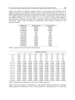
value associated with the supplier’s hourly opportunity cost (a) is 0.003. Tables 2 through 16
illustrate 15 different scenarios, in which only the production rate (P) and the learning rate
(r) vary while other parameters remain unchanged. Notice that the parameter (b), which is
associated with the learning rate, varies as the learning rate varies.



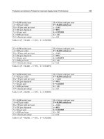
D = 4,800 units/year H
S
= $4 per unit per year
A = $25 per order
P = 9,600 units/year
H
B
= $5 per unit per year
a
F = $50 per shipment
r = 90%
V = $1 per unit
b = 0.152003
C = $100 per hour K = 100
S = 6 hours per setup
 = 0.5
Table 2. (P = 9,600, r = 90%, b = 0.152003)

D = 4,800 units/year H
S
= $4 per unit per year
A = $25 per order
P = 9,600 units/year
H
B
= $5 per unit per year
a
F = $50 per shipment
r = 80%
V = $1 per unit
b = 0.321928
C = $100 per hour K = 100
S = 6 hours per setup
 = 0.5
Table 3. (P = 9,600, r = 80%, b = 0.321928)

Production and Delivery Policies for Improved Supply Chain Performance
147



D = 4,800 units/year H
S
= $4 per unit per year
A = $25 per order
P = 9,600 units/year
H
B

= $5 per unit per year
a
F = $50 per shipment
r = 70%
V = $1 per unit
b = 0.514573
C = $100 per hour K = 100
S = 6 hours per setup
 = 0.5
Table 4. (P = 9,600, r = 70%, b = 0.514573)



D = 4,800 units/year H
S
= $4 per unit per year
A = $25 per order
P = 19,200 units/year
H
B
= $5 per unit per year
a
F = $50 per shipment
r = 90%
V = $1 per unit
b = 0.152003
C = $100 per hour K = 100
S = 6 hours per setup α = 0.5
Table 5. (P = 19,200, r = 90%, b = 0.152003)

D = 4,800 units/year H
S
= $4 per unit per year
A = $25 per order
P = 19,200 units/year
H
B
= $5 per unit per year
a
F = $50 per shipment
r = 80%
V = $1 per unit
b = 0.321928
C = $100 per hour K = 100
S = 6 hours per setup
= 0.5
Table 6. (P = 19,200, r = 80%, b = 0.321928)


D = 4,800 units/year H
S
= $4 per unit per year
A = $25 per order
P = 19,200 units/year
H
B
= $5 per unit per year
a
F = $50 per shipment

r = 70%
V = $1 per unit
b = 0.514573
C = $100 per hour K = 100
S = 6 hours per setup


Table 7. (P = 19,200, r = 70%, b = 0.514573)

Supply Chain Management – Pathways for Research and Practice
148



D = 4,800 units/year H
S
= $4 per unit per year
A = $25 per order
P = 28,800 units/year
H
B
= $5 per unit per year
a
F = $50 per shipment
r = 90%
V = $1 per unit
b = 0.152003
C = $100 per hour K = 100
S = 6 hours per setup
= 0.5

Table 8. (P = 28,800, r = 90%, b = 0.152003)



D = 4,800 units/year H
S
= $4 per unit per year
A = $25 per order
P = 28,800 units/year
H
B
= $5 per unit per year
a
F = $50 per shipment
r = 80%
V = $1 per unit
b = 0.321928
C = $100 per hour K = 100
S = 6 hours per setup
= 0.5
Table 9. (P = 28,800, r = 80%, b = 0.321928)


D = 4,800 units/year H
S
= $4 per unit per year
A = $25 per order
P = 28,800 units/year
H
B

= $5 per unit per year
a
F = $50 per shipment
r = 70%
V = $1 per unit
b = 0.514573
C = $100 per hour K = 100
S = 6 hours per setup


Table 10. (P = 28,800, r = 70%, b = 0.514573)


D = 4,800 units/year H
S
= $4 per unit per year
A = $25 per order
P = 38,400 units/year
H
B
= $5 per unit per year
a
F = $50 per shipment
r = 90%
V = $1 per unit
b = 0.152003
C = $100 per hour K = 100
S = 6 hours per setup
 0.5
Table 11. (P = 38,400, r = 90%, b = 0.152003)