Wiley Wastewater Quality Monitoring and Treatment_14 ppt

JWBK117-3.4 JWBK117-Quevauviller October 10, 2006 20:30 Char Count= 0
236 Nutrient Control
by the carrier; thus, in sulfamic acid only nitrate is reduced and in water nitrate and
nitrite. Photoreduction has been also used with biamperometric detection (Gil-Torro
et al., 1998), detecting the triiodide formed by reaction between iodide and nitrite. As
previously mentioned two measurements should be performed, with and without ir-
radiation in order to achieve speciation. Exclusive detection of nitrate is uncommon,
however, methods with electrochemical detection have been proposed for this pur-
pose. Thus, for example, the coulometric determination of nitrate by reduction over
a glassy carbon electrode, without interference of oxygen or nitrite (Nakata et al.,
1990) has been proposed or the potentiometric determination by means of photo-
cured coated-wire electrodes in the flow injection potentiometric mode (Alexander
et al., 1998). However, it should be mentioned that only the potentiometric deter-
mination has been applied in the analysis of wastewater samples. In Table 3.4.1
the analytical characteristics of some of the above-mentioned methods can be also
observed.
Organic and total nitrogen
For organic nitrogen determination sample digestion is required to transform the
organic compounds containing nitrogen into nitrogen inorganic species. From the
mineralized sample the total nitrogen content can be determined and by subtraction
the organic nitrogen content. Sample digestion is the most tiresome and slowest step
of the analysis process of these parameters and, hence, has deserved greater atten-
tion as far as researchers are concerned with the aim to achieve its automation. This
digestion can be carried out in different ways, namely: Kjeldahl method, photochem-
ical oxidation, alkaline oxidation with persulfate or combustion at high temperature.
The Kjeldahl method is the recommended manual standard method and provides
a parameter widely used in water characterization, the so-called Kjeldahl nitrogen.
Although several flow methods may be found in the literature based on segmented
flow designs, where digestion is carried out in a helicoidal reactor at controlled tem-
perature (Davidson et al., 1970), the metallic catalyser has been substituted by a
sulfonitric mixture and the on-line detection is carried out by the Berthelot reaction;

however, these methods have not been applied to wastewater samples. The main
problems hampering the implementation of the digestion step in the case of waste-
water samples are the obstruction of the flow channels in the digester together with
the low recoveries attained. Due to the former reasons, the habitual analysis of this
parameter in wastewaters is proposed to be performed by semiautomatic methods,
whereby digestion is carried out in traditional digesters and the treatments and/or
developments of the reaction for the detection in flow systems (Cerd`a et al., 2000).
Besides, if automation of the distillation step is aimed for, the difficulty increases
considerably and, thus, many researchers have looked for alternatives other than the
popular Kjeldahl method. One of these alternatives is on-line UV-photooxidation
in the presence of oxidizing agents such as hydrogen peroxide or potassium per-
sulfate. Through this treatment organic nitrogen and ammonium are converted into
JWBK117-3.4 JWBK117-Quevauviller October 10, 2006 20:30 Char Count= 0
Flow Analysis Methods 237
D
Resin
W
DB
SV1
Thermostatic
bath (40 °C)
Photoreactor
Sample
ml/ min
0.20
0.36
0.36
1.2
RC1
RC2

W
IV
SV2
1.2
1.2
R1
R2
R3
H
2
O
H
2
O
Sample
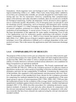
Figure 3.4.2 Flow injection arrangement for determination of nitrite, nitrate and total nitrogen.
R1, peroxydisulfate alkalinesolution; R2,reducing agent;R3, chromogenic reagent; Resin, amber-
lite XAD-7; SV, selection valve; IV, injection valve; RC, reaction coil; DB, debubbler; D, detector;
W, waste. UV source: UV lamp (15 W, 254 nm)
nitrite and nitrate in a few minutes, and are spectrosphotometrically determined by a
Griess-type reaction. The reactors for digestion can be made of quartz or Teflon. The
latter are less fragile and easier to manipulate and have been successfully employed
in the treatment of samples with very different matrixes, including wastewaters in
FIA (Cerd`a et al., 1996), (Figure 3.4.2) or SFA (Oleksy-Frenzel and Jekel, 1996).
The method of alkaline oxidation with persulfate, also known as the Korolef method
(Koroleff, 1969), is another alternative for carrying out sample digestion. In this case
mineralization takes place at a temperature of 120
◦
C and 2 bar of pressure, in an au-
toclave, for30–60 min and compounds containingnitrogen are converted into nitrate.

Although this method is faster and easier than that of Kjeldahl or of photo-oxidation,
it also provides low recoveries with compounds containing nitrogen–nitrogen bonds
or HN
C (Nidal,1978; Ebina et al., 1983). The possibility of replacing the autoclave
by a microwave oven has allowed a FIA method to be developed that determines
the total nitrogen content (Cerd`a et al., 1997). In this method all steps are carried
out on-line, with a total duration of less than 2 min and an analysis throughput
of 45 samples/h. Digestion of the wastewater sample takes place while circulating
inside the microwave oven, and at the outlet of the former the produced nitrate is
reduced to nitrite with hydrazine sulfate. Nitrite is, in turn, spectrophotometrically
detected using a Griess-type reaction. The joint use of alkaline oxidation with per-
sulfate and of heated capillary reactors equipped with platinum catalysers in flow
systems has also enabled total nitrogen determination to be carried out in waste-
waters with efficiency and speed, achieving an analysis throughput of 15 samples/h
(Aoyagi et al., 1989). The last means of digestion consists of the high tempera-
ture combustion (HTC) of the sample. This combustion can be carried out in the
presence or the absence of a platinum catalyser and allows all nitrogen forms to be
JWBK117-3.4 JWBK117-Quevauviller October 10, 2006 20:30 Char Count= 0
238 Nutrient Control
determined using automatic equipment with sampling throughput of between 30 and
10 samples/h with high sensitivity. Nitrogen compounds are transformed into NO
and this species is detected through its chemiluminescence reaction with ozone. The
equipment required for the HTC implementation is more sophisticated than that used
in the above-mentioned digestion methods. The procedure is more effective and it is
applied to wastewater samples where the presence of refractory organic nitrogenated
compounds (Cliford and McGaughey, 1982; Daughton et al., 1985) can be expected.
3.4.5.2 Phosphorus
As previously stated, phosphorus analysis is complex. However, all determinations
are carried out on the basis of the use of spectrophotometric methods of molyb-
dovanadate or molybdenum blue with prior transformation into orthophosphate, if

required, of the phosphorated species. Both methods have been proposed in FIA
(Manzoori et al., 1990; Benson et al., 1996a,b; Korenaga and Sun, 1996), SIA
(Mu˜noz et al., 1997; Mas et al., 1997, 2000) and MCFIA (Wang et al., 1998) config-
urations and in different modalities for orthophosphate analysis in wastewaters. The
use of Nafion or Accurelmembranes in FIA configurations incombination with laser
diodes and special flow cells (Korenaga and Sun, 1996) has allowed determination
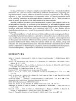
of orthophosphate traces. Two SIA methods using spectrophotometric detection, the
first based on the formation of an ionic association between molybdovanadophos-
phoric acid and the green malachite dye (Mu˜noz et al., 1997) and the second, in the
electrogeneration in the tubular flow electrodes of molybdenum blue (Mas et al.,
2004) (Figure 3.4.3), have been proposed for orthophosphate determination in these
Sample
SELECTION VALVE
BURETTE
Molybdate
Waste
Counter
electrode
HP-8452A
Working
electrode
Water
Air
NaOH
Ag/AgCI
SPECTROPHOTOMETER
POTENTIOSTAT
MAGNETIC
SITRRER
Figure 3.4.3 Schematic illustration of the sequential injection set-up devised for the spectropho-

tometric determination oforthophosphate based on theelectrochemical generation of molybdenum
blue
JWBK117-3.4 JWBK117-Quevauviller October 10, 2006 20:30 Char Count= 0
Chromatographic Methods 239
matrixes. Although the implementation of these new flow analysis methods has rep-
resented an important step forward in the application and automation of orthophos-
phate analysis methods, undoubtedly, the most interesting aspect is the possibility of
also carrying out the required on-line pretreatments, following methodologies with
high degrees of automation, which facilitate the determination of parameters such
as dissolved organic phosphorus (DOP) or dissolved total phosphorus (DTP). Thus,
FIA methods have been proposed with spectrophotometric detection, which use the
molybdenum blue formation reaction allowing the determination of DOP (Higuchi
et al., 1998) and DTP (Williams et al., 1993; Halliwell et al., 1996) in wastewaters. In
the former case the photo-oxidative and the acid hydrolysis methods are carried out
on-line. In this context it is worthwhile mentioning the FIA method (Benson et al.,
1996) which enables determination of total phosphorus (TP) and implies the use of
a combined photo-oxidation and thermal digestion system with which conversion of
condensed and organic phosphates into orthophosphates is carried out in the soluble
and particulate phase. Also, flow injection gel filtration techniques have been used
for speciation ofphosphorus compounds in wastewaters (McKelvie et al., 1993).FIA
methods (Miyazaki and Bansho, 1989; Manzoori et al., 1990) which use combined
spectrophotometry and inductively coupled plasma spectroscopy with optical detec-
tion techniques (FIA-ICP-AES) have been proposed to carry out rapid differential
determination of orthophosphate and total phosphate in wastewaters. As regards to
electric techniques, the following should be outlined: a FIA-potentiometric method
(De Marco et al., 1998), which uses a second-species cobalt wire ISE relied upon
cobalt phosphate determination for orthophosphate precipitation in wastewaters and
a FIA-amperometric method for the determination of total phosphorus in domestic
wastewaters, which uses continuous microwave oven decomposition with subse-
quent detection of orthophosphate (Hinkamp and Schwedt, 1990). In Table 3.4.2

are summarised the analytical characteristics of several of the above-mentioned
methods.
3.4.6 CHROMATOGRAPHIC METHODS
Analysis of nutrients in their inorganic form can be carried out in a simultaneous,
efficient and rapid way by application of a chromatographic method. Undoubtedly,
methods based on ion chromatography (IC) in its modality of ionic exchange with
eluent conductivity suppression, suppressed ion chromatography (SIC), have been
and currently are the most widely used since their introduction (Small et al., 1975).
On the other hand, it should be mentioned that this method became a standard method
for determination of chloride, bromide, nitrite, nitrate, phosphate and sulfate in
water and wastewaters. In wastewater analysis the only pretreatment of the sample
consists in its filtration through 0.45 μm membranes and NO
−
3
,NO
−
2
and PO
3−
4
contents are determined by SIC, and NH
+
4
content by automated wet chemistry, e.g.
FIA, SIA, etc. In this context Matsui et al. (Matsui et al., 1997) have proposed a
method for the determination of ammonium, nitrite, nitrate, chloride and sulfate
in wastewaters. Ammonium is spectrophotometrically detected in a FIA system by
JWBK117-3.4 JWBK117-Quevauviller October 10, 2006 20:30 Char Count= 0
Table 3.4.2 Analytical characteristics of some flow analysis methods for orthophosphate determination in wastewaters
Flow Detection Detection limit Sampling

system technique Reagents Linear range (mg P/l) RSD% (mg P/l) (mg P/l) rate (/h) Reference
FIA Spec Mo-V Up to 200 2 (10) 0.8 8 Manzoori et al., 1990
FIA Spec Mo/Sn-Hy 0–25 0.4 (8,75) 0.05 20 Benson et al., 1996a,b
FIA Spec Mo-Sb/Asc 0.001–0.05 1.0 (0.020) 0.0006 12 Korenaga and Sun,
1996
FIA Spec DR: Perox + H2SO4,
Mo-Sb/Asc-NaDS
0.10–1.0 2.25–0.13(0.024–3.03) 0.001 20 Higuchi et al., 1998
FIA Spec MWD in HNO
3
medium, Mo/Asc
Up to 6.53 <5.0 (0.033–6.53) 0.033 30 Williams et al., 1993
FIA Spec DR: Perox + HClO4,
Mo/Sn-Hy
0–18 ≤2.0 (10.2) 0.15 32 Benson et al., 1996a,b
IC-FIA Spec TD in H
2
SO
4
medium,
Mo/Sn-Hy
Or: 0.010–1.00 Pyr
and Tri: 0.020–2.00
≤3.0 (1.00) Or: <0.01 Pyr and
Tri: 0.020
5 Halliwell et al., 1996
SIA Spec Mo-V Up to 18.00 2.1(5.00) 0.15 30 Mu˜noz et al., 1997
SIA Spec Mo-V-MG 0.05–0.40 18(0.10) 0.01 30 Mu˜noz et al., 1997
SIA Spec Mo/Sn 0.05–4.00 1.7(2.50) 0.01 30 Mu˜noz et al., 1997
SIA Spec Mo/SSTFTE 0.3–20 1.8(10) 0.1 18 Mas et al., 2004

SIA Spec Mo-V Up to 12 1.4 (9) 0.2 23 Mas et al., 1997
SIA Spec Mo-V 0.8–15 2.1(5.0) 0.23 30 Mas et al., 2000
MCFIA Spec Mo-Sb/Asc Up to 3 1.4(2.47) NR 180 Wang et al., 1998
FIA Spec +
ICP-AES
Spec: Mo-V Up to 200 Or and TP ICP: 2.01 (10) Spec: 0.8 ICP:0.5 80 Manzoori et al., 1990
FIA Pot Pht-CoW 3.1–310 4.0 (31) 0.093 NR De Marco et al., 1998
FIA Amp MWD/DR: Perox or
HClO
4
Up to 30 3 (5.0) 0.10 21 Hinkamp and Schwedt,
1990
RSD, relative standard deviation; NR, not reported Detection technique: Spec (spectrophotometric), ICP (inductively coupled plasma), AES (atomic emission spectrophotometry),
Pot (potentiometric), Amp (amperometric). Reagents: Mo (potassium ammonium molybdate), V (ammonium vanadate), Sn [tin (II)], Hy (hydrazine), Sb (antimony tartrate), Asc
(ascorbic acid), DR (digestion reagent), Perox ( sodium peroxydisulfate), NaDS (sodium dodecylsulfate), MWD (microwave digestion), TD (thermal digestion), MG (malachuite
green), SSTFTE (stainless steel tubular flow-through electrode), Pht (phthalate buffer), CoW (cobalt wire electrode), Or (orthophosphate), Pyr (pyrophosphate), Tri (triphosphate),
TP (total phosphorus).
240
JWBK117-3.4 JWBK117-Quevauviller October 10, 2006 20:30 Char Count= 0
References 241
a postcolumn derivatization reaction using the indophenol reaction, and the other
ions by conductimetric detection. In other studies (Karmarkar, 1998, 1999) the use
of this strategy is also proposed for nutrient analysis in wastewaters. In Karmarkar’s
first study (Karmarkar, 1999) a sequential IC-FIA method is used which allows de-
termination in only one injection of NO
−
3
,PO
3−
4

and NH
+
4
. Ammonium is determined
at the outlet of the column in the void volume by a FIA system and the remaining
analytes with a conductimetric detector in the usual SIC way. In Karmarkar’s second
study (Karmarkar, 1998) F
−
,Cl
−
,NO
−
3
,Br
−
, HPO
2−
4
and SO
2−
4
are analysed in
wastewaters by enhanced IC with sequential FIA. The use of on-line dialysis has
been proposed for automation of sampling and pretreatment of wastewater samples
in order to carry out the analysis of ions and small molecules by FIA and chromatog-
raphy,in a fast economical way and without analyte loss (Frenzel, 1997). Laubli et al.
(Laubli et al., 1999) have determined F
−
,Cl
−

,NO
−
2
,NO
−
3
,Br
−
,PO
3−
4
and SO
2−
4
in wastewaters by SIC using a Metrosep Anion Dual 2 column, and a mixture of
NaHCO
3
and Na
2
CO
3
as eluent, in combination with a sample pretreatment in an
on-line dialysis unit and using a stop-flow technique.
3.4.7 CAPILLARY ELECTROPHORESIS METHODS
This technique presents sensitivity, low sample consumption, high resolution and it
is fast in relation to chromatographic methods. However, there are few literature data
with regard to the application of this technique to nutrient analysis in wastewaters.
One of the few applications, which can illustrate the potential of this technique, is
that described by Pantsar-Kallio et al. (Pantsar-Kalio et al., 1997). These authors
propose a method which allows separating and determining a total of nine organic

acids and seven inorganic anions (Cl
−
,SO
2−
4
,NO
−
2
,NO
−
3
,F
−
,PO
3−
4
and CO
2−
3
)in
wastewaters. The method uses pyridine-2,6-dicarboxylic acid as electrolyte, tetrade-
cyltrimethylammonium bromide as electro-osmotic flow modifier and the analytes
were detected by measuring indirect UV absorption.
REFERENCES
Alexander, P.W., Dimitrakopoulos, T. and Hibbert D.B. (1997) Electroanalysis, 9(17), 1331–
1336.
Alexander, P.W., Dimitrakopoulos, T. and Hibbert, D.B. (1998) Electroanalysis, 10(10), 707–712.
Alexander, P.W., Di Benedetto, L.T., Dimitrakopoulos, T., Hibbert, D.B., Ngila, J.C., Sequeira, M.
and Shiels, D. (1996) Talanta, 43(6), 915–925.
Andrew, K.,. Worsfold, P.J. and Comber, M. (1995) Anal. Chim. Acta, 314(1–2), 33–43.

Aoki, T. and Wakabayashi, M. (1995) Anal. Chim. Acta, 308 (1–3), 308–312.
Aoki, T., Fukuda, S., Hosoi, Y. and Mukai, H. (1997) Anal. Chim. Acta, 349(1–3), 11–16.
Aoyagi, M., Yasumasa, Y. and Nishida, A. (1989) Anal. Sci., 5 (2), 235–236.
Akse, J.R., Thompson, J.O., Sauer, R.L. and Atwater, J.E. (1998) Microchem. J., 59(3), 372–382.
JWBK117-3.4 JWBK117-Quevauviller October 10, 2006 20:30 Char Count= 0
242 Nutrient Control
American Public Health Association-American Water Works Association-Water Pollution Control
Federation (APHA-AWWA-WPCF). (2000) Standard Methods for the Examination of Water
and Wastewater, 20th ed. APHA, Washington, DC.
APHA Method 4110 B. (2000) Chromatographic Method.
APHA Method 4500-N B. (2000) In-line UV/Persulfate Digestion and Oxidation with Flow In-
jection Analysis.
APHA Method 4500-N C. (2000) Persulfate Method.
APHA Method 4500-NH
3
B (2000) Preliminary Distillation Step.
APHA Method 4500-NH
3
C. (1992) Nesslerization method. StandardMethods forthe Examination
of Water and Wastewater, 17th ed. American Public Health Association-American Water Works
Association-Water Pollution Control Federation (APHA-AWWA-WPCF).APHA,Washington,
DC.
APHA Method 4500-NH
3
C. (2000) Titrimetic Method.
APHA Method 4500-NH
3
D. (2000) Ammonia Selective Electrode Method.
APHA Method 4500-NH
3

E. (2000) Ammonia Selective Electrode Method Using Known Addi-
tion.
APHA Method 4500-NH
3
F. (2000) Phenate Method.
APHA Method 4500-NH
3
G. (2000) Automated Phenate Method.
APHA Method 4500-NH
3
H. (2000) Flow Injection Analysis.
APHA Method 4500-NO
−
2
B. (2000) Colorimetric Method.
APHA Method 4500-NO
−
3
D. (2000) Nitrate Electrode Method.
APHA Method 4500-NO
−
3
E. (2000) Cadmium Reduction Method.
APHA Method 4500-NO
−
3
F. (2000) Automated Cadmium Reduction Method.
APHA Method 4500-NO
−
3

G. (1992) Method of reduction with titanuos chloride. Standard
Methods for the Examination of Water and Wastewater, 17th ed. American Public Health
Association-American Water Works Association-Water Pollution Control Federation (APHA-
AWWA-WPCF). APHA, Washington, DC.
APHA Method 4500-NO
−
3
H. (2000) Automated Hydrazine Reduction Method.
APHA Method 4500-NO
−
3
I. (2000) Cadmium Reduction Flow Injection Method.
APHA Method 4500-N
org
. (2000) Nitrogen Organic Method.
APHA Method 4500-N
org
B. (2000) Macro-Kjeldhal Method.
APHA Method 4500-N
org
C. (2000) Semi-Micro Kjeldhal Method.
APHA Method 4500-N
org
D. (2000) Block Digestion and Flow Injection Analysis.
APHA Method 4500-P B. (2000) Sample Preparation.
APHA Method 4500-P C. (2000) Vanadomolybdophophoric Acid Colorimetric Method.
APHA Method 4500-P D. (2000) Stannous Chloride Method.
APHA Method 4500-P E. (2000) Ascorbic Acid Method.
APHA Method 4500-P F. (2000) Automated Ascorbic Acid Reduction Method.
APHA Method 4500-P G. (2000) Flow Injection Analysis for Orthophosphate.

APHA Method 4500-P H. (2000) Manual Digestion and Flow Injection Analysis for Total Phos-
phorus.
APHA Method 4500-P I. (2000) In-line UV/Persulfate Digestion and Flow Injection Analyis for
Phosphorus.
Armstrong, D.E. (1972) In: M. Halmann (Ed.), Analytical Chemistry of Phosphorus Compounds.
Wiley/Interscience, New York, pp. 744–769.
Benson, R.L., McKelvie, I.D., Hart, B.T., Truong, Y.B. and Hamilton, I.C. (1996a) Anal. Chim.
Acta, 326(1–3), 29–39.
Benson, R.L., Truong, Y.B., McKelvie, I.D. and Hart, B.T., (1996b) Water Res., 30(9), 1959–1964.
Brober, O. and Persson, G. (1988) Hydrobiologia, 170, 61.
JWBK117-3.4 JWBK117-Quevauviller October 10, 2006 20:30 Char Count= 0
References 243
Burden, E.H.W.J. (1961) Analyst 86, 429–433.
Carrer, I., Cusmai, P., Zanzottera, E., Martinotti, W. and Realini, F. (1995) Anal. Chim. Acta, 308
(1–3), 20–27.
Catala-Icardo, M., Martinez-Calatayud, J. and Garcia-Mateo, J.V. (2001) Analyst, 126(8), 1423–
1427.
Cerd`a, A, Oms, M.T. and Cerd`a, V. (2000) Determination of Organic Nitrogen: Handbook of Water
Analysis. Marcel Dekker Inc., New York.
Cerd`a, A., Oms, M.T., Cerd`a, V. and Forteza, R. (1995) Anal. Methods Instrum., 2(6), 330–336.
Cerd`a, A., Oms, M.T., Forteza, R. and Cerd`a, V. (1996) Analyst, 121(1), 13–17.
Cerd`a, A., Oms, M.T., Forteza, R. and Cerd`a, V. (1997) Anal. Chim. Acta, 351(1–3), 273–279.
Clementson, L.A. and Wayte, S.E. (1992) Water Res., 26(9), 1171–1176.
Cliford, D.A. and McGaughey, L.M. (1982) Anal. Chem., 54(8), 1345–1350.
Colin, F. and Quevauviller, P. (Eds) (1998) Monitoring of Water Qualitity, Proceedings of the
European Workshop on Standards, Measurements and Testing. Elsevier, Amsterdam.
Cosano, J.S., Luque de Castro, M.D. and Valc´arcel, M. (1993) J. Autom. Chem., 15(4), 147–150.
Daughton, C.G., Jones, B.M. and Sakaji, R.H. (1985) Anal. Chem., 57(12), 2326–2333.
Davidson, J., Mathieson, J. and Boyne, A.W. (1970) Analyst, 95(127), 181–193.
De Marco, R., Pejcic, B. and Chen, Z.L. (1998) Analyst, 123(7), 1635–1640.

Dimitrakopoulos, T., Alexander, P.W. and Hibbert. D.B. (1996) Electroanalysis, 8(5), 438–442.
Dore, J.E., Houlihan, T.,. Hebel, D.V, Tien, G., Tupas, L. and Karl, D. M. (1996) Mar. Chem.,
53(3/4), 173–185.
Ebina, J., Tsutsui, T. and Shirai, T. (1983) Water Res., 17(12), 1721–1726.
Forman, D., Al-Dabbaghand, S. and Doll, R. (1985) Nature, 313 (6004), 620–625.
Frenzel, W. (1997) GIT Labor-Fachzeitschrift, 41(7), 734, 736–738, 740–741.
Frenzel, W., Schulz-Brussel, J. and Zinvirt, B. (2004) Talanta, 64(2), 278–282.
Gabriel, D., Baeza, J., Valero, F. and Lafuente, J. (1998) Anal. Chim. Acta, 359(1–2), 173–183.
Galhardo, C.X. and Masini, J.C. (2001) Anal. Chim. Acta, 438(1–2), 39–48.
Gil-Torro, I., Garc´ıa-Mateo, J.V. and Mart´ınez-Calatayud, J. (1998) Anal. Chim. Acta, 366(1–3),
241–249.
Halliwell, D.J., McKelvie, I.D., Hart, B.T. and Dunhill, R.H. (1996) Analyst, 121(8), 1089–1093.
Hanrahan, G., Ussher, S., Gledhill, M., Achterberg, E.P. and Worsfold, P.J. (2002) Trends Anal.
Chem., 21(4), 233–239.
Higuchi, K., Tamanouchi, H. and Motomizu, S. (1998) Anal. Sci., 14(5), 941–946.
Hinkamp, S. and Schwedt, G. (1990) Anal. Chim. Acta, 236(2), 345–350.
Hirakawa, K. Yoshida, I. and Ishii, D. (1998) Bunseki Kagaku, 47(6), 341–348.
Johnson, C.J. and Cross, B.C. (1990) Am. J. Ind. Med., 18(4), 449–456.
Karmarkar, S.V. (1998) Am. Environ. Lab., 10
(2), 6–7.
Karmarkar, S.V. (1999) J. Chromatogr. A, 850(1 and 2), 303–309.
Korenaga, T. and Sun, F.S. (1996) Talanta, 43(9), 1471–1479.
Koroleff, F. (1969) Determination of total nitrogen in natural waters by means of persulfate oxi-
dation. Congress for Exploration of the Sea (ICES), Poster C8.
Kurzawa, C., Schuhmann, W., Wang, L., Orth, H., Schwendtke, I., Gerberding, H., Stadler, H. and
Grundig, B. (2001) GIT Labor-Fachzeitschrift, 45(2), 156–160.
Kuznetsov, V.V., Zemyatova, S.V. and Ermolenko, Y.V. (2005) J. Anal. Chem., 60(3), 289–296.
Lapa, R.A.S., Lima, J.L.F.C. and Pinto, I.V.O.S. (2000) Analusis, 28(4), 295–301.
Laubli, M., Sugai, T., Ono, J. and Schafer, H. (1999) Kogyo Yosui, 493, 32–34.
Manzoori, J.L., Miyazaki, A. and Tao, H. (1990) Analyst, 115(8), 1055–1058.

Mas, F., Estela, J.M., Miro, M., Cladera, A. and Cerda, V. (2004) Anal. Chim. Acta, 510(1), 61–68.
Mas, F., Mu˜noz, A., Estela, J.M. and Cerd`a, V. (1997) Analyst, 122(10), 1033–1038.
JWBK117-3.4 JWBK117-Quevauviller October 10, 2006 20:30 Char Count= 0
244 Nutrient Control
Mas, F., Mu˜noz, A., Estela, J.M. and Cerd`a, V. (2000) Int. J. Environ. Anal. Chem., 77(3), 185–202.
Matsui, M., Gotoh, T., Ishibashi, T. and Nishikawa, M. (1997) Kankyo Kagaku, 7(1), 23–30.
McKelvie, I.D. (2000) Phosphates: Handbook of Water Analysis. Marcel Dekker, Inc., New York.
McKelvie, I.D., Peat, D. and Worsfold, P.J. (1995) Anal. Proc., 32 (10), 437–445.
McKelvie, I.D., Hart, B.T., Cardwell, T.J. and Cattrall, R.W. (1993) Talanta, 40(12), 1981–1993.
Menezes-Santos, M., Reis, B.F., Bergamin, H. and Baccan, N. (1992) Anal. Chim. Acta, 261(1–2),
339–343.
Miura, Y. and Kusakari, K. (1999) Anal. Sci., 15( 9), 923–926.
Miyazaki, A. and Bansho, K. (1989) Kogai, 24(2), 87–93.
Mopper, K. and Zika, R.G. (1987) Nature, 325(6110), 246–249.
Moschou, E., Chaniotakis, N. A., Papandroulakis, N. and Divanach, P. (1998) Am. Environ. Lab.,
10(7), 10–12.
Mulvaney, R.L., Strle, K. and Horgan, B.P. (2000) J. Environ. Qual., 29(6), 1890–1895.
Mu˜noz, A., Mas, F., Estela, J.M. and Cerd`a, V. (1997) Anal. Chim. Acta, 350(1–2), 21–29.
Muraki, H., Higuchi, K., Sasaki, M., Korenaga, T. and Toei, K. (1992) Anal. Chim. Acta, 261(1–2),
345–349.
Nakata, R., Terashita, M., Nitta, A. and Ishikawa, K. (1990) Analyst, 115(4), 425–430.
Nidal, F. (1978) Water Res., 12(12), 1123–1130.
Nikonorov, V.V. and Moskvin, L.N. (1995) Anal.Chim Acta, 306(2–3), 357–360.
Nobrega, J.A., Mozeto, A.A., Alberici, R.M. and Guimaraes, J.L. (1995) J. Braz. Chem. Soc., 6(4),
327–330.
Nollet, L.M.L. (ED.) (2000) Handbook of Water Analysis. Marcel Dekker, Inc., New York.
Oleksy-Frenzel, J. and Jekel, M. (1996) Anal.Chim. Acta, 319(1–2), 165–175.
Oms, M.T., Cerd`a, A. and Cerd`a, V. (1995) Anal. Chim. Acta, 315(3), 321–330.
Oms, M.T., Cerd`a, A. and Cerd`a, V. (1996) Electroanalysis, 8(4), 387–390.
Pantsar-Kallio, M., Kuitunen, M. and Pentti, P.K.G. (1997) Chemosphere, 35(7), 1509–1518.

Robards, K., McKelvie, I.D., Benson, R.L., Worsfold, P.J., Blundell, N. and Casey H. (1994) Anal.
Chim. Acta, 287(3), 147–190.
Russell. S. (1994) Ammonia. WRc Instrument Handbooks, Swindon, UK.
Segarra-Guerrero, R., Gomez-Benito, C. and Martinez-Calatayud, J. (1996) Talanta, 43(2), 239–
246.
Shen, H., Cardwell, T.J. and Cattrall, R.W. (1997) Analyst, 122(1), 89–93.
Shen, H., Cardwell, T.J. and Cattrall, R.W. (1998) Anal. Chim. Acta, 367(1–3), 193–199.
Small, H., Stevens, T.S. and Bauman, W.C. (1975) Anal. Chem., 47(11), 1801–1809.
Standard Methods Committee. (1988) American Public Health Association-American Water
Works Association-Water Pollution Control Federation (APHA-AWWA-WPCF).
Standards Australia and Standards New Zealand. (1998) Australian/New Zealand, Water Quality-
Sampling. Part 1: Guidance on the Design of Sampling Programs, Sampling Techniques and
the Preservation and Handling of Samples.
Stumm, W. and Morgan, J.J. (1996) Aquatic Chemistry, 3rd ed. Wiley, New York.
Su, X.L., Chen, P., Qu, X.G., Wei, W.Z. and Yao, S.Z. (1998) Microchem. J., 59(3), 341–350.
Thomas, O., Theraulaz, F., Cerd`a, V., Constant, D. and Quevauviller, Ph. (1997) Trends Anal.
Chem., 16(7), 419–424.
Trojanowicz, M., Benson, R.L. and Worsfold, P.J. (1991) Trends Anal. Chem.,
10(1), 11–17.
Van Staden, J.F. and van der Merwe, T.A. (1998) Mikrochim. Acta, 129(1–2), 33–39.
Vlcek, J. and Kuban, V. (1999) Coll. Czech. Chem. Commun., 64(12), 1966–1974.
Wang, J. and He, R. (1995) Huanjing Kexue, 16(1), 71–73.
Wang, L., Cardwell, T.J., Cattrall, R.W., Luque de Castro, M.D. and Kolev, S.D. (2000) Anal. Chim.
Acta, 416(2), 177–184.
JWBK117-3.4 JWBK117-Quevauviller October 10, 2006 20:30 Char Count= 0
References 245
Wang, X.D., Cardwell, T.J., Cattrall, R.W., Dyson, R.P. and Jenkins, G.E. (1998) Anal. Chim. Acta,
368(1–2), 105–111.
Williams, K.E., Haswell, S.J., Barclay, D.A. and Preston, G. (1993) Analyst, 118(3), 245–248.
Zi, Y. and Chen, L. (2000a) Fenxi Ceshi Xuebao, 19(2), 70–72.

Zi, Y. and Chen, L. (2000b) Fenxi Huaxue, 28(3), 395.
Zi, Y., Duan, L. and Lu, Ch. (2001) Fenxi Huaxue, 29(2), 186–188.
JWBK117-4.1 JWBK117-Quevauviller October 10, 2006 20:31 Char Count= 0
4.1
State Estimation for Wastewater
Treatment Processes
Olivier Bernard, Benoˆıt Chachuat, and Jean-Philippe Steyer
4.1.1 Introduction
4.1.2 Preliminaries
4.1.2.1 Notion of Observability
4.1.2.2 General Definition of an Observer
4.1.3 Observers for Linear Systems
4.1.3.1 Luenberger Observer
4.1.3.2 The Linear Case up to an Output Injection
4.1.3.3 Kalman Filter
4.1.3.4 The Extended Kalman Filter
4.1.3.5 Application to an Alternating-activated-sludge Plant
4.1.4 Observers for Mass-balance-based Systems
4.1.4.1 Preliminaries
4.1.4.2 Asymptotic Observers
4.1.4.3 Application to an Anaerobic Digester
4.1.5 Interval Observers
4.1.5.1 Principle
4.1.5.2 Application to an Anaerobic Digester
4.1.6 Conclusions
References
Wastewater Quality Monitoring and Treatment Edited by P. Quevauviller, O. Thomas and A. van der Beken
C

2006 John Wiley & Sons, Ltd. ISBN: 0-471-49929-3

JWBK117-4.1 JWBK117-Quevauviller October 10, 2006 20:31 Char Count= 0
248 State Estimation for Wastewater Treatment Processes
4.1.1 INTRODUCTION
A major bottleneck in the application of advanced monitoring and optimization
strategies for wastewater treatment plants (WWTPs) lies in the difficulty of measur-
ing chemical and biological variables. Even though considerable progress in on-line
sensor technology has been made over recent years, it is still often difficult to mea-
sure many of the key state variables such as biomass concentration, specific bacte-
rial activity or intermediate product concentration. Hence, the idea arose of using
observers, also called software sensors, that combine a number of readily available
on-line measurements (gaseous flow rates, pH, dissolved gases, etc.) with a process
model for estimating the values of (unmeasured) state variables.
Quite a few methods have been proposed to design such observers. In this chapter,
we shall only focus on those approaches that are relevant to the field of WWTPs.
It is worthwhile noting that the principles underlying the design of observers can
be quite different. Therefore, the choice of an observer inherently depends on the
specificities of the problem at hand. In practice, this choice is strongly guided by the
reliability of the process model as well as the amount and accuracy of the data. If a
reliable process model is available and if this model has been thoroughly identified
and validated, either an (extended) Kalman filter or a high gain observer can be
developed. When the process model is not accurate enough, an asymptotic observer
relying on mass-balance principles, but not on the uncertain kinetics, shall be used
instead. Finally, if bounds are known for the uncertain inputs and/or parameters,
an interval observer can be used for predicting intervals in which the unmeasured
variable are guaranteed to belong (instead of point-wise estimates).
The type of observer to be constructed should not only be based on the model
quality, but it must also account for the objectives to be achieved. Indeed, an observer
can have other purposes than simply monitoring a WWTP. It can be developed with
the objective of applying a control action that needs an estimate of some internal
state; it can also be used for diagnosing whether a failure occurred during process

operation or not.
The remainder of this chapter is organized as follows. A number of useful def-
initions and results are given in Section 4.1.2. Observers that require a full-model
description of the process are presented in Section 4.1.3, with emphasis placed on
linear systems. The design of observers relying on the mass-balance principles is
discussed in Section 4.1.4. Interval observers that exploit knowledge of bounds on
the model uncertainty are presented in Section 4.1.5. Finally, Section 4.1.6 concludes
the chapter.
4.1.2 PRELIMINARIES
This section gives an overview of the main theoretical concepts in system observabil-
ity. These concepts are usefulin the analysis conducted later on. Theinterested reader
JWBK117-4.1 JWBK117-Quevauviller October 10, 2006 20:31 Char Count= 0
Preliminaries 249
is referred to Luenberger (Luenberger, 1979) and Gauthier and Kupka (Gauthier and
Kupka, 2001) for additional information.
It is first fundamental to study the observability property of a system prior to
designing an observer. Intuitively, observability consists of determining whether the
measured signals contain sufficiently rich information to estimate the unmeasured
state variables; a system is then said to be observable if it satisfies this property from
a theoretical point of view. The problem to address next is to derive an observer
for the problem at hand, i.e. an auxiliary dynamic system that provides the state
estimates. At this point, it should be noted that the problems of observability and
observer design are very different in nature. In particular, the observability property
does not give any clue on how to build an observer.
The theory of observation has been extensively developed in the linear case.
Several methods also exist in the nonlinear case, but are tailored to specific classes
of models.
4.1.2.1 Notion of Observability
We consider the following general model driving the process dynamics:
⎧

⎨
⎩
dx(t)
dt
= f
[
x(t), u(t)
]
; x(0) = x
0
y(t) = h[x(t)]
(S )
where u ∈ 
m
is the input vector, y ∈ 
p
is the output vector and x ∈ 
n
is the state
vector made up of the concentrations of the various species inside the liquid phase;
x
0
is the vector of initial conditions. The applications f and h provide the dynamics
of the state variables and the links between the state variables and the measurements,
respectively.
The objective is to estimate x(t) from the measurements y(t). Observability is a
structural property of a system that states whether this is possible or not.
Property 1. The system (S ) is said to be observable, if x(t) can be uniquely deter-
mined from
y(t),

dy(t)
dt
,
d
2
y(t)
dt
2
, ,
d
n
y
y(t)
dt
n
y
and
u(t),
du(t)
dt
,
d
2
u(t)
dt
2
, ,
d
n
u

u(t)
dt
n
u
for some (possibly infinite) n
y
≥ 0 and n
u
≥ 0.
JWBK117-4.1 JWBK117-Quevauviller October 10, 2006 20:31 Char Count= 0
250 State Estimation for Wastewater Treatment Processes
u
y
Process
x
x
Observer
z
Figure 4.1.1 Observer principle
The reader is referred to Luenberger (Luenberger, 1979) and Gauthier and Kupka
(Gauthier and Kupka, 2001) for more details.
4.1.2.2 General Definition of an Observer
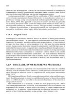
Once a system has been shown to be observable, the next step is to design an
observer that estimates the state variable x based on a model and a set of input/output
measurements. The principle of an observer is presented in Figure 4.1.1. Roughly
speaking, an observer is an auxiliary dynamic system coupled to the original system
via the measured inputs and outputs. This is formalized in the following definition.
Definition 1. An observer is an auxiliary system (O) coupled to the original system
(S) as:
⎧

⎨
⎩
dz(t)
dt
=
ˆ
f
[
z(t), u(t), y(t)
]
; z(0) = z
0
ˆ
x(t) =
ˆ
h
[
z(t), u(t), y(t)
]
(O)
where z ∈ 
q
denotes the state of the observer,
ˆ
f is the observer dynamics and
ˆ
h
relates z to the estimate
ˆ
x of the real system. An observer has the property that the

observation error converges to zero asymptotically:
lim
t→∞

ˆ
x(t) − x(t)

= 0
A desirable property for an observer is the ability to tune the convergence rate in
order for the estimates to converge more rapidly than the original dynamics of the
system. Another desirable property is that the estimate
ˆ
x(t) should remain equal to
x(t) under proper initialization, i.e. when it is initialized with the true value x(0).
This easily justifies that the following structure is often used to design observers in
practice:
⎧
⎪
⎪
⎨
⎪
⎪
⎩
d
ˆ
x(t)
dt
= f
[
ˆ

x(t), u(t)
]
+ k
{
z(t), [h
[
ˆ
x(t) − y(t)
]
]
}
dz(t)
dt
=
ˆ
f
[
z(t), u(t), y(t)
]
with k
[
z(t), 0
]
= 0
JWBK117-4.1 JWBK117-Quevauviller October 10, 2006 20:31 Char Count= 0
Observers for Linear System 251
This observer consists of a replica of the original dynamics corrected by a term that
depends on the discrepancy between both the measured and predicted outputs. Note
also that the correction amplitude is tuned via the function k that is often referred to
as the observer gain (internal tuning of the observer).

4.1.3 OBSERVERS FOR LINEAR SYSTEMS
For time-invariant, linear systems, the general system (S) simplifies to:
⎧
⎨
⎩
dx(t)
dt
= Ax(t) + Bu(t)
y(t) = Cx(t)
(S
L
)
with A ∈ 
n×n
(n ≥ 2) and C ∈ 
p×n
. A well-known observability criterion for
(S
L
) is given by the rank condition:
rank
⎛
⎜
⎜
⎜
⎝
C
CA
.
.

.
CA
n−1
⎞
⎟
⎟
⎟
⎠
= n
4.1.3.1 Luenberger Observer
Theorem 1. If thepair (A,C) isobservable, a Luenberger observer for (S
L
) is obtained
as (Luenberger, 1966):
d
ˆ
x(t)
dt
= A
ˆ
x(t) + Bu(t) + K
[
C
ˆ
x(t) − y(t)
]
(O
L
)
where K is a n × n gain matrix that can be used for tuning the convergence rate of

the observer, and can be chosen in order for the observation error to converge to zero
arbitrarily fast.
Proof. The dynamics of the observation error e(t) =
ˆ
x(t) − x(t)isgivenby:
de
dt
= (A +KC )e
and is independent of the input u(t). The result follows from the pole placement
theorem which guarantees that the error dynamics can be chosen arbitrarily.
In principle, the gain matrix K can be chosen in such a way that the observation
error converges to zero as quickly as desired. However, the larger the gain of the
JWBK117-4.1 JWBK117-Quevauviller October 10, 2006 20:31 Char Count= 0
252 State Estimation for Wastewater Treatment Processes
observer, the more sensitive it becomes toexternal perturbations (measurement noise
for example). A good compromise must thus be sought that ensures both stability
and accuracy at the same time. The Kalman filter, discussed in the subsection below,
proposes a way of achieving such a compromise.
4.1.3.2 The Linear Case up to an Output Injection
A particular situation wherein a linear observer can be designed for a nonlinear
system arises in the simple case where the nonlinearities depend on the output y
only:
⎧
⎨
⎩
dx(t)
dt
= Ax(t) +φ
[
t, y(t)

]
+ Bu(t)
y(t) = Cx(t)
with φ being a (known) nonlinear function in 
n
. The following ‘Luenberger-like’
observer has linear dynamics with respect to the observation error:
d
ˆ
x(t)
dt
= A
ˆ
x(t) +φ
[
t, y
(
t
)
]
+ Bu(t) + K
[
C
ˆ
x(t) − y(t)
]
In particular, the error dynamics can be chosen arbitrarily, provided that the pair
(A,C) is observable. Here again, however, an adequate choice for the gain vector K
is one that guarantees a fast enough convergence of the observer, while keeping it
stable.

4.1.3.3 Kalman Filter
The Kalman filter is notorious in the field of linear systems (Lewis, 1986). Loosely
speaking, a Kalman filter can be seen as a Luenberger observer with a time varying
gain. More specifically, the gain is chosen in such a way that the variance of the
observation error is minimized (or, equivalently, the integral between t
0
and t of the
squared errors is minimized); for this reason the Kalman filter is often referred to as
the optimal estimator.
Consider an observable continuous-time system in the following stochastic rep-
resentation:
dx(t)
dt
= Ax(t) + Bu(t) + Gω(t); x(t
0
) = x
0
(1)
where ω ∼ [0, Q(t)] is a white noise process with zero mean and covariance Q(t).
Suppose that initial state x
0
is unknown, but there is available a priori knowledge
JWBK117-4.1 JWBK117-Quevauviller October 10, 2006 20:31 Char Count= 0
Observers for Linear System 253
that x
0
∼ (
¯
x
0

, P
0
). Suppose also that measurements are given at discrete times t
k
according to:
y
k
= Cx(t
k
) + v
k
(2)
where v
k
∼ (0, R
k
) is uncorrelated with ω(t) and x
0
.
Besides initialization, acontinuous/discrete Kalman filterfor system(1,2) consists
of two steps: a propagation step (between two successive measurements), followed
by a correction step (at measurement times):
Initialization (t = t
+
0
)
P
(
t
0

)
= P
0
,
ˆ
x(t
0
) =
¯
x
0
Propagation (t
+
k−1
≤ t ≤ t
−
k
, k ≥ 1)
⎧
⎪
⎪
⎨
⎪
⎪
⎩
dP(t)
dt
= AP(t) + P(t)A
T
+ GQ(t)G

d
ˆ
x(t)
dt
= A
ˆ
x(t) + Bu(t)
Correction (t = t
+
k
, k ≥ 1)
⎧
⎪
⎪
⎨
⎪
⎪
⎩
K
k
= P(t
−
k
)C
T

CP (t
−
k
)C

T
+ R
k

−1
P(t
+
k
) =
[
I − K
k
]
P(t
−
k
)
ˆ
x(t
+
k
) =
ˆ
x(t
−
k
) + K
k

z

k
−C
ˆ
x(t
−
k
)

At this point, we shall emphasize several points. Note first that the foregoing Kalman
filter can be applied to time-varying linear system, i.e. with matrices A, B, C and
G depending on time. One should however keep in mind that observability must be
proven for such systems prior to constructing the observer. Note also that Kalman
filters can be extended by adding a term −θP(t), θ>0, in the propagation equation
of P. This exponential forgetting factor allows us to consider the case where Q = 0.
Finally, estimating the positive definite matrices R, Q and P
0
often proves to be
tricky in practice, especially when the noise properties are not known precisely.
4.1.3.4 The Extended Kalman Filter
Consider a continuous-time nonlinear system of the form:
dx(t)
dt
= f
[
x(t), u(t)
]
+ Gω(t); x(t
0
) = x
0

(3)
JWBK117-4.1 JWBK117-Quevauviller October 10, 2006 20:31 Char Count= 0
254 State Estimation for Wastewater Treatment Processes
with measurements at discrete time t
k
given by:
y
k
= h[x(t
k
)] + v
k
(4)
The idea behind the Extended Kalman Filter (EKF) is to linearize the nonlinear
system (3,4) around its current state estimate
ˆ
x(t) (Lewis, 1986). By doing so, the
problem becomes equivalent to building a Kalman filter for a nonstationary linear
system (1,2) with A and C taken as:
A(t) =

∂ f
∂x

x(t)
C(t
k
) =

∂h

∂x

x(t
k
)
The EKF is used routinely and successfully in many practical applications, including
WWTPs, even though few theoretical guarantees can be given as regards its conver-
gence (Lewis, 1986; Bastin and Dochain, 1990). Note also that multirate versions
of the EKF have been developed to handle those (rather frequent) situations where
measurements are available at different samplings rates (Gudi et al., 1995). An ap-
plication of EKF in alternating activated sludge WWTPs is detailed hereafter. Other
applications to the activated sludge process can be found (Zhao and K¨ummel, 1995;
Lukasse et al., 1999).
4.1.3.5 Application to an Alternating-activated-sludge Plant
We consider an alternating-activated-sludge (AAS) WWTP similar to the one shown
in Figure 4.1.2. AAS plants degrade both organic and nitrogenous compounds by
alternating aerobic and anoxic phases in the bioreactor. Besides dissolved oxygen
(DO) concentration that is routinely measured in activated sludge WWTPs, both ni-
trate and ammonia concentrations can also be measured on-line (at a lower frequency
than DO, though). The objective here is to estimate the concentration of COD in the
bioreactor based on these measurements.
effluent
settler
aeration tank
recycled sludge wasted sludge
influent
Figure 4.1.2 Typical small-size alternating activated sludge treatment plant
JWBK117-4.1 JWBK117-Quevauviller October 10, 2006 20:31 Char Count= 0
Observers for Mass-balance-based System 255
80

100
120
140
160
180
200
220
240
(a)
(b)
9:00
11:00
13:00
15:00
17:00
19:00
21:00
COD (mg/l)
Time (hh:mm)
open-loop
EKF
true state
-120
-100
-80
-60
-40
-20
0
20

40
9:00
11:00
13:00
15:00
17:00
19:00
21:00
Error (mg/l)
Time (hh:mm)
EKF
open-loop
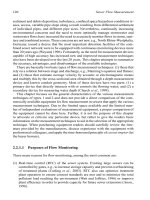
Figure 4.1.3 Estimated COD concentration (a) and observation error (b)
A multirate EKF is developed based on the reduced nonlinear model given in
Chachuat et al. (Chachuat et al., 2003). This five-state model describes the dy-
namics of COD, nitrate, ammonia, organic nitrogen and DO, and was shown to
be observable under both aerobic and anoxic conditions (with the aforementioned
measurements).
Numerical simulations have been performed by using a set of synthetic data
produced from the full ASM1 model (Henze et al., 1987) corrupted with white
noise. The DO, nitrate and ammonia measurements are assumed to be available
every 10 s, 10 min and 10 min, respectively. The results are shown in Figure 4.1.3;
for the sake of comparison, the EKF estimates are compared with the open-loop
estimates (i.e. without correction).
These results show satisfactory performance of the EKF for COD estimation.
However, it should be noted that the COD estimates are very sensitive to model–
parameter mismatch, which is hardly compatible with the fact that some parameters
are time-varying and/or badly known in real applications. This motivates the devel-
opment of mass-balance-based observer that are independent of the uncertain kinetic
terms.

4.1.4 OBSERVERS FOR MASS-BALANCE-BASED
SYSTEMS
The underlying structure of many WWTP models consists of two parts (Bastin and
Dochain, 1990): (1) a linear part based on mass-balance considerations; and (2)
a number of nonlinear term that describes the biological reaction rates (kinetics).
These latter kinetic terms are often poorly known in practice, and there is little hope
to construct a reliable observer by accounting for such uncertain terms. In contrast to
the previous section wherein a full-model structure was used in the observer design,
we shall show, in this section, how to take advantage of the foregoing two-fold