Recent Advances in Vibrations Analysis Part 9 pptx
Bạn đang xem bản rút gọn của tài liệu. Xem và tải ngay bản đầy đủ của tài liệu tại đây (9.05 MB, 20 trang )
Modelling and Vibration Analysis of Some Complex Mechanical Systems
149
regions. The discussed FE model of the rig is presented in Fig. 6. The model contains 18208
shell elements (shell99), 19 mass point elements (mass21), 14 beam elements (beam44), and
56892 nodes. As was mentioned earlier, a model of the supporting device is not taken into
consideration in this FE model.
In the second FE model case of the rig the base frame is modelled as in the previous case,
but the modelling of the assemblies together with the corresponding steel tables are
different. In this case the design features of the steel tables of the base frame and mutual
connections between individual assemblies are considered. All of that creates a so – called
power circulating rig. The bearing elements of each individual table are modelled by a beam
element (beam44), whereas the steal plates are modelled by a shell element (shell99). The
required connections and welded joints of each individual steal table component are
realized by the node coupling method.
assembl
y
no 1
assembl
y
no 2
assembl
y
no 3
assembly no 4
assembl
y
no 5
assembl
y
no 6
Fig. 8. Second FE model of the system
The assemblies seated on the tables are modelled as a mass point connected by a rigid
region to the steel table. As in the previous case, each mass point (mass21) is located in the
centre of the gravity modelled assembly. The rigid areas of the tables where the modelled
assemblies are seated are considered to be the coupled sets of nodes (“slave” nodes). The
connection of individual tables to the base frame is performed by the coupling function in
the clamping areas. In Fig. 7 the table FE model with no. 1 assembly seated on it is
presented. The shafts and the clutch assemblies in a power circulating rig are modelled by a
beam element (beam44) and a spring element (combin14), and allow taking into account the
elastic properties of the clutch. In the discussed model all important components of the
analyzed rig are considered. The developed FE model of the rig consists of 20366 shell99
elements, 1625 beam44 elements, 28 mass21 elements, 12 combine elements and 66026
nodes. The discussed model is shown in Fig. 8.
3.3 Numerical calculations
Numerical analysis results of natural frequencies of the gear fatigue test rig are obtained
using the models presented earlier. For each approach, numerical calculations are conduced
to evaluate natural frequencies of the system and corresponding mode shapes in the
frequency range 0 to 300 [Hz]. For the steel elements used for the rig, the following data
Recent Advances in Vibrations Analysis
150
materials are used: Poisson ratio ν = 0.3, Young’s modulus E = 2.1*10
11
[Pa], and density ρ =
7.86*10
3
[kg/m
3
]. The results are split into two categories. The natural frequencies and mode
shapes related to the movement of assemblies mounted on the base frame are considered to
be the first category. The other category includes the natural frequencies and mode shapes
related to the local movement of the channel section sets of the base frame. The vibration of
the assemblies with mode shapes, which could be considered the first category, have greater
consequences for a proper rig operation because of their movement when the rig is running.
The vibration of these particular assemblies can be realized as a concurrent oscillation form
when the sense of movement has the same signs or a backward oscillation form when sense
of movement has the opposite signs. For both FE models, numerical analysis results are
presented with reference to the movements of the particular rig assemblies. In order to
unambiguously describe the mode shapes presented, it is assumed that longitudinal
movement is a movement in the plane parallel to the base and along the longer side of the
base frame (Fig. 2). Transverse movement is a movement in the plane parallel to the base
and along the shorter side of the base frame. The vertical movement is considered
perpendicular to the base movement. For both FE models, the discussed results are
presented in the sequence of appearance. At first the results generated from the first rig FE
model are presented. The mass of the assemblies and the supporting tables (Fig. 6) required
for the analysis is presented in Tab. 1.
Assembly no. 1 2 3 4 5
mass [kg] 1480 1480 550 320 600
Table 1. Evaluated mass of the particular assemblies of the test rig (first FE model)
The obtained natural frequency results and the description of related modes are included in
Tab. 2. The graphic presentations of the discussed results are shown in Fig. 9 – 12.
Mode
no.
Mode shape description
Value of the natural
frequency ω
f
[Hz]
Figure
no.
P1 Concurrent longitudinal vibration all assemblies 22.068 9a
P2 Vertical vibration of the assembly no. 1 37.764 9b
P3
Backward vertical vibration of the assembly no. 1
and 2
40.661 9c
P4 Concurrent transverse vibration all assemblies 51.745 10a
P5 Vertical vibration of the assembly no. 5 57.672 10b
P6
Backward transverse vibration assemblies no. 1
and 2
59.273 10c
P7 Vertical vibration of the assembly no. 3 73.346 11a
P8 Vertical vibration of the assembly no. 4 85.160 11b
P9
Concurrent transverse vibration assemblies no. 3
and 4 and backward with assembly no. 5
93.031 11c
P10
Concurrent vertical vibration of the assemblies no.
3, 4 and 5
101.70 12a
P13
Concurrent vertical – transverse vibration of the
assemblies no. 3 and 4.
138.71 12b
Table 2. Natural frequency and mode shapes of the test rig (first FE model)
Modelling and Vibration Analysis of Some Complex Mechanical Systems
151
The values of the natural frequencies of the test rig corresponding to modes P3 – P10 are
within the operating range of the rotating parts of the rig assemblies.
a) b)
c)
Fig. 9. Mode shapes: (a) P1, (b) P2, (c) P3
a)
b) c)
Fig. 10. Mode shapes: (a) P4, (b) P5, (c) P6
a) b) c)
Fig. 11. Mode shapes: (a) P7, (b) P8, (c) P9
a)
b)
Fig. 12. Mode shapes: (a) P10, (b) P13
Subsequently the results of the second FE model of the rig are obtained as shown in Fig. 8.
As mentioned before the design features of the tables located under the assemblies of the rig
and the connections between the individual assemblies are taken under consideration, and
those created as so – called a power circulating rig that creates a so – called a power
circulating rig. Included in the calculations are the estimated masses of particular assemblies
shown in Fig. 8, which are modelled by rigid, which mass are value presented in Tab. 3.
Assembly no. 1 2 3 4 5 6
mass [kg] 1100 1200 350 150 290 320
Table 3. Evaluated mass of the particular assemblies of the test rig (second FE model)
Recent Advances in Vibrations Analysis
152
The received frequencies with their corresponding description are shown in Tab. 4a – b.
Figs. 13 – 20 presents the discussed mode shapes.
As expected, based on the second FE model of the rig, a greater number of natural
frequencies and corresponding modes are received in comparisons to the first FE model.
Moreover the consideration of the design features of the tables allowed for more accurate
results pertaining to the range of form of particular natural frequencies. The values of the
natural frequencies of the rig corresponding to modes D5 – D19 are within the operating
range of the rotating parts of the rig assemblies. From the analysis of the received
vibration forms it can be concluded that the tables seated on the base frame supporting
assemblies are practically not subjected to deformation (they are characterized by higher
stiffness in relation to the base frame). Some part of the received results is characterized
by a qualitative similarity to the majority of the solutions received from the first rig FE
model. A qualitative similarity between forms D2 and P1, D4 and P2, D5 and P3, D6 and
P4, D10 and P6, D16 and P7, D18 and P8, D24 and P13 can be observed. A similarity to
the solution from the second model is not observed for forms P5, P9, P10 from the first FE
model.
Mode
no.
Mode shape description
Value of the natural
frequency
ω
f
[Hz]
Figure
no.
D1 Longitudinal vibration of the assembly no. 6 14.01 13a
D2 Concurrent longitudinal vibration all assemblies 21.07 13b
D3 Vertical vibration of the assembly no. 6 23.15 13c
D4
Concurrent vertical vibration of all assemblies
besides assembly no. 6. Additionally swinging
transverse backward motion assemblies no. 3 and
4
38.49 14a
D5
Swinging longitudinal motion of assembly no. 4
and vertical backward vibration of assembly no. 1
against assembly no. 2 and 5
41.21 14b
D6
Transverse concurrent vibration all assemblies and
vertical backward vibration of assembly no. 1
against assembly no. 2 and 5
41.52 14c
D7
Swinging longitudinal motion of assembly no. 4
and vertical backward vibration of assembly no. 1
and 6 against assembly no. 2 and 5
43.77 15a
D8
Transverse backward vibration of assembly no. 1, 4
and 3 against assembly no. 2, 5 and 6
45.65 15b
D9
Swinging longitudinal motion of assembly no. 4
and 5, backward vibration of assembly no. 1, 2 and
3
48.53 15c
Table 4a. Natural frequency and mode shapes of the test rig (second FE model)
Modelling and Vibration Analysis of Some Complex Mechanical Systems
153
Mode
no.
Mode shape description
Value of the
natural
frequency
ω
f
[Hz]
Figure
no.
D10
Transverse backward vibration of assembly no. 1, 5
against assembly no. 2, 3 and 4
52.42 16a
D11
Swinging transverse backward motion of assemblies no.
3 and 4 and longitudinal vibration of assembly no. 5
54.34 16b
D12
Transverse backward vibration of assembly no. 1 and 2
against assemblies no. 3, 4 and 5
55.91 16c
D13
Swinging longitudinal vibration of assembly no. 5 and
transverse motion of the assembly no. 4
59.35 17a
D14
Dominant swinging transverse motion of assembly no.
3 and transverse vibration of assembly no. 6
68.78 17b
D15
Transverse vibration of assembly no. 6, and swinging
motion of assembly no. 3
69.46 17c
D16
Vertical backward vibration of assemblies no. 3 and 5
against assemblies no. 1 and 2
71.26 18a
D17
Vertical backward vibration of assemblies no. 3 and 5
and longitudinal backward vibration of assemblies no. 1
and 2
79.69 18b
D18 Vertical vibration of assembly no. 4 94.84 18c
D19
Vertical vibration of the base frame under assembly no.
6
112.78 19a
D20
Longitudinal concurrent vibration all assemblies
(second form, mass points are immovable)
129.12 19b
D24
Transverse vibration of the base frame under assemblies
no. 3 and 4 (mass points are motionless)
155.83 19c
D31
Transverse vibration of the base frame under assemblies
no. 5 and 6
165.85 20
Table 4b.Natural frequency and mode shapes of the test rig (second FE model)
a)
b) c)
Fig. 13. Mode shapes: (a) D1, (b) D2, (c) D3
Recent Advances in Vibrations Analysis
154
a)
b) c)
Fig. 14. Mode shapes: (a) D4, (b) D5, (c) D6
a)
b) c)
Fig. 15. Mode shapes: (a) D7, (b) D8, (c) D9
a)
b) c)
Fig. 16. Mode shapes: (a) D10, (b) D11, (c) D12
a)
b) c)
Fig. 17. Mode shapes: (a) D13, (b) D14, (c) D15
a)
b) c)
Fig. 18. Mode shapes: (a) D16, (b) D17, (c) D18
Modelling and Vibration Analysis of Some Complex Mechanical Systems
155
a)
b) c)
Fig. 19. Mode shapes: (a) D19, (b) D20, (c) D24
Fig. 20. Mode shape D31
3.4 Experimental investigations
The prepared FE models of the test rig are verified by the experimental investigation on a
real object (Fig. 3). A Brüel and Kjær measuring set is used in the experimental investigation.
Fig. 21. The measuring test
The set consisted of the 8202 type modal hammer equipped with a gauging point made of a
composite material, the 4384 model of accelerometer, the analogue signal conditioning
system, the acquisition system, and the data processing system supported by Lab View
analytical software. The analysis of the results of the experimental investigation is
conducted on a portable computer using actual measured values. The measurement
experiment is scheduled and conducted to identify natural frequencies and corresponding
mode shapes related to the transverse, longitudinal and vertical vibration of the assemblies
no. 1 and 2, respectively. Because only one accelerometer was accessible, the measurement
Recent Advances in Vibrations Analysis
156
process is conducted in a so – called measurement group. For each group, the accelerometer
position for a tap place point for the hammer (impulse excitation) is established.
When the location of the measurement points for a particular group was to be determined a
numerical calculation was used as reference. The experiments are planned and conducted
for five measurement groups. The first group is made up of points 1 to 6, and is located on
the base frame and table no. 1 (Fig. 22). The accelerometer is located in point no. 2. The
second group consists of points 7, 8, 9, 10 and 14, and is located on the table of assemblies
no. 1, 2, 3 and 5 (Fig. 22 and 23).
4
5
6
3
2
1
7
8
14
Fig. 22. Measuring set points
Mode no. Measuring set
no.
Measured natural frequency
value
ω
e
[Hz]
Frequency relative error
ε [%]
P1 1, 4 27.77 -20.5
P2 1 38.15 -1.01
P4 2 46.70 10.8
P7 2 73.24 0.15
Table 5. Experimental investigation results related to the first FE model
The accelerometer for this group is located in point no. 8. The third measurement group is
made up of points no. 10 and 11 (Fig. 23), while the experiment is conducted the
accelerometer is located in point no. 10 and subsequently in point no. 11. The fourth
measurement point is made of points 13 and 15, and the accelerometer is located in point no.
13 (Fig. 23). The fifth group consists of points 12 and 16, where the accelerometer was
located in point 12. For all the discussed cases the impulse response is registered which
Modelling and Vibration Analysis of Some Complex Mechanical Systems
157
caused modal hammer vibrations in each of the mentioned points. Tables 5 and 6 present
the natural frequencies excited and identified in the measurement experiment, their
corresponding mode shapes, and frequency error defined according to formula (4).
The results presented in Tab. 5 refer to the first FE model of the system, whereas the results
for the second FE model are shown in Tab. 6.
Identification of the form is conducted by a qualitative comparison of the numerical and
experimental results. In Fig. 24, the frequency characteristic of the system for the first
measured group is presented. Fig. 24a presents the amplitude – phase characteristic,
whereas Fig. 24b presents the phase – frequency characteristic.
8
14
13
15
9
10
11
12
16
Fig. 23. Measuring set points
Mode no. Measuring set
no.
Measured natural frequency
value
ω
e
[Hz]
Frequency relative error
ε [%]
D2 1, 4 27.77 -24.1
D4 1 38.15 0.9
D6 2 46.70 -11.1
D9 1
3
50.05
50.35
-3.0
-3.6
D11 2
3
55.85
56.15
-2.7
-3.2
D13 5 61.34 -3.2
D14 4 65.30 5.3
D16 2 73.24 -2.7
D24 2 153.20 1.7
Table 6. Experimental investigation results related to the second FE model
Recent Advances in Vibrations Analysis
158
When analyzing the received results (Tab. 5 and 6), a small difference can be observed in
both cases between the numerical results and the experiment related to the frequencies
connected with the vertical vibration (forms P2 and P7 of the first FE model and D4 and D16
of the second one). A relatively small difference can be observed for natural frequencies
related to the complex forms of vibration where there is a combination of vertical and
transverse vibration or transverse vibration of the assemblies no. 3 and 4 (forms D9, D11,
D13, D14, D16 and D24 of the second FE model). For both models significant differences
occur for the natural frequencies connected to the concurrent vibrations in the base frame
plane of the rig (forms P1 and P4 of the first FE model and forms D2 and D6 of the second
FE model).
[(mm/s
2
)/N]
f [Hz]
38.15
[rad]
27.77
50.05
a)
b)
50.05 38.1527.77
Fig. 24. Frequency characteristic of the system
4. Vibration of the aviation engine turbine blade
In this section, the free vibration of an aviation engine turbine blade is analyzed. Rudy
(Rudy & Kowalski, 1998) presents the introductory studies connected with the discussed
problem. In the elaborated blade FE models a complex geometrical shape and the manner of
the blade attachment to the disk are taken into consideration. Some numerical results are
verified by the measurement experiment.
4.1 Free vibration of the engine turbine blades
Gas turbine blades are one of the most important parts among all engine parts. Those elements
are characterized by complex geometry and variations of material properties connected with
temperature. Moreover, it is necessary to take into account the manner of the blade attachment
to the disk. The most popular is fixing by a so - called fir tree. During operation the blade
vibrates in different directions. To facilitate consideration circumferential, axial and torsional
vibration are distinguished but as a matter of fact circumferential and axial vibration are
bending. In fact all mentioned vibrations are a compound of torsional and bending
vibrations. Each vibrating continuous system is described by unlimited degrees of freedom
and consequently unlimited number of natural frequencies. The blade vibration with the
lowest value is called the first order tangential mode. For the analytical calculation of natural
frequencies of a blade, the usual assumption is that of the Euler – Bernoulli model of the
beam (Łączkowski, 1974) with constant cross – section fixed in one end. There is significant
variability of geometrical parameters long ways of the blade. In accordance with the
mentioned approach, for the blade with geometrical parameters at the bottomsection, the
Modelling and Vibration Analysis of Some Complex Mechanical Systems
159
natural frequency is equal to 1189.2 [Hz] and for geometrical parameters of the midspan of the
blade the natural frequency is equal to 931.6 [Hz]. To achieve more accurate results, the more
precise model which takes into account the variability of blade geometry and the manner of
the blade fixing to the disk, needs to be prepared.
4.2 Conception of the engine turbine blade finite element formulation
The prepared FE model consists of a sector of the disk with the blade. To decrease the
complexity of the model, a sector of the disk with an angle resulting from the number of
assembled blades is limited to a specific radius at the bottom side. The blade and the disk
sector are modeled with the use of solid elements. In most cases hexahedral elements are
used, however, the model consists of wedge and tetrahedral elements as well. In the
analyzed case, blades are attached to the disk by a fir tree with three lobes. The collaboration
regions of the blade and the sector disk are modelled by using the 3D contact elements.
Those elements allow taking into account the relative displacement of the faces in contact
under the influence of an external load. A slip soft contact element is used with a friction
coefficient equal 0.1. Because the prepared model includes only the circular sector of the
disk, it is necessary to apply cyclic symmetry boundary conditions. Moreover, because the
disk is limited to a specific internal diameter it is necessary to apply a proper DR
displacement to model the removed part of the disk. The DR value is initially calculated
using an axisymmetrical model where blade load was modelled as uniform pressure on the
rim of the disk.
en
g
ine blade
disk sector
Fig. 25. Finite element model of the system
The discussed FE model of the blade with the sector disk is shown in Fig. 25. The blade is
modelled by using 7986 solid elements and it has 10155 nodes. The disk sector is modelled
by using 9646 solid elements with 12056 nodes. The contact region include 210 3D contact
elements. The FE model in question is performed in MSC/PATRAN system, whereas
dynamic analysis is performed in MSC/ADVANCED_FEA solver.
4.3 Numerical calculations
Numerical analysis of the engine turbine blade with the disk sector free vibration is obtained
using the model suggested earlier. For each approach, only the first nine natural frequencies
Recent Advances in Vibrations Analysis
160
and mode shapes are evaluated. For the blade, the following data materials are used:
Poisson ratio
ν = 0.3, Young’s modulus E = 2.1*10
11
[Pa], and density ρ = 8.2*10
3
[kg/m
3
].
Specially, the impact of the manner of the blade fixing to the disk in the FE models on the
value of the natural frequencies of the blade is analyzed. At first, analysis for nominal
dimensions of the fir tree is performed (the load is distributed uniformly on each lobe).
Then, two extreme cases are chosen, where lobes are made in such a way that the top lobes
are loaded more in one case and the bottom lobes in another. Tolerance limit for analysis is
assumed at the level of 0.02 [mm]. The forces generated the lobes loading derive from the
centrifugal forces arisen within blade during its rotation. For these cases the calculation are
executed assuming that the systems rotate with the rotational speed equal to 15100 [rpm].
For the next analyzed instance the natural frequencies of the engine blade without the disk
sector are computed. It is assumed that the blade is fixed on contact faces of the lobe and the
rotational speed is equal to 0, 7550 [rpm] and 15100 [rpm], respectively. Frequency results
for such models are presented in Table 7.
Mode
no.
Value of the natural frequency
ω
f
[Hz]
Blade without the disk sector Blade with the disk sector
0
[rpm]
7550
[rpm]
15100
[rpm]
Nom. dim. of
fir tree
Top lobe more
loaded
Bottom lobe
more loaded
1 1134.0 1177.2 1260.6 1124.8 1141.4 1069.7
2 2251.9 2290.2 2320.0 1629.3 1635.7 1603.3
3 3705.0 3720.5 3636.4 2524.0 2533.1 2495.0
4 5182.0 5230.0 5184.8 4021.1 4067.3 3871.6
5 6510.0 6530.4 6361.3 5412.8 5476.6 5238.5
6 9218.0 9256.5 9031.5 7548.4 7598.3 7332.1
7 9945.9 9969.7 9689.1 8782.1 8863.5 8379.8
8 11125 11170 10906 9633.2 9709.6 9277.1
9 14174 14217 13827 9846.8 10046 9672.0
Table 7. Natural frequencies of the system under study
First three mode shapes of vibration corresponding to the presented pairs of the natural
frequencies are presented in Fig. 26.
a)
b) c)
Fig. 26. Mode shapes: (a) no. 1, (b) no. 2, (c) no. 3
Modelling and Vibration Analysis of Some Complex Mechanical Systems
161
It can be seen that performing the lobes on the blade and disk have an influence on the value
of blade natural frequencies. For example when the top lobe of the fir tree is more loaded,
the first natural frequency increases by 1.5 [%] while in the case that the bottom lobe is more
loaded, frequency decreases by 4,9 [%] in comparison to the nominal blade configuration. In
the instance where the blade is fixed on contact faces of the lobe, the natural frequencies are
higher as in the case of the blade with the disk sector. For example, natural frequencies for 1,
2 and 3 form increase correspondingly by 12,1 [%], 42,4 [%] and 44,1 [%] in relation to blade
with the disk sector with nominal configuration.
Usually, endurance tests of blades are conducted on a shaker table. Such experimental
investigations are useful for verification the proposed FE model of the blade. The blade is
mounted in fixing part of the circular section of the disk and it is excited with the range of
frequency 1020 – 1120 [Hz], which refers to the first natural frequencies. A bit lower few
percent value of natural frequency received during the test is as a result of flexibility of the
fixture seated on the shaker.
5. Vibration of the annular membrane resting on an elastic Winkler – type
foundation
In this section, the free transversal vibration of the annular membrane attached to a Winkler
foundation is studied using analytical methods and numerical simulation. The introductory
studies related to this problem are presented by Noga (Noga, 2010b). At first the general
solution of the free vibration problem is derived by the Bernoulli – Fourier method. The
second model is formulated by using finite element representations. The results received
from the analytical solution (natural frequencies and its mode shapes) allow the
determination of the quality of the developed FE models.
5.1 Theoretical formulation
The mechanical model of the system under study consists of an annular membrane resting
on a massless, linear, elastic foundation of a Winkler type. It is assumed that the membrane
is thin, homogeneous and perfectly elastic, and it has constant thickness. The membrane is
uniformly stressed by adequate constant tensions applied at the edges (Fig. 27).
r
w
b
a
x
y
N
N
Fig. 27. Vibrating system under study
Recent Advances in Vibrations Analysis
162
Making use of the classical theory of vibrating membranes, the partial differential equations
of motion for the free transversal vibrations are
D
mw N w kw 0
(5)
where
wwr t,,
is the transverse membrane displacement, rt,,
are the polar
coordinates and the time,
,,abh are the membrane dimensions,
is the mass density, N is
the uniform constant tension per unit length,
k is the stiffness modulus of a Winkler elastic
foundation and
D
wwww
mhw w
trr
rr
22
222
11
,,
(6)
The boundary and periodicity conditions are
wa t wb t wr t wr t,, ,, 0, ,, , 2,
(7)
Now using the separation of variables method (Kaliski 1966), one writes
wr t W r Tt Tt C t D t,, , , sin cos
(8)
where
is the natural frequency of the system. Introducing solutions (8) into (5) gives the
following expression
222
0,
DDD
WkW k m kN
(9)
The coefficient
2
D
k is positive when
2
D
km
. This condition guarantees harmonic free
vibrations (Noga 2010). The solution of equation (9) is assumed in the form
Wr RrU,
(10)
The boundary and periodicity conditions in terms of
Rr and
U
become
Ra Rb U U0, 2
(11)
Substituting solution (10) into (9) yields
nnnDnnDnn n
R r AJ kr BY kr U L n M n n,sincos,0,1,2,
(12)
where
,,,
nnn n
ABLM are unknown coefficients and
n
J
, and
Y
are the first and second
kinds of Bessel functions of order n . Conditions (11) yields a system of two linear,
homogeneous equations in the constants ,
nn
AB. Finally, a determinant gives the equation
for the natural frequencies from the non – triviality condition. It yields the secular
equation
0
nD nD nD nD
JkaYkb JkbYka
(13)
Modelling and Vibration Analysis of Some Complex Mechanical Systems
163
From the relation (13) it is proved that
1,2,3,
Dmn
kkm
are the roots of the above
equation. Then taking into account equation (9), the natural frequencies of the system under
consideration are determined from the relation
22 2
mn mn D
kNkm
(14)
The general solution of the free vibrations of the system under study takes the form
mn mn mn mn mn mn
mn mn
mn mn mn mn mn mn
wr t W r T t C t D t
Wr C tD tWr
11
10 10
12 2 2
,, , sin cos
,sin cos ,
(15)
where
mn mn n mn n mn
mn mn n mn n mn
Wr eJkrYkr n
Wr eJkrYkr n
1
2
,sin
,cos
(16)
are two linear – independent mode shapes, and
mn n mn n mn
eYkaJka
(17)
5.2 Finite element representations
Finite element models are formulated to discretize the continuous model given by equation
(5). As mentioned earlier, the FE models are treated as an approximation of the exact
system. The quality of the approximate model depends on the type and density of the mesh.
The essential problem of this section is building the FE model of the elastic foundation. The
two FE models with different realizations of the Winkler elastic foundation are prepared
and discussed by using ANSYS FE code. The first FE model is realized as follows. The
foundation is modeled by a finite number of parallel massless springs. The stiffnes modulus
S
k of each spring can be obtained from the relation (Noga, 2010a)
0S
kk
p
b
(18)
where
0
p
is the area of the membrane large face and b is the number of the springs. The
spring – damper element (
combin14) defined by two nodes with the option “3 – D option
longitudinal
” is used to realize the elastic foundation. The damping of the element is omitted.
The layer consists of 9324 combin elements. The annular membrane is divided into 9540
finite elements. The four node quadrilateral membrane element (
shell63) with six degree of
freedom in each node is used to realize the membrane. It is shown by Noga (Noga 2010) that
satisfactory results are achieved by realizing the tensile forces as follows. On each node
lying on the outer edge is imposed a concentrated tensile force
0
N in the radial direction.
The proper value of the force is selected experimentally by numerical simulation. The
boundary conditions are realized as follows. All nodes lying on the outer edge of the
Recent Advances in Vibrations Analysis
164
membrane are simply supported with a possibility to slide freely in the radial direction, and
all nodes lying on the inner edge of the membrane are pinned.
elastic foundation
tensile forces
inner edge
outer edge
Fig. 28. Second finite element model of the system
The second FE model is the same as the first, but the execution of the Winkler foundation is
different. Each massless spring is modeled by using a bar (
link) element. The values of the
dimension parameters of the bars are established a priori. The proper value of the Young’s
modulus
f
E of each bar is selected experimentally to minimize the frequency error (4).
5.3 Numerical analysis
Numerical solutions for free vibration analysis of the annular membrane attached to elastic
foundation models suggested earlier are computed. For each approach, only the first ten
natural frequencies and mode shapes are discussed. Table 8 presents the parameters
characterizing the system under study.
a [m] b [m] h [m]
[kg/m
3
]
E
[Pa]
N
[N/m]
0.5 0.1 0.002
2.7
10
3
710
10
0.32 500
Table 8. Parameters characterizing the system under study
In the table,
E and
are, the Young’s modulus and Poisson ratio, respectively. For the
continuous model the natural frequencies are determined from numerical solution of the
equations (13) and (14). The results of the calculation are shown in Table 9.
n
m
0 1 2 3 4 5
1 12.0828 13.3304 16.2846 19.8242 23.4497 27.0413
2 24.0425 24.8625 27.1393 30.3978
Table 9. Natural frequencies of the system under study
e
mn
[Hz] (exact model)
The natural frequencies and the frequency error presented in Tables 10 – 11 are referred to
the first FE model and are obtained for
0
4.8NN .
Modelling and Vibration Analysis of Some Complex Mechanical Systems
165
n
m
0 1 2 3 4 5
1 12.486 13.516 16.094 19.377 22.861 26.359
2 24.85 25.486 27.302 30.046
Table 10. Natural frequencies of the system under study
f
mn
[Hz]
n
m
0 1 2 3 4 5
1 3.337 1.3923 -1.1704 -2.2558 -2.5105 -2.5232
2 3.3586 2.5078 0.5995 -1.1573
Table 11. Frequency error ε
mn
[%]
Tables 12 – 13 show the results related to the second FE model of the system under study
and are obtained for
0
4.8NN and
265
f
EPa
.
n
m
0 1 2 3 4 5
1 12.485 13.515 16.093 19.376 22.86 26.358
2 24.849 25.485 27.301 30.045
Table 12. Natural frequencies of the system under study
f
mn
[Hz]
n
m
0 1 2 3 4 5
1 3.3287 1.3848 -1.1766 -2.2609 -2.5147 -2.5269
2 3.3545 2.5038 0.5958 -1.1606
Table 13. Frequency error ε
mn
[%]
For both FE model cases the biggest difference between the exact and the FE solutions may
be visible for the frequencies
ω
10
and ω
20
, respectively. For all cases the sequence of
appearance of the natural frequencies refered to the adequate modes shapes is the same.
Some modes of vibration corresponding to the presented pairs of natural frequencies are
presented in Fig. 29 and Fig. 30, respectively.
a) b) c)
Fig. 29. Mode shapes corresponding to the frequencies: (a)
ω
10
, (b) ω
11
, (c) ω
12
Recent Advances in Vibrations Analysis
166
a) b) c)
Fig. 30. Mode shapes corresponding to the frequencies: (a) ω
13
, (b) ω
20
, (c) ω
21
6. Conclusion
This work deals with the analysis of the free vibration of selected mechanical systems with
complex design and geometry. Three different types of mechanical systems are taken into
consideration, i.e.: a fatigue test rig for aviation gear boxes, a gas turbine blade and an
annular membrane attached to Winkler elastic foundation. Design and creation of modern
devices require the use of advanced numerical software based on the finite element
method. It is specially addressed to modern aviation test rigs and other aviation parts like
turbine blades. This allows the specific design features and complex geometry of the rig
and blade to be taken into consideration. Two FE models of the test rig are investigated.
Some portion of the natural frequencies and mode shapes obtained from numerical
calculations are verified with experimental investigations. Considering the obtained
results, a small difference can be observed in both cases between the numerical and
experimental results related to the natural frequencies connected with the vertical
vibration forms of the rig. For both models, lower consistency appears for the natural
frequencies connected to the concurrent vibration in the base frame plane of the rig. The
second FE model of the rig gives satisfactory insight on the dynamic behaviour of the rig.
Further investigation will be oriented towards developing a numerical model allowing
better consistency between numerical and experimental results. The FE model of the
analyzed blade is verified during an endurance test with accuracy to the first natural
frequency. When analyzing the obtained results, it can be seen that performing the lobes
on the blade and the disk sector has an influence on the value of blade natural frequencies.
Based on the classical theory of membranes, a comprehensive vibration analysis of an
annular membrane attached to elastic foundation of the Winkler type is investigated. The
Bernoulli - Fourier method is applied to derive the eigenvalue problem. Two FE models of
the system under investigation are prepared and discussed. The exact solution is used to
verify the developed FE models. The numerical solution demonstrated that the second FE
model would be better to simulate the free vibration of the membrane resting on the
elastic foundation. Moreover, the second FE model can simulate the vibration of the
system with a mass elastic layer. It is important to note that the data presented in this
chapter have practical meaning for design engineers.
7. Acknowledgment
MSc Eng Mieczysław Kozłowski and MSc Eng Wojciech Obrocki – WSK PZL Rzeszów S.A.
employees – took part in the experimental investigations.
Modelling and Vibration Analysis of Some Complex Mechanical Systems
167
8. References
Allara, M. (2009). A Model for the Characterization of Friction Contacts in Turbine Blades.
Journal of Sound and Vibration, Vol. 320, No. 3, pp. 527-544, ISSN 0022-460X
Ansell, A. (2005). The Dynamic Element Method for Analysis of Frame and Cable Type
Structures.
Engineering Structures, Vol. 27, No. 13, pp. 1906-1915, ISSN 0141-0296
Chung, W. & Sotelino, E. (2006). Three Dimensional Finite Element Modelling of Composite
Girder Bridges.
Engineering Structures, Vol. 28, No. 1, pp. 63-71, ISSN 0141-0296
De Silva, C. (2005).
Vibration and Shock Handbook, Taylor & Francis, ISBN 978-0-8493-1580-0,
Boca Raton, USA
Jaffrin, M. (2008). Dynamic Shear – Enhanced Membrane Filtration: a Review of Rotating
Disks, Rotating Membranes and Vibrating Systems.
Journal of Membrane Science,
Vol. 324, No. 1, pp. 7-25, ISSN 0376-7388
Friswell, M. & Mottershead, J. (1995).
Finite Element Model Updating in Structural Dynamics,
Kluwer Academic Publishers, ISBN 0-7923-3431-0, Dordrecht, Netherlands
Kaliski, S. (1966).
Vibration and Waves in Solids, IPPT PAN, Warsaw, Poland (in Polish)
Łączkowski, R. (1974).
Vibration of Thermic Turbine Elements, WNT, Warsaw, Poland (in
Polish)
Markowski, T.; Noga, S. & Rudy, S. (2010). Numerical Model of Aviation Gearbox Test Rig
in a Closed Loop Configuration.
Aviation, Vol. 14, No. 1, pp. 3-11, ISSN 1648-7788
Noga, S. (2008). Free Transverse Vibration analysis of an Annular Membrane.
Vibrations in
Physical Systems,
Vol. XXIII, pp. 283-288, ISBN 978-83-89333-35-3
Noga, S. (2010). Free Transverse Vibration Analysis of an Elastically Connected Annular and
Circular Double – Membrane Compound System.
Journal of Sound and Vibration,
Vol. 329, No. 9, pp. 1507-1522, ISSN 0022-460X (a)
Noga, S. (2010). Free Vibrations of an Annular Membrane Attached to Winkler Foundation.
Vibrations in Physical Systems, Vol. XXIV, pp. 295-300, ISBN 978-83-89333-35-3 (b)
Rao, S. (2007).
Vibration of Continuous Systems, Wiley, ISBN-13: 978-0471771715, Hoboken,
USA
Rossit, C.; La Malfa, S. & Laura, P. (1998). Antisymmetric Modes of Vibrations of Composite,
Doubly – Connected Membranes.
Journal of Sound and Vibration, Vol. 217, No. 1, pp.
191-195, ISSN 0022-460X
Rudy, S. & Kowalski, T. (1998). Analysis of Contact Phenomenas and Free Vibration Forms
of a Blade of Turbine Engine with a Use of FEM,
Rotary Fluid – Flow Machines:
proceedings conference,
pp. 105-113, ISBN 83-7199-059-6, Rzeszów, Poland (in Polish)
Tack, J.; Verkerke, G.; van der Houwen, E.; Mahieu, H. & Schutte, H. (2006). Development of
a Double – Membrane Sound Generator for Application in a Voice – Producing
Element for Laryngectomized Patients.
Annals of Biomedical Engineering, Vol. 34, No.
12, pp. 1896-1907, ISSN 0090-6964
Toufine, A.; Barrau, J. & Berthillier M. (1999). Dynamic Study of a Simplified Mechanical
System with Presence of Dry Friction.
Journal of Sound and Vibration, Vol. 225, No. 1,
pp. 95-109, ISSN 0022-460X
Sinha, S.; Turner, K. (2011). Natural Frequencies of a Pre – twisted Blade in a Centrifugal
Force Field.
Journal of Sound and Vibration, Vol. 330, No. 11, pp. 2655-2681, ISSN
0022-460X
Recent Advances in Vibrations Analysis
168
Živanović, S.; Pavic, A. & Reynolds, P. (2007). Finite Element Modelling and Updating of a
Lively Footbridge: The Complete Process.
Journal of Sound and Vibration, Vol. 301,
No. 1-2, pp. 126-145, ISSN 0022-460X
Zembaty, Z.; Kowalski, M. & Pospisil, S. (2006). Dynamic Identification of a Reinforced
Concrete Frame in Progressive State of Damage.
Engineering Structures, Vol. 28, No.
5, pp. 668-681, ISSN 0141-0296