Recent Advances in Vibrations Analysis Part 10 doc
Bạn đang xem bản rút gọn của tài liệu. Xem và tải ngay bản đầy đủ của tài liệu tại đây (929.4 KB, 20 trang )
9
Torsional Vibration of Eccentric
Building Systems
Ramin Tabatabaei
Civil Engineering Department, Islamic Azad University, Kerman Branch, Islamic
Republic of Iran
1. Introduction
The comprehensive studies conducted by a number of researchers in the past few decades
and investigations of the effects of past earthquakes have shown that in buildings with non-
coincident the center of mass (CM) and the center of rigidity (CR), significant coupling may
occur between the translational and the torsional displacements of the floor diaphragms
even when the earthquake induces uniform rigid base translations (Kuo, 1974; Chandler &
Hutchinson, 1986; Cruz & Chopra, 1986; Hejal & Chopra, 1989).
In investigating the seismic torsional response of structures to earthquakes, it is customary
to assume that each point of the foundation of the structure is excited simultaneously.
Under this assumption, if centers of mass and rigidity of the floor diaphragms lie along the
same vertical axis, a horizontal component of ground shaking will induce only lateral or
translational components of motion. On the other hand, if the centers of mass and rigidity
do not coincide, a horizontal component of excitation will generally induce both lateral
components of motion and a rotational component about a vertical axis. Structures for
which the centers of mass and rigidity do not coincide will be referred to herein as eccentric
structures. Torsional actions may also be induced in symmetric structures due to the fact
that, even under a purely translational component of ground excitation, all points of the
base of the structure are not excited simultaneously because of the finite speed of
propagation of the ground excitation, (Kuo, 1974).
This seismic torsional response leads to increased displacement at the extremes of the
torsionally asymmetric building systems and may cause suffering in the lateral load-
resisting elements located at the edges, particularly in the systems that are torsionally
flexible. More importantly, the seismic response of the systems, especially in the torsionally
flexible structure is qualitatively different from that obtained in the case of static loading at
the center of mass. To account for the possible amplification in torsion produced by seismic
response and accidental torsion in the elastic range, the equivalent static eccentricities of
seismic forces are usually defined by building codes with simple expressions of the static
eccentricity. The equivalent static eccentricities of seismic forces are proposed by
researchers, (Dempsey & Irvine, 1979, Tso & Dempsey, 1980 and De la Llera & Chopra,
1994). A clear and comprehensive study of the equivalent static eccentricities that are
presented by Anastassiadis et al., (1998), included a set of formulas for a one-storey scheme,
allow the evaluation of the exact additional eccentricities necessary to be obtained by means
of static analysis the maximum displacements at both sides of the deck, or the maximum
deck rotation, given by modal analysis. A procedure to extend the static torsional provisions
Recent Advances in Vibrations Analysis
170
of code to asymmetrical multi-storey buildings is presented by Moghadam and Tso, (2000).
They have developed a refined method for determination of CM eccentricity and torsional
radius for multi-storey buildings. However, the inelastic torsional response is less easily
predictable, because the location of the center of rigidity on each floor cannot be determined
readily and the equivalent static eccentricity varies storey by storey at each nonlinear static
analysis step. The simultaneous presence of two orthogonal seismic components or the
contemporary eccentricity in two orthogonal directions may have some importance, mainly
in the inelastic range, (Fajfar et al., 2005). Consequently, the static analysis with the
equivalent static eccentricities can be effective only if used in the elastic range. This can only
be achieved, the location of the static eccentricity is necessary to change in each step of the
nonlinear static procedure. It may be needed for the development of simplified nonlinear
assessment methods based on pushover analysis.
Fig. 1. Damage to buildings subjected to strong earthquakes, (9-11 Research Book, 2006)
However, the seismic torsional response of asymmetric buildings in the inelastic range is
very complex. The inelastic response of eccentric systems only has been investigated in an
exploratory manner, and, on the whole, it has not been possible to derive any general
conclusions from the data that were obtained. No work appears to have been reported
concerning the torsiona1 effects induced in symmetric structures deforming into the
inelastic range (Tanabashi, 1960; Koh et al., 1969; Fajfar et al., 2005).
Torsional motion is produced by the eccentricity existing between the center of mass and the
center of rigidity. Some of the situations that can give rise to this situation in the building
plan are:
Positioning the stiff elements asymmetrically with respect to the center of gravity of the
floor.
The placement of large masses asymmetrically with respect to stiffness.
Torsional Vibration of Eccentric Building Systems
171
A combination of the two situations described above.
Consequently, torsional-translational motion has been the cause of major damage to
buildings vibrated by strong earthquakes, ranging from visible distortion of the structure to
structural collapse (see Fig. 1). The purpose of this chapter is to investigate the torsional
vibration of both symmetric and eccentric one-storey building systems subjected to the
ground excitation.
Fig. 2. Mexico City building failure associated with the torsional-translation motion,
(Earthquake Engineering ANNEXES, 2007)
2. Classification of vibration
Vibration can be classified in several ways. Some of the important classifications are as
follows: Free and forced vibration: If a system, after an internal disturbance, is left to vibrate
on its own, the ensuing vibration is known as free vibration. No external force acts on the
system. The oscillation of the simple pendulum is an example of free vibration.
If a system is subjected to an external force (often, a dynamic force), the resulting vibration is
known as forced vibration. The oscillation that arises in buildings such as earthquake is an
example of forced vibration.
A building, for which the centers of mass and rigidity do not coincide, (eccentric building)
will experience a coupled torsional-translational motion even when it is excited by a
purely translational motion of the ground. The torsional component of response may
contribute significantly to the overall response of the building, particularly when the
uncoupled torsional and translational frequencies of the system are close to each other
(see Fig. 2).
Recent Advances in Vibrations Analysis
172
Failures of such structures as buildings and bridges have been associated with the torsional-
translational motion.
Fig. 3. Torsional vibration mode shape
2.1 Free vibration analysis
One of the most important parameters associated with engineering vibration is the natural
frequency. Each structure has its own natural frequency for a series of different mode
shapes such as translational and torsional modes which control its dynamic behaviour (see
Fig. 3). This will cause the structures to be subjected to series structural vibrations, when
they are located in environments where earthquakes or high winds exist. These vibrations
may lead to serious structural damage and potential structural failure.
In buildings, both translational and torsional vibration modes arise, even if, little eccentricity
in the transverse direction during earthquakes. The in-plane floor vibration mode such as
arch-shaped floor vibration mode also arises during earthquakes. However these
observational data are not enough at present. The causes of the torsional-translational
vibration are thought as follows:
1. Input motion to the foundation has a possibility to contain the torsional component,
which is the cause of the torsional vibration.
2. The torsional coupling, due to the eccentricity in both directions, is also a cause of the
torsional vibration. It arises surely when the eccentricity in the transverse direction is
large. However, even if the eccentricity is small, it is well-known that the strong
torsional coupling also arises when the natural frequencies of the translational mode
and the torsional mode approach closely to each other.
3. The eccentricity in the transverse direction is small in general, since sufficient attention
is usually paid on the eccentricity to prevent the torsional vibration in the structural
planning. On the other hand, the eccentricity in the longitudinal direction results often
from necessity of architectural planning and/or from insufficiency of attention on the
eccentricity in the structural planning, but it is also small as a necessity from the
configuration of the floor plan.
Torsional Vibration of Eccentric Building Systems
173
y
x
CR
CM
y
x
l
iy
e
e
AB
C
D
A
B
C
D
ix
k
jy
k
l
jx
Fig. 4. Model of a one-storey system with double eccentricities
2.1.1 One-storey system with double eccentricities
The estimation of torsional-translational response of simplified procedure subjected to a
strong ground motion, is a key issue for the rational seismic design of new buildings and the
seismic evaluation of exacting buildings. This section is a vibration-based analysis of the
simple one-storey model with double eccentricities, and it would be a promising candidate
as long as buildings oscillate predominantly in the two lateral directions (Tabatabaei and
Saffari, 2010).
2.1.2 Basic parameters of the model
The one-storey system, considered in this section, may be modeled as shown in Fig. 4. The
center of rigidity (CR) is the point in the plan of the rigid floor diaphragm through which a
lateral force must be applied in order that it may cause translational displacement without
torsional rotation. When a system is subjected to forces, which will cause pure rotation, the
rotation takes place around the center of rigidity, which remains fixed. The location of the
center of rigidity can be determined from elementary principles of mechanic.
The horizontal rigid floor diaphragm is constrained in the two lateral directions by resisting
elements (columns). Let
ix
k
and
jy
k be the lateral stiffness of the -ith and
-jth
resisting
element in x-direction and y-direction, respectively. The origin of the coordinates is taken at
the center of rigidity (CR). A system for which the eccentricities,
x
e
and
y
e are both
different from zero, has three degrees of freedom. Its configuration is specified by
translations
x and
y
and rotation,
. The positive directions of these displacements are
indicated on the figure.
Applying the geometric relationships between the centers of mass and rigidity, the
equations of motion of undamped free vibration of the system may be written as follows
Recent Advances in Vibrations Analysis
174
yx
mx e Kx() 0
(1a)
xy
my e K y() 0
(1b)
mxxyy
I K meye mexe()()0
(1c)
where
n
xix
i
Kk
1
: total translational stiffness in the x-direction ( n
number of columns in x-dir),
m
yjy
j
Kk
1
: total translational stiffness in the y-direction (
m
number of columns in y-dir),
nm
ix i
yjyj
x
ij
Kklkl
22
11
: total rotational stiffness, m : total mass, I
m
: the mass moment of
inertia of the system around the center of mass (CM), and
i
y
l and
j
x
l , be the distances of the
ith
-andjth- resisting element from the center of rigidity along the x and y axes, as shown
in Fig. 4.
For free vibration analysis, the solution of Eqs. (1) may be taken in the form
xX tsin( )
(2a)
y
Ytsin( )
(2b)
tsin( )
(2c)
where XY, and
Θ
are the displacements amplitudes in x, y and
directions, respectively.
The value of
is referred to the circular natural frequency. Substitution of Eqs. (2) into Eqs.
(1) given in
xy
mKXme
22
() 0
(3a)
yx
mKYme
22
() 0
(3b)
mxy y x
Imeme K meXmeY
222 2 2
(( ) ) 0
(3c)
Eqs. (3) have a nontrivial solution only if the determinate of the coefficients of
XY, and
Θ are equal to zero. This condition yields the characteristic equation of describing such a
system may be taken in the form
x y xy yx x y x y x yy x yx
mm m m m m
xy
m
K K Ke Ke KK K K K KKe KKe
K
m I I I mI mI mI
m
KKK
mI
22 2 2
64 2
2
2
()
0
(4)
Torsional Vibration of Eccentric Building Systems
175
where,
x
e is the static eccentricity (eccentricity between mass and rigidity centers) in the x-
direction and
y
e is the static eccentricity in the y-direction. Now letting the following
expressions,
x
x
K
m
2
y
y
K
m
2
m
K
I
2
(5a)
x
x
m
e
r
y
y
m
e
r
x
y
c
22
1
(5b)
m
e
r
x
y
eee
22
(5c)
and making use of the relation
mm
Imr
2
; , where
m
r is the radius gyration of mass, Eq. (4)
may be written in the following dimensionless form:
yyy
xy
xxxxxxxx
y
xx
c
222
62422
22
2
2
11 1
0
(6)
where the values of
x
and
y
are referred to the uncoupled circular natural frequencies of
the system in x and y-directions, respectively. The value of
will be referred as the
uncoupled circular natural frequency of torsional vibration. The -nth squares of the
coupled natural frequency
n
are defined by three roots of the characteristic equation
defined in Eq. (6). Associated with each natural frequency, there is a natural mode shape
vector
T
nxnynn
{}{ , , }
of the one-storey asymmetric building models that can be
obtained with assuming,
xn
1
, and two components as follows,
n
y
x
yn
x
y
n
xx
2
2
2
1-
-
(7a)
ncr
x
n
x
c
r
2
1
-1 /
(7b)
where n varies from 1 to 3 and
cr m x
y
rree
222
, (Kuo, 1974).
As a matter of fact, the numerical results have been evaluated over a wide range of the
frequency ratio
x
for several different values of eccentricity parameter
y
ε
. A value of
Recent Advances in Vibrations Analysis
176
xy
ee 1 which corresponds to systems with double eccentricities along the x-axis and y-
axis is considered. In the latter case, two values of
y
x
are considered. The coupled
natural frequencies are summarized in Figs. 5 and 6 are also applicable to the system
considered in this section for any given longitudinal distribution of motions.
0.5 1 1.5 2 2.5
0
0.5
1
1.5
2
2.5
3
/
x
/
x
=
y
=
x
Double Eccentricities
y
/
x
=1.0
e
x
/e
y
=1.0
y
=1.0
=
y
=0.1
y
=1.0
y
=0.1
Fig. 5. The coupled natural frequency ratio for varying eccentricity parameter,
y
of Double
eccentricities system and
yx
1.0
0.5 1 1.5 2 2.5
0
0.5
1
1.5
2
2.5
3
/
x
/
x
Double Eccentricities
y
/
x
=1.5
e
x
/e
y
=1.0
=
y
=
x
y
=1.0
y
=0.1
y
=0.1
=
y
=1.0
y
=1.0
y
=0.1
Fig. 6. The coupled natural frequency ratio for varying eccentricity parameter,
y
of Double
eccentricities system and
yx
1.5
Torsional Vibration of Eccentric Building Systems
177
In these Figures, the uncoupled natural frequencies of the systems are represented by the
straight lines corresponding to 0
y
ε . For the systems with double eccentricity considered
in Fig. 5, these are defined by the diagonal line and the two horizontal lines. The diagonal
line represents the uncoupled torsional frequency, and the horizontal lines the two
uncoupled translational frequencies. As would be expected, the lower natural frequency
of the coupled system is lower than either of the frequencies of the uncoupled system.
Similarly, the upper natural frequency of the coupled system is higher than the upper
natural frequency of the uncoupled system. The general trends of the curves for the
coupled systems are typical of those obtained for other combinations of the parameters as
well.
The curve for the lowest frequency always starts from the origin whereas the curve for the
highest frequency starts from a value higher than the uncoupled translational frequencies of
the system, depending on the value of the eccentricity. Both curves increase with the higher
value of
x
. For 1arge value of
x
the lowest frequency approaches the value of
x
and the highest frequency approaches the value of
. The maximum coupling effect on
frequencies occurs when the value of
x
is equal to unity, (Kuo, 1974).
0.0 0.2 0.4 0.6 0.8 1.0 1.2 1.4 1.6 1.8 2.0
Torsionally StiffTorsionally Flexible
x
x
Fig. 7. Relationship between Coupled and Uncoupled Natural Frequencies
It is interesting to note that the coupled dynamic properties depend only on the four
dimension 1ess parameters
x
,
y
,
x
and
y
x
. Fig. 7 shows the relationship between
the coupled and uncoupled natural frequencies, in one way torsionally coupled systems
(with 0
x
), for different values of
.
If
n
represents the distance positive to the left from the center of mass to the instantaneous
center of rotation of the system for the modes under consideration, it can be shown that (see
Fig. 8).
Recent Advances in Vibrations Analysis
178
X
Y
CR
CR
*
CM
CM
*
2
+
2
o
n
n
yn
xn
n
n
n
e
n
xn
yn
Fig. 8.
CR
*
and
CM
*
denote the new locations of the centers of rigidity and mass at any time
instant, respectively (Tabatabaei and Saffari, 2010).
yn
nxn
xn
n
ee
2
11
(8)
The ratio of
n
e 1
indicates that the center of rotation is at the center of rigidity, whereas
the value of
n
e 0
indicates that the center of rotation is at the center of mass. By making
use of Eq. (7), Eq. (8) may also be related to the frequency values.
0.5 1 1.5 2 2.5
-4
-3
-2
-1
0
1
2
3
4
5
/
x
n
/e
First Mode
e
x
/e
y
=0
Second Mode
y
=1.0
y
=0.1
y
=0.1
y
=1.0
Fig. 9. Location of the center of the rotation normalized with the respect to eccentricity
Torsional Vibration of Eccentric Building Systems
179
For the one-storey system with eccentricity considered in Fig. 4, the locus of the associated
center of rotation is plotted in Fig. 9. It should be recalled that a value of
n
e 1
in the
latter figure indicates that the center of rotation is at the center of rigidity of the system.
Note that as the value of
θ
x
ω
ω increases, the center of rotation shifts away from the center
of rigidity for the first mode and approaches the center of mass for the higher mode for all
values of eccentricity.
2.1.3 One-storey system with single eccentricity
In the particularly case of
x
e 0
, system with single eccentricity and second equation in Eq.
(1) becomes independent of the others. The motion of the system in this case is coupled only
in the x and
directions. The following frequency equation is obtained from Eq. (6) by
taking
x
0
and factoring out the term
2
22
x
y
(
ω - ω ) ω , which obviously defines the
uncoupled natural frequency of the system in the y direction:
y
xxxx
4222
2
-1 0
(9)
Numerical data have been evaluated over a wide range of the frequency ratio
x
for
several different values of eccentricity parameter
y
. Two values of
x
y
are considered: a
value of
xy
0
which corresponds to systems with an eccentricity along the y-axis and a
value of
xy
1
. In the latter case, two values of
y
x
are considered. The coupled
natural frequencies are summarized in Fig 10.
0.5 1 1.5 2 2.5
0
0.5
1
1.5
2
2.5
3
/
x
/
x
Single Eccentricity
y
/
x
=1.0
e
x
/e
y
=0.0
=
x
=
y
=0.1
y
=0.1
y
=1.0
y
=1.0
Fig. 10. The coupled natural frequency ratio for several different values of eccentricity
parameter,
y
of single eccentricity system
Recent Advances in Vibrations Analysis
180
As a result, Figs. 5 and 10, which refer to systems with double and single eccentricities,
respectively, are very similar in form. This is due to the fact that, since
yx
1
, the
frequencies of the two uncoupled translational modes are represented by the same
horizontal line,
x
y
and this frequency value is also equal to the second natural
frequency of the coupled system. As a matter of fact, it can be shown that the curves in Fig.
10 may be obtained from those in Fig. 5 by interpreting
y
to be equal to
2
yxy
ε 1+ εε ,
(Kuo, 1974
).
2.1.4 Classification of torsionl behaviour
To obtain the knowledge on the torsional response of buildings, a key elastic parameter is
the ratio of the two uncoupled frequencies,
Ω
given by
θ
x
ω
Ω =
ω
(10)
where
x
ω
and
θ
ω
, are an uncoupled translational and torsional frequencies, respectively.
If
Ω is greater than 1 the response is mainly translational and structure behaviour is
defined "torsionally stiff"; conversely if
Ω
is lower than 1 the response is affected to a large
degree by torsional behaviour and, then, the structure is defined as "torsionally flexible". A
clear and comprehensive study of this subject is presented in Ref., (Anastassiadis et al.,
1998). In the case of a torsionally stiff structure, a single translation mode controls the
displacement in on direction. Thus the typical dynamic behaviour of such structure is
qualitatively similar to the response obtained using static analysis, i.e. the displacements
increase at the flexible edge (side is outlying to the center of rigidity), and decrease at the
stiff edge (side is closed to the center of rigidity). The seismic response of torsionally flexible
structure is qualitatively different from that obtained in the case of static loading at the
center of mass. The main reason is that the displacement envelope of the deck depends on
both the translation and the torsional modes.
2.2 Forced vibration analysis
Civil engineering structures are always designed to carry their own dead weight,
superimposed loads and environmental loads such as wind or earthquake. These loads are
usually treated as maximum loads not varying with time and hence as static loads. In some
cases, the applied load involves not only static components, but also contains a component
varying with time which is a dynamic load. In the past, the effects of dynamic loading have
often been evaluated by use of an equivalent static load, or by an impact factor, or by a
modification of the factor of safety.
Many developments have been carried out in order to try to quantify the effects produced
by dynamic loading. Examples of structures, where it is particularly important to consider
dynamic loading effects, are the construction of tall buildings, long bridges under wind-
loading conditions, and buildings in earthquake zones, etc.
Typical situations, where it is necessary to consider more precisely, the response produced
by dynamic loading are vibrations due to earthquakes. So it is very important to study the
dynamic nature of structures.
Torsional Vibration of Eccentric Building Systems
181
Dynamic characteristics of damaged and undamaged buildings are, as a rule, different. This
difference is caused by a change in stiffness and can be used for the detection of damage and
for the determination of some damage parameters such as crack magnitude and location. In
this connection, the use of vibration methods of damage diagnostics is promising. These
methods are based on the relationships between the vibration characteristics (natural
frequencies and mode shapes) or peculiarities of vibration system behaviour (for example,
drift of building edges, the amplitudes of base shear, the resonance frequencies, etc.) and
damage parameters.
Depending on the assumptions adopted, the type of analysis used the kind of the loading or
excitation and the overall building characteristics, a variety of different approaches have
been reported in the references to one-storey building systems.
x
CR
CM
y
x
l
iy
e
e
A
B
C
D
ix
k
jy
k
l
jx
b
a
e
j-th
i-th
x (t)
o
d
jx
d
iy
Fig. 11. Model of a one-storey system with double eccentricities subjected to ground motion
2.2.1 One-storey system with double eccentricities
In this section, the dynamic response of one-storey system to the horizontal components of
ground motion is considered. At any instant of time, the ground motion is assumed to be
the same at all points on the foundation. Also, the ground motion is considered to be plane
shear waves propagating horizontally with a constant velocity and without change in shape.
Now, equations of motion are developed for system as shown in Fig. 11 subjected to a
horizontally propagating ground excitation. Let the earthquake ground motion be defined
by accelerations along the two axes. Therefore, a force applied along either of the two
principal axes of rigidity will cause displacement in the same direction. The principal axes of
rigidity are orthogonal and pass through the center of rigidity. For building plans of the
type shown in Fig. 11, where principal axes of rigidity of individual column sections are all
parallel to one another, the principal axes of rigidity of the complete building are parallel to
those of the individual elements. Within the range of linear behaviour, the equations of
motion of the system, written about the center of rigidity of the system, are as follows
Recent Advances in Vibrations Analysis
182
nn
yxx ixg ixg
ii
ii
mx e Cx Kx c x k x
11
0
(11a)
mm
xyy jyg jyg
jj
jj
my e Cy Ky c y k y
11
0
(11b)
nm
m
yy
xx ix
g
i
yjygj
x
ij
ij
nm
ix g iy jy g jx
ij
ij
ICRmexemeye cxl cyl
kx l k y l
11
11
0
(11c)
where,
x and y are horizontal displacements of the center of rigidity of the deck, relative
to the ground, along the principal axes of rigidity of the model, x and y, and
are the
rotation of the deck about the vertical axis;
g
i
x and
g
j
y
are the ground displacements at
the
ith- and jth- column supports in the x and y directions, respectively;
x
y
CC,and
θ
C
are the total damping coefficients associated with the motions in the x, y and
directions,
respectively;
ix
c and
jy
c are the individual damping coefficients of the ith- and jth-
columns in the x and y directions, respectively;
ix
k and
jy
k are the individual lateral stiffness
of the
ith- and jth- columns in the x and y directions, respectively; and
ix
l and
jy
l are the
normal distances measured from the center of rigidity to the
ith- and jth- columns in the
y and x directions, respectively.
It is important to note that time is measured from the instant the ground motion reaches the
first support on the left of the diagram shown in Fig. 11 and that the amplitude of the
ground motion at any support is a function of both time and distance from the first, i.e.,
i
y
i
y
gg
i
dd
xxt fort
vv
-
(12a)
0
i
y
d
for t
v
j
x
j
x
gg
j
dd
yyt fort
vv
-
(12b)
0
j
x
d
for t
v
where
v
is the shear wave velocity of the ground motion; and
i
y
d and
j
x
d are the distances
from the first support to the
ith- and jth- column support in the x and y directions,
respectively.
Since it is customary to specify the ground motion in terms of its acceleration, Eqs. (11)
will be rewritten by making a proper coordinate transformation. Assuming that the
Torsional Vibration of Eccentric Building Systems
183
damping coefficients are proportional to the corresponding stiffness coefficients, and
letting
n
ix g
i
i
x
x
kx
Ux
K
1
-
(13a)
m
jy g
j
j
y
y
ky
Uy
K
1
-
(13b)
nm
ix
g
i
yjygj
x
ij
ij
Ukxlk
y
l
K
11
1
(13c)
where
n and m are the total numbers of the column support in the x and y directions,
respectively. Also, physically,
x
y
UU,
and
U
are the displacements of the system relative
to the instantaneous value of the average amplitude of the ground motion experienced by
the base.
Substituting Eqs. (13) in Eqs. (11) and writing those equations, after introducing damping, in
a convenient form yields
n
ix g
nm
i
y
i
x
y
xx x x x ix
g
i
yjygj
x
ij
x
ij
kx
e
UeU U U kxl k
y
l
KK
2
1
11
2
(14a)
m
jy g
nm
j
j
x
y
x
yy y y y
ix
g
i
yjygj
x
ij
y
ij
ky
e
UeU U U kxl k
y
l
KK
1
2
11
-2 - -
(14b)
m
jy g j
yj
xx
xy
cr cr cr y
n
ix o i
nm
y
i
ix g iy jy g jx
ij
cr x
ij
ky
me
me me
UUUUU
II IK
cc
kx
me
kxl ky l
IK K
1
2
22
1
11
()
21
-
()
1
-
(14c)
where
x
y
,
and
are the damping coefficients in fraction of the critical damping for
vibrations in the x, y and
directions, respectively.
Eqs. (14) has been expressed in the most general form. It is applicable to both symmetric and
eccentric systems subjected to a ground disturbance having a finite speed of propagation. It
may be reduced to the equations derived from a conventional analysis in which the speed of
propagation of the ground motion is assumed to be infinite.
Recent Advances in Vibrations Analysis
184
2.2.2 Time history response
The modal equations (14) can be solved numerically using the modal superposition method
or by direct numerical integration. The modal superposition method, which involves the use
of the characteristic values and functions of the system, uncouples the equations of motion
so that each of the uncoupled equations may be integrated independently. Since it is based
on the assumption that the structure behaves linearly, this method is applicable only to the
elastic range of response. These issues have been further discussed in Ref.,
(Kuo, 1974).
The method of direct numerical integration, which integrates the equations of motion in
their original form, may be applied to both the elastic and inelastic ranges of response. For
the inelastic analysis, the material properties of the system are assumed to be linear within a
small time interval, and they are modified at the end of each integration step when needed.
The modal superposition method is used to evaluate the elastic response of both symmetric
and eccentric systems. Before solving Eqs. (14), it is desirable to rewrite it in matrix form. For
consistency in units, the third equation is multiplied by
cr
r to give the following set:
ycr
x
xcr y
ycr xcr
cr
x
xx x x
xx y y y
cr cr
n
y
ix g
i
i
jy g
er
U
er U
er er
rU
UU
UU
rU rU
c
c
e
kx T
b
ky
2
2
2
22
*
1
*
10
01-
-1
00
200
02 0 0 0
002
00
-
m
x
j
j
mn
y
xcr
jy g ix g
ji
cr cr
ji
e
T
b
e
er
ky kx T
rrb
1
**
11
-
(15)
where the uncoupled circular natural frequencies
x
y
,
and
are defined by Eq. (5a),
and
c
is defined by Eq. (5b). Other symbols are defined as follows:
jy
ix
ix jy
x
y
k
k
kk
KK
**
, (16a)
nm
y
ix
g
i
jy g j
ij
x
ij
nm
y
ix i jy j
x
ij
K
a
kx ky
bK
T
K
a
kk
bK
**
11
2
*2 *2
11
-
(16b)
i
y
i
l
b
,
j
x
j
l
a
(16c)
Torsional Vibration of Eccentric Building Systems
185
Symbolically, Eq. (15) may also be written as
mU CU KU ft()
(17)
Now, let
be the modal matrix, formed of the three natural modes of the system, and let
UZ
(18)
Substituting Eq. (18) into Eq. (17), multiplying the resulting equation by
T
, and making
use of the orthogonality of the natural modes, Eq. (17) leads to the independent modal
equations as follows
T
n
nnnnnn
T
nn
f
t
ZZZ
m
2
()
2
(19)
where n = 1,2,3;
n
is the nth- coupled natural frequency of the system;
n
is the damping
coefficient associated with the nth natural mode; and
n
is the nth- natural mode.
It should be recalled that the damping coefficients are assumed to be proportional to the
stiffness coefficients. For specified
n
and
f
t(), each of the three equations may then be
solved independently by a step-by-step numerical integration procedure.
There are several different methods available for integrating numerically equations of the form
of Eq. (19). One of the procedures is the linear acceleration method, which is simple but
sufficiently accurate for all practical purposes if the integration increment is chosen suitably.
In this method, the acceleration is assumed to vary linearly with time,
t . Let
nn
Zt Zt(), ()
and
n
Zt()
denote, respectively, the value of
n
Z
and of its first two derivatives at any time t ,
and let t be the same increment between
t and tt
. The acceleration
n
Z at time tt
may then be expressed in terms of all previous values at time
t as follows:
nnnnnnn
eq
Zt t Ft t q q
m
2
1
() ()-2 -
(20)
where
T
n
n
T
nn
f
tt
Ft t
m
()
()
(21a)
nn n
t
qZt Zt() ()
2
(21b)
nn n n
t
q Zt tZt Zt
2
() () ()
3
(21c)
n
eq n n
t
mt
22
1
6
(21d)
Recent Advances in Vibrations Analysis
186
with the acceleration
n
Zt t()
determined, the corresponding velocity and displacement
are determined from
nnn
t
Zt t q Zt t
() ()
2
(22)
nnn
t
Zt t
q
Zt t
2
() ()
6
(23)
For specified initial values of
n
Z (0) and
n
Z (0)
the initial acceleration,
n
Z (0)
may be
evaluated directly from Eq. (19), i.e.
nn nnnnn
ZF Z Z
2
(0) (0)- 2 (0)- (0)
(24)
with
n
Z (0) ,
n
Z (0)
and
n
Z (0)
known, the values of the acceleration, velocity, and
displacement at any time may be determined by repeated application of Eqs. (20), (22) and
(23).
Once the values of
n
Z have been determined, the deformations
U
are determined from
Eq. (18), and the deformations of the individual columns are determined from the following
equations:
ix x i cx
UU bUU
(25a)
jy y j
c
y
UU aUU-
(25b)
where
n
cx ix g g i
ii
i
UkxxT
*
1
-
(26a)
m
cy jy g g j
jj
j
Uk
yy
T
*
1
(26b)
T
is the corresponding displacement term of
T
.
Note that the terms
cx
U
and
c
y
U in Eqs. (25) are related only to the input functions, the
individual stiffnesses of the system, and the geometric arrangement of the columns. They
account for the difference in the displacement values of the ground motion at the locations
of the columns due to the finite speed of propagation of the excitation. This fact is normally
ignored in the conventional analysis. Hereafter, both quantities
cx
U
and
c
y
U are designated
as
c
U
the displacement correction term.
2.2.3 Equations for symmetric systems
The equations are applicable to both symmetric and eccentric systems. A symmetric system
may experience torsional response even under the influence of a translational motion of the
Torsional Vibration of Eccentric Building Systems
187
ground. This fact, which appears to have been first investigated by Newmark, can be seen
clearly from Eqs. (14). In Newmark's approach, the rotational component of the response is first
evaluated, and then it is combined with the translational component determined in the usual
way. The method of combining the two components was not specified, (Newmark, 1969).
The method used herein consists of using Eqs. (14) with the
x
e and
y
e
set equal to zero. In
this approach, the torsional and translational effects are obtained simultaneously by solving
the following set of equations:
n
xxxxxx ixoi
i
UUUkx
2*
1
2-()
(27a)
m
yyyyyy jy
o
j
j
UUUk
y
2*
1
2-()
(27b)
UUUT
b
2
1
2-
(27c)
Note that these equations are independent of one another. Accordingly, each unknown
coordinate may be evaluated independently by the method described in the preceding
section and the column deformations computed by use of Eqs. (25).
If the speed of propagation of the ground motion were infinite, as is normally assumed, the
right-hand members of the three equations would be, respectively,
o
x-
,
o
y
and 0, and no
torsional response could develop. It is also interesting to note that, if only a single
component of ground shaking is considered, say
o
x
and if Eq. (27c) is multiplied by b 2 , a
direct comparison with the Newmark approach becomes possible.
Now, assume that the system has the same number of columns in the x and y directions and
that the total stiffness of the system in either direction is equally distributed among the
columns. The Newmark approach may be determined by neglecting the damping term in
the Eq. (27c). For a very small transit time,
r
t , which is the time required for the ground
motion to traverse the longer plan dimension of the foundation, b , the Eq. (27c) may be
written corresponding to the Newmark equation as follows,
y
or
x
K
xt
a
Kb
2
-11
2
(28)
2.2.4 Spectral response
In the time history method, there have been two major disadvantages in the use of this
approach. First, the method produces a large amount of output information that can require
a significant amount of computational efforts to conduct all possible design checks, as a
function of time. Second, the analysis must be repeated for several different earthquake
motions in order to assure that all frequencies are excited, since a response spectrum for one
earthquake in a specified direction is not a smooth function.
There are computational advantages in using the spectral response method of seismic analysis
for prediction of displacements and member forces in structural systems. The method involves
the calculation of only the maximum values of the displacements and member forces in each
mode using smooth design spectrum that are the average of several ground motions.
Recent Advances in Vibrations Analysis
188
If the ground motions in both x and y directions are characterized by the same response
spectrum, then the maximum value of the modal response function (19) may be rewritten in
the following form
nnxxn
yy
ann
n
ZaaS
2
max
1
(,)
(29)
In which
x
a and
y
a
are the amp1itudes of the components of the ground motion along the
x- and y- axes, respectively, and
ann
S (,)
is the spectral acceleration. Two Mode
Participation Factors
nx
and
n
y
may be obtained in the following form
nx xn
(30a)
n
yy
n
(30b)
0
0.5
1
1.5
2
2.5
3
0123456
Period (sec)
Acceleration (g)
Flat S
p
ectrum
Hyperbolic Spectrum
Response Spectrum of
an Actual Earthquake
Fig. 12. Two idealized response spectrum
Finally, the most conservative method that is used to estimate a peak value of displacement
or force within a structure is to use the sum of the absolute of the modal response values.
This approach assumes that the maximum modal values, for all modes, occur at the same
point in time. The relatively new method of modal combination is the Complete Quadratic
Combination, CQC, method that was first published in 1981, (Wilson et al. 1981).
Now, the dynamic response of one-storey building model to the horizontal components of
ground motion along x and y axes are investigated. For the objectives of this study it is
considered the most appropriate to characterize ground motion by its response spectrum.
The numerical results presented are for two idealized response spectrum (see Fig. 12), flat
(or period independent) acceleration spectrum and hyperbolic acceleration spectrum (or flat
velocity spectrum). The chosen spectrums have the advantage that the normalized response
of the system does not depend on the periods of vibration, but only on their ratios.
For these two idealized spectrums, the normalized response does not depend on
n
and
x
separately but on the ratios
n
x
. The frequency ratios
n
x
and the mode shapes (
xn
φ ,
xn
φ and
n
φ ) depend on four dimensionless parameters (
y
x
,
x
,
x
and
y
). The
variation of the normalized modal responses, for a one-way coupled system ( 0
x
e ) subjected
to ground motion in the x direction, for the case of flat spectrum, are shown in Fig. 13.