Supply Chain Management New Perspectives Part 9 pot

Development of a Cost Model for Intermodal Transport in Spain
307
The shipping company is not always able to manage transportations. There are countries in
which transportation services cannot be subcontracted because this service is not offered
due to its lack of profitability.
As mentioned earlier, the forwarding agent may also act as a customs official. As soon as the
goods arrive at the port terminal, whether it be at the point of origin or destination, they
should pass through customs so that they can be unloaded and leave the port. If they fail to
do so the goods will be stored in a warehouse until a new customs clearance is requested
(see Figure 10).













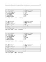
Fig. 10. Customs clearance process.
There are different types of customs clearance:
 Shipments within the European Community.
Shipments carried out in countries belonging to the European Economic Community. A
customs document is required to transport goods by sea within the geographical area of the
Economic Community.
The TL2, as it is referred to, is one single document, which once presented to and sealed in

customs, should be delivered to the shipping company’s premises within the port of
loading. The shipping company arranges the unloading of the goods into the previously
assigned vessel and sends the document to the client in the destination country. This,
together with the B/L should be sent to those responsible for unloading the goods.
 The DUA (Documento único aduanero)
Single customs document (copy) produced on green paper and containing a series of
numbered pages on which information on non-EU goods should be entered.
Each sheet has a specific purpose. For example, page three is the copy to be retained by the
person sending the document. In this case it is the customs official. With this document the
official or the forwarding agent can control the company’s turnover and in addition to
sending this to the customs officials every year, it must also be sent to Inland Revenue.
There are nine pages in total and every page has a different function.
As with the T2L, without this document the goods cannot be unloaded and transported to
their destination. Failure to pass through customs (which is necessary for the balance of
payment) before unloading goods will be treated as an offence and customs will report the
incident to the appropriate authorities and a fine will be imposed. This fine should be paid
by whomever responsible for the goods having been loaded without previous clearance.
Port terminal
at point of
origin
Customs
official
Goods
unloaded
Customs official
WAREHOUSE
Green
Red
CUSTOMS CLEARANCE

Supply Chain Management - New Perspectives
308
Moreover, under normal circumstances the goods are returned to the port of origin. Once
they are cleared by customs they can be loaded once again.
3.3 Transport company´s decision making process
The transport company’s decision making process is similar to that of any other
intermodaltransportation operator (see Figures 11 and 12).
Fig. 11. Transport company’s decision making process regarding transportation by land
between the rail or port terminal.
The company aims to meet customer demand and considers service quality their number
one priority. Enabling factors for ensuring quality service are:
 Regularity.
 Frequency.
 Flexibility.
 Availability.
The transport company offers a wide range of business services, thus providing the client
with a better service and maintaining costs as low as possible.
They must take into account the selected route and the transportation modes available. They
will then have to study the quotes received from the operators able to participate in the
transportation chain. If we assume that we are dealing with the most extensive intermodal
transportation chain in which sea, land and rail carriages are included, the operators which
may participate are the same as before: the forwarding agent, the rail and shipping
company. Each one puts forward a different quotation and the company will decide which
one most suits their needs.
DESTINATION
FREIGHT
TERMINAL
TRANSPORTATION BY ROAD:
Rail Terminal- Port Terminal
Transport

company
Rail company
Shipping
company
Forwarding
agent
Own fleet
Subcontract
PORT
TERMINAL OF
ORIGIN
Shipping
company
Own fleet
Rail company
Transport agency
Transprt agency
Shipping
company

Development of a Cost Model for Intermodal Transport in Spain
309

Fig. 12. Transport agency’s decision making process within the intermodal transportation
chain.
A detailed study of all the quotations is carried out, bearing in mind the following:
 The selected operator(s) is able to comply with the established timetables and
schedules, i.e., the frequency of services set out by the company.
 Reliability in terms of continued compliance with schedules, avoiding changes and
delays. This is important as interrupting the intermodal chain will incur losses.

 The cost of the service provided and amount saved by choosing one or the other.
Goods may be transported by land using the company’s own fleet or by subcontracting the
service to another transport company, depending on whichever option is most suitable. If
goods need to be transported by sea and/or rail, this may be done by the shipping company
or the rail company respectively.
With respect to customs clearance, the companies may take care of this by themselves if they
are certified to do so. If this is not the case, they should contact a forwarding agent who can
carry out the necessary procedures.
TRANSPORT
AGENCY
Own fleet
Contract
Rail connection?
Road carriage
only ?
1st stage
Rail
carriage
Final
stage
Own fleet
Forwarding agent
Renfe
Forwarding agent
Sea Connection ?
1st stage
Intermediary
stage
Transport company/subc
.

Forwarding agent
Renfe
Forwarding agent
Rail
transportation
Final
stage
Forwarding agent
Transport company/ Subc.

.
Forwarding agent
Sea
transportation
RECIPIENT

1)

2)

3)
1)
2
)
3)
4)
5)
Renfe
Renfe
Shipping company

Shipping company
Transport agency/Subc.
.
Forwarding agent
Renfe
Shipping company

Shipping company
Subcontracted
company
Subcontract
Own fleet
Forwarding agent
Renfe
Subcontract
Shipping company

Supply Chain Management - New Perspectives
310
4. Case study
To test our decision-making model, we applied it to a transport company located in Seville,
in the south of Spain, managing intermodal shipments from the local port and intermodal
rail terminal. The Port of Seville is located 80 kilometres from the mouth of the river
Guadalquivir, and is the only commercial inland port that exists in Spain. Its geographical
location is perfect for access from both the Mediterranean and Atlantic, with several factors
that position it as a first-rate logistical and commercial node. Traffic at the Port of Seville is
around five million tonnes annually (Table 1). Regular lines stand out with the Canary
Islands for container and ro-ro traffic, which makes the Port of Seville the main maritime
gate between the Canaries and the Iberian Peninsula.

2008 2009 2010
Goods (Tn)
4,584,671 4,504,647 4,365,589
Containers
130,452 129,736 152,612
Boats
1,278 1,242 1,181
Passengers
166,990 149,646 123,025
Table 1. Traffic at the port of Seville.


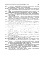
Fig. 13. Movement of freight in Spain, France, Germany and Italy on each transport mode
for year 2008.
With respect to rail transport, whereas the total amount of freight moved in Spain is
comparable to other European countries, the amount of freight moved by train is
significantly lower (see Figure 13 and Figure 14). Specifically, the modal distribution of
freight transport in Spain is as follows: road: 82%; water: 12% (and this mainly due to the
shipments to the Spanish islands, with a negligible relevance of short sea shipping); rail: 4%;
pipeline: 1.97%; air: 0.03%. Moreover, while the increase in the amount of freight on roads is
steady, rail-based transport has shown little or no increments in the recent years.

Development of a Cost Model for Intermodal Transport in Spain
311


Fig. 14. Movement of freight in Spain, France, Germany and Italy on each transport mode
for year 2009.
The only rail operator in Spain is Renfe, the national railway company. Renfe operates a

freight division, where other shippers or carriers of general freight may subcontract the
delivery of a less-than-wagon load or a whole wagon for a container. The network of freight
terminals distributed throughout Spain is depicted in Figure 15.


Fig. 15. Freight terminals operated by Renfe in Spain.

Supply Chain Management - New Perspectives
312
The intermodal shipments run by the company during the two-month period selected for
the case study are shown in Tables 2 and 3.

Distance
(miles)
Time
Taken
(days)
Time
Expected
(days)
Distance
(miles)
Time
Taken
(days)
Time
Expected
(days)
Distance
(miles)

Time
Taken
(days)
Time
Expected
(days)
1134
21 6
1504
11 5
540
30
1134
14 6
1504
14 5
540
30
1134
11 6
1504
14 5
540
17
1134
10 6
1504
14 5
540
22

1134
10 6
1504
11 5
540
31
1134
10 6
1504
9 5
540
18
1134
14 6
1504
14 5
540
22
1134
10 6
1504
18 5
540
30
1134
14 6
1504
14 5
540
30

1134
11 6
1504
14 5
540
17
1134
21 6
1504
14 5
540
22
1134
21 6
1504
14 5
540
31
1134
11 6
1504
14 5
540
18
1134
14 6
1504
14 5
540
22

1134
11 6
1504
14 5


1134
9 6
1504
13 5


1134
14 6
1504
14 5


1134
11 6
1504
11 5


1134
13 6
1504
10 5

1134
11 6
1504
10 5


1134
10 6
1504
10 5


1134
10 6
1504
10 5


1134
14 6
1504
14 5


1134
11 6
1504
18 5

1134
11 6
1504
10 5


1134
10 6
1504
10 5


1134
14 6
1504
10 5


1134
15 6
1504
17 5


1134
14 6
1504
14 5

1134
11 6
1504
10 5


1134
14 6
1504
32 5


1134
10 6
1504
11 5


1134
11 6
1504
14 5


1134
14 6
1504
10 5

1134
14 6
1504
10 5


1134
14 6





Table 2. Data on the intermodal waterborne shipments delivered by the case-study
company.

Development of a Cost Model for Intermodal Transport in Spain
313
Distance
(Km)
Time
Taken
(days)
Time
Expected
(days)
Distance
(miles)
Time
Taken

(days)
Time
Expected
(days)
1099
2 1,5
570
3 1
1099
2 1,5
570
2 1
1099
2 1,5
570
3 1
1099
2 1,5
570
2 1
1099
2 1,5
570
4 1
1099
10 1,5


1099
2 1,5

1099
2 1,5


1099
2 1,5


1099
3 1,5


Table 3. Data on the intermodal rail shipments delivered by the case-study company
4.1 Cost data
In order to represent the decision-making process of companies involved in intermodal
transport, we gathered all the cost-related data for each link of the intermodal chain. This
included vehicle cost components, rail and ship tariffs, intermediary supplements, etc. The
data collection was carried out by accessing the appropriate statistical sources in each case,
or by direct consultation to the involved stakeholders.

4.1.1 Road transport
The Spanish Ministry of Public Works publishes a yearly report (Ministerio de Fomento,
2009) for road transport companies providing them with reliable criteria upon which they
may establish the price of the service offered. This publication contains average cost data
related to the different concepts involved in road transport, and has become a capital
reference for the establishment of transport rates in the country. An example of the type of
data provided is shown in Table 4. The cost data was then translated into prices by adding
the average commercial margins in the sector.

4.1.2 Rail transport
Every year the rail company Renfe offers its clients rates depending on the origin and
destination terminal. The rates data for haulages departing from Seville is shown in Table 5.
On top of these rates, clients must pay a surcharge for the different additional services (road
haulage, container storage, etc.) offered by Renfe.
4.1.3 Waterborne transport
The rates charged for the waterborne transport of a container correspond to the transport
itself, which is often negotiated between the shipper and the carrier, plus the port charges.
The concepts normally included in a vessel transport invoice are:

Supply Chain Management - New Perspectives
314

ANNUAL DIRECT COSTS
Euros Distribution (%)
Direct costs
119,420.84 100.0%
Costs per time
65,274034 54.7%
Vehicle depreciation
13,844084 11.6%
Vehicle financing
1,302.69 1.1%
Drivers
28,384073 23.8%
Insurance
6,848.08 5.7%
Tax costs
928.00 0.8%
Expenses

13,966.00 11.7%
Kilometric costs
54,146.50 45.3%
Fuel
41,619.83 34.9%
Tyres
6,730.67 5.6%
Maintenance
2,088.00 1.7%
Repairs
3,708.00 3.1%
Annual distance travelled (km/year) 120,000
Annual distance travelled for loaded vehicles (km/year) 102,000
Direct Costs (euros/km covered) 0.995
Direct Costs (euros/km covered by loaded vehicle) 1.171
Table 4. Average cost data for a vehicle containing a normal load (420 HP, MAM = 40,000kg
and payload of 25,000kg). Base hypothesis: 20,000 km covered every year, 85% loaded and
15% empty. (Source: Spanish Ministry of Public Works).
 The haulage rate (BAS) for sea transportation and the previous procedures associated
with ship operations.
 Obtaining the necessary currency for payment of freight.
 THC for handling of goods in port terminals. This is called the OHC in the terminal of
origin and DHC in the terminal of destination.
 The goods rate (PTD) for use of port facilities. This depends on the weight of the goods
and the container.
 Management of the consignee (shipping company) for port operations between them
and the forwarding agent, the customs official, recipient/shipper, port terminal and
carrier. This involves the notification of arrival, the B/L (bill of lading) and the delivery
and acceptance order. A sum is paid for the processing of documents. In the origin this
is called the ODF and in the destination the DDF.

 Management of the Customs official for goods clearance procedures (presentation of
DUA, customs release, closing of DUA, and/or presentation of additional
documentation, physical inspection, representation and obtaining of customs release -
document or physical inspection) which will be explained later.
 IHE Inland Haulage Export (TTE)/Import (TTI).
 Warranty of article 102: warranty to respond as a whole to deferment of payment of the
customs debt in accordance with the Customs Code.
 BAF. This is the amount to be paid depending on the cost of fuel.
 CCN is the surcharge for cleaning the container (this varies according to terminal).
 Occupancy: this is the amount to be paid for temporary storage of goods in the terminal
port and for any delays caused as a result of container occupancy.

Development of a Cost Model for Intermodal Transport in Spain
315
LOADED EMPTY
DESTINATION CH
20' <12
Tonnes
20'> 12
Tonnes
30'

40'

20'

30'

40'

A CORUÑA S.D. * 404.2 504.21 615.29 779.75 270.02 403.05 452.37
BARCELONA
MORROT
* 410.74 514.19 625.19 792.22 274.38 409.52 459.54
BILBAO PORT * 376.79 477.74 558.96 703.34 262.19 377.92 423.86
GIJON PORT * 370.3 467.5 577.57 686.53 263.77 378.98 428.72
IRUN * 368.56 452.52 560.77 710.33 246.66 367.95 412.72
JUNDIZ * 340.21 439.61 517.54 655.63 227.72 339.82 381.03
LEON * 316.97 388.88 469.22 591 229.29 328.51 375.74
MADRID
ABROÑIGAL
178.92 224.45 272.39 344.91 119.11 177.41 199.14
MURIEDAS * 340.21 439.61 517.54 655.63 227.72 339.82 381.03
NOAIN * 367.19 448.1 546.68 688.36 263.39 379.43 430.92
SILLA * 266.53 375.62 405.32 517.54 178.24 265.54 298.12
TARRAGONA
CONSTANTI
* 383.11 479.12 582.37 738.67 280.76 382.69 429.29
VALLADOLID
ARGALES
* 238.61 299.32 356.45 452.01 177.44 245.92 275.79
VIGO GUIXAR * 380.01 473.94 578.56 733.09 254.38 379.72 426.02
ZARAGOZA * 346.42 423.33 525.11 668.36 370.74 370.74 446.86
Table 5. Price rates for containers leaving the Seville intermodal terminal on a Renfe train
(CH: Container Hire) (Source: Renfe Combined Transport Rates).
The invoice may have a different layout depending on the shipping company. However, the
concepts included are more or less the same as those outlined above. Below we have an
example (Table 6) of a Spanish port invoice for a 20’ dry container:

Port invoice (euros)

BAS
400/600
BAF
30/50
OHC
140.04
DHC
140.04
PTD
30
ODF
45
DDF
45
CCN
6
FFC
2.5
Carriages
- Internal port
62
- 0-10km
100
- over 200
1.03 cents/km
Table 6. Example of a port invoice for a 20’ dry container (€).

Supply Chain Management - New Perspectives
316
Other concepts are included in the invoice but indirectly. These are the services provided

directly or indirectly by each Port Authority.
 Direct Services are those services provided to the ship or goods (in accordance with the
BOE, Official Gazette of the Spanish State).
 Indirect Services are those provided to the ship or goods by the Port Authority through
individuals or third parties (subcontacted or by means of concession).
We will now look at the different components of this service and their corresponding rates,
all of which will be looked at with reference to the Port of Seville.
4.1.3.1 Direct services
 Ships accessing the port, berthing or anchoring:
 The rate is 0.04912 euros/GT for short stays of 3 hours (maximum of 4 periods every 24
hours) Reductions are applicable for the use of facilities under administrative
concession, for lack of draught in berthing, mooring method and navigation type
(cabotage between ports within the European Union).
 For the number of stopovers made (Table 7):
 For long stays a minimum surcharge of 0.009196 and a maximum of 0.055173 euros per
GT and day of stay is applied.

Generally Applied Reductions
From 13 to 24 stopovers 20%
From 25 to 40 stopovers 45%
From 41 stopovers 70%
Reductions for scheduled routes
From 13 to 24 stopovers 5%
From 25 to 50 stopovers 15%
From 51 to 100 stopovers 25%
From 101 stopovers 35%
Table 7. Applied reductions for the number of stopovers made.
 Goods. Rates for general goods per section (Table 8):

Discount

group
% disc. *
Amount discounted (€/Tonne)
UNLD Base LD
First
85 0.565552 0.459774 0.354056
Second
75 0.942567 0.766290 0.590074
Third
60 1.508059 1.226065 0.944070
Fourth
30 2.639104 2.145613 1.652122
Fifth
0 3.770149 3.065162 2.360175
UNLD=Unloading LD=Loading
*Based on the basic amount of 3.065162 €/Tonne
Table 8. Rates for general goods per section.
 Other services. Scales:
 For lorry: €1.664804

Development of a Cost Model for Intermodal Transport in Spain
317
 For loaded wagon: €5.709615
 For empty wagon: €3.305567
4.1.3.2 Indirect services
Pilotage: Services to facilitate entry to and departure from the port and manpower within
the boundaries where such activity takes place. According to National Ports Authority Law,
Merchant Navy regulations and the General Regulations of Pilotage, Some of the discounts
applicable are:
 For ship type:

 Passenger and Ro-Ro ships: 5%
 Scheduled Ro-Ro ships: 8%
 Scheduled Ro-Ro ships which stopped at Seville before 01/06/99 and whose GRT
was less than 3000 and GT more than 6000 units: 13%
 Scheduled routes:
 More than 40 annual stopovers: 47%
 More than 24 annual stopovers: 35%
 More than 10 annual stopovers: 20%
 Ships who berth outside the dock: 20%
5. Results and conclusions
5.1 Assessment of the company’s operations
After having applied the decision-making model to the company's intermodal routes, (road-
rail-sea and road-rail), the following observations can be made:
 Road-rail-sea-route: Although the decisions taken illustrate how the model may be
most effectively implemented, they do not reduce costs. The company is not 100%
efficient, since the initial road carriage is subcontracted. The least expensive option is to
contract this through Renfe, provided that they also manage the rail carriage. As our
results have shown, contracting Renfe for the road carriage would be less expensive
than using the company’s own fleet, at least for the first 70 km. Besides, if as a result of
the liberalisation of the rail market, Renfe loses its monopoly in this sector, the market
will be more competitive and costs will be reduced. In this way, having the rail operator
manage the road carriage, as indicated by the model, will be less expensive.
 Road-rail route: The company has been able to optimise the costs incurred in this route
by implementing the decision-making model and has therefore made the right decision.
The figures show that using intermodal transport, rather than road transport only,
considerably reduces costs by 50%, which confirms that intermodal transport is more
cost-effective than road for distances greater than 500 km.
Besides, in addition to making its business more economically efficient, the company also
aims to maintain customer loyalty and service quality. The introduction of intermodal
transport therefore widens the range of services offered to its clients and as new routes

open, the incorporation of other services is also possible. As borders are opened up, the
company is able to reach other destinations that were previously limited to road transport.
5.2 General conclusions for intermodal transport in Spain
Besides using the developed model to assess the specific intermodal operations of the case-
study company, it was also used to analyse transport routes from Seville to the rest of Spain.
Depending on the location of intermodal terminals throughout the national territory, and on

Supply Chain Management - New Perspectives
318
the distances to these terminals and from Seville, it was possible to determine which
transport option would be cheapest for hauling a container from Seville to all the other
Spanish provinces.
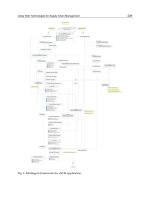
The result is shown in Figure 16, and comes to confirm the generally accepted statement that
intermodal transport is only cost-effective for distances longer than 500 km. In the case of
Spain, road transport to the East coast would still be the preferred option due to the
existence of a highway along the coast, while rail shipments have to pass through Madrid. It
is also significant to mention that, even though waterborne transport is only cost-effective
for shipments to the islands, it is the second cheapest option, after rail transport, for
shipments from Seville to the coastal areas in the north of Spain.
It has been noted that in long distance and intercontinental routes, although the use of
intermodal transport improves the relationship between time taken and distance covered, it
may also have a negative impact due to periods of unproductivity when goods are
stationary and the mode used for the carriage is unavailable. It is therefore necessary to
dedicate resources to avoiding any negative impact from factors such as these. For example,
this can be done by improving data exchange and compatibility between the different
agents’ schedules, among others.
Although intermodal transport is much more developed in other countries than in Spain, as
time passes and borders are opened up and the market becomes more global, intermodal
transport may establish itself as the most efficient solution, thus making it much easier for
small and medium enterprises to enter the market.

Fig. 16. Cost-effectiveness borders for the different transport modes in Spain for shipments
from Seville, as obtained from the decision-making model.

Development of a Cost Model for Intermodal Transport in Spain
319
5.3 Effect of additional factors

The analysis was also be extended to other non-monetary effects, such as time and shipment
reliability, which play a very important role in making the road more attractive to freight
transport than other alternative modes (Modenese Vieira, 1992). One of the objectives of the
paper was thus to gain some insight about the importance of these non-monetary effects on
the decision-making process related to intermodal transport, as it might sometimes be
cheaper than road transport but is also often less reliable. Two additional factors were
considered in the analysis:

 The time taken for the delivery, measured as average of time taken. (Table 9 and 10)
 The reliability of the delivery, measured as standard deviation of the time taken. (Table
9 and 10)

Distance (miles) Time Expected (days) Time average (days) Standard deviation (days)
1134
6 12,72 3,09
1504
5 13,24 4,07
504
24,29 5,73
Table 9. Data analysis on the intermodal waterborne shipments delivered by the case-study
company.

Distance (Km) Time Expected (days) Time average (days) Standard deviation (days)
1099
1,5 2,90 2,51
570
1 2,80 0,84
Table 10. Data analysis on the intermodal rail shipments delivered by the case-study
company.
The procedure followed consisted in registering data on the intermodal shipments delivered
by the case-study company (Table 9 y 10).
In terms of the time taken for deliveries, the high values of the time average of the
waterborne case may be explained by the fact that it includes an intercontinental route, and
therefore rotations are higher due to port of calls and procedures for entering port areas. As
a result, although the distance covered is less than other routes, the time taken is greater. It
may also be due to the time taken to load and unload in the port of destination. In the case
of rail transport, the time average values are greater than time expected but not as the
waterborne case.
In terms of reliability, the data for waterborne transport shows an increased standard
deviation with the distance of the trip, international case except for the reasons previously
exposed. In the case of rail the trend is the same, which highlights the fact that unexpected
delays take place in the distance between origin and destination, and are therefore
independent of terminal operations rather than during the movement process itself.
The standard deviation is high. This means that time and reliability vary a lot over the same
distance. It would have been useful to look at more routes; however, no more data was
available, so the results are not very reliable. However, this type of analysis is useful since it
allows us to measure the importance of these additional factors in intermodal transport.
With more data, more sophisticated analysis may be carried out and more reliable data
obtained.

Supply Chain Management - New Perspectives

320
6. References
Arnold P., Peeters D., & Thomas I. Modelling a rail/road intermodal transportation system.
Transportation Research Part E-Logistics and Transportation Review, Vol. 40, No. 3,
(May 2004), pp. 255-270,

1366-5545.
Ballis A., & Golias J. Towards the improvement of a combined transport chain performance.
European Journal of Operational Research, Vol. 152, No. 2, (January 2004), pp. 420-436,
0377-2217.
Barthel F., & Woxenius J. Developing intermodal transport for small flows over short
distances. Transportation Planning And Technolog, Vol. 27, No. 5, (2004), pp. 403-424,
0308-1060.
Cuerda J.C., Fernández M.J., Larrañeta J., Muñoz S., Sánchez F., & Vélez C. (2003).
Environmental policy and environment-oriented technology policy in Spain, In:
Environmental and Technology Policy in Europe, Geeerten J.I.S., & Sedlacek S., pp. 163-
196, Kluwer Academic Publishers, 1-4020-1583-6, Netherlands.
Dirección General de Programación Económica. (2004). “Encuesta Permanente de Transportes
de Mercancías por Carretera (EPTMC)”, Ministerio de Fomento.
Li L., & Tayur S. Medium-term pricing and operations planning in intermodal
transportation. Transportation Science, Vol. 39, No. 1, (February 2005), pp. 73-86,
0041-1655.
Macharis C., & Bontekoning Y.M. Opportunities for OR in intermodal freight transport
research: A review. European Journal Of Operational Research, Vol. 153, No. 2, (March
2004), pp. 400-416, 0377-2217.
Ministerio de Fomento. (2006). Observatorio de mercado del transporte de mercancías por
carreteras. Centro de Publicaciones, Secretaría General Técnica.
Modenese Vieira L.F. (1992). The value of service in freight transportation. PhD thesis.
Massachusetts Institute of Technology.
Observatoire des politiques et des stratégies de transport en Europe. (2005). “Dossier n°7: Le

transport intermodal en Europe”, Conseil National des Transports (CNT).
Ramstedt L., & Woxenius J. (2006) Modelling approaches to operational decision-making in
freight transport chains. Proceedings of the 18th NOFOMA Conference, Oslo, June
2006.
Walker W.E., van Grol H.J.M., Rahman S.A., Lierens A., & Horlings E. Improving the
intermodal freight transport system linking Western Europe with central and
Eastern Europe - Identifying and prioritizing policies. Transportation Research
Record, Vol. 1873, (2004), pp. 109-119, 0361-1981.
0
Location Problems for Supply Chain
Feng Li
1
, John Peter Fasano
2
and Huachun Tan
3
1
IBM Research - China
2
IBM Thomas J. Watson Research Center
3
Beijing Institute of Technology
1,3
P. R. China
2
U. S. American
1. Introduction
A typical supply chain is a materials and information network composed by supplier,
manufactures, logistics agencies, distribution center, warehouse, retailer and consumer. It
involves all enterprises and departments throughout the whole product life-cycle from

the material gaining, production to semi-finished products or finished products, assembly,
transportation, consumption till disposal. Supply chain management is the term used to
describe the management of the flow of materials, information, and funds across from
those enterprises and departments. It has been proved to be an effective way to enhance
enterprises’ adaptive ability and viability in the market by collaborating with the upstream
and downstream enterprises in the competitive market.
Traditionally, location problem is a branch of operations research concerning itself with
mathematical modeling and solution of problems concerning optimal placement of facilities
in order to minimize transportation costs, avoid placing hazardous materials near housing,
outperform competitors’ facilities, etc. Location problems in supply chain management is to
find the ideal locations for suppliers, manufactures, distribution centers and warehouses to
achieve different objectives by using mathematical modelling, heuristics, and mathematical
tools such as, ILOG CPLEX, LogicNetPlus etc.
With the increased environment pollution concerns of people, organizations and
governments, enterprises are facing pressure to protect and improve the environment, such
as decreasing environment pollution, reducing waste cites and using green raw material etc.
In order to solve this problem, enterprises begin to integrate Supply Chain Management
(SCM) with the thought of environment protection. With the development of researches on
this problem, it naturally comes green supply chain management Stevels (2002). Presently,
green supply chain management are mainly focused on the following two aspects: 1)
green technology, such as green design, green manufacturing and remanufacturing, waste
management, and green logistics and green management Wang et al. (2005). 2) green materials
flow, it is to make material flow effective and green by the management of material flow, for
example, using green materials, recycling disposal products etc Srivastava (2007). Among
those technologies, the approaches for location problems play key roles in green supply chain
management.
15
2 Will-be-set-by-IN-TECH
Motivated by the above problems, we will firstly review the traditional location problem in
supply chain management from the following three views: modelling, solving algorithms

and mathematical tools, then we will demonstrate the development of location problem in
supply chain and propose mathematical model for distribution center location problem in
green supply chain. Finally we will illustrate the proposed problem by using IBM Watson
Implosion Technology.
2. Literature review
Location theory was first formally introduced in 1909 by Alfred Weber, who considered
the problem of deciding a location in the plane to minimize the sum of distance from the
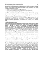
distribution center to all demand consumers/retailers. A typical location problem and its
solutions are shown in the following two figures. Obviously, the above problem can be
(a) Facility Location Problem (b) Solution for Facility Location Problem
Fig. 1. Facility Location Problem and Its Solution
described as following mathematical model:
Geometric Solution = arg min
y∈R
n
12
∑
i=1

x
i
− y

2
(1)
Where x
1
, x
2
, ··· and x

12
are the points where the twelve customers locate, y is position where
the facility located.
Based on the simple model provided by Alfred Weber, researchers had proposed lots of
models to describe complex location problems for different industries. In fact, location theory
is not only a pure mathematical problems, it comes from application, and it also has lots
of applications in different industries, such as logistics, public fire protection, manufacture
etc. For example, when a supply retailer is thinking to open a new outlets, he will consider
customer demands and related costs for different locations. When a manufacturer chooses
where to position a warehouse, he will consider customer demand, cost, inventory and cost
and market trends of targets locations. When a city planner selects locations for fire stations,
he will consider the requirements and constraints for fire fighting. Obviously, those problems
are typical location problems.
322
Supply Chain Management - New Perspectives
Location Problems for Supply Chain 3
Although all of those problems are called as location problems, there are many difference
in constraints and objectives. Those constraints and objectives are coming from
factors/decisions for specific industries Li et al. (2007). For different industries, the
factors/decisions are different. For instance, customer demand, population shift and market
trends evolve will be considered for a logistics planner when he determine the location for
distribution center, minimum transportation time and district coverage rate will be thought
for a city planner when he selects locations for fire stations. Because those factors will have
impact on the constraints of location model, they will result in lots of challenges for models
and algorithms for location problems. According to the objectives of those problems, we can
classify those problems as the following six groups,
1) Minimize average travel time/average cost or maximize of net income,
2) Minimize average response time,
3) Minimize maximum travel time/cost,
4) Minimize maximum response time,

5) Maximize minimum or average travel time/cost,
6) Problems with other objectives.
According to the characteristics of those problems, we can identify them as, static and
deterministic location problems, dynamic location problems and stochastic location problems.
Distribution center location is a typical location problem. Choosing the proper location for
a distribution center has developed into a specialized, scientific process. Cost and non-cost
factors such as efficient customer access, infrastructure availability, proximity to qualified
labor, variable operating costs, incentive availability, and environmental impact are all part
of the scientific equation. As a supply chain planner begins the location selection process, the
following two questions are very important for him:
1. What are the factors that will control the supply chain decision?
2. What are the steps to properly select a location?
Transportation, the largest location-dependent cost factor, is addressed first. After
transportation, labor cost/ productivity, quality, work ethic, and supply, available or
develop-able land, power needs, water and waste water supply and capacity, and building
costs are considered. Moreover, as basic energy costs have continued to rise, utility costs
have become a more important element in the site selection process. Besides those factors,
inventory and services costs will also be taken into accounts. When we determine the locations
of its distribution centers for a green supply chain, we will consider the other important factor,
carbon emissions, besides those factors mentioned above.
2.1 Models for location problem
In order to formulate this problem mathematically, the following notations are necessary:
Inputs:
i
= index of customer,
j
= index of potential location for distribution center,
k
= index of manufacture,
R

i
= product requirement for customer i,
P
i
= sale price for customer i,
323
Location Problems for Supply Chain
4 Will-be-set-by-IN-TECH
I
j
= maximal inventory for potential distribution center location j,
C
o
j
= total cost for opening a distribution center at location j,
C
p
k
= production cost of manufacture k for single product,
C
ij
= transportation cost from location j to customer i for unit product,
¯
C
jk
= transportation cost from manufacture k to location j for unit product,
Decision Variables
x
j
=


1, if open a distribution center at location j,
0, otherwise.
y
ij
= product transport volume from j to i,
z
jk
= product transport volume from k to j,
Using these definitions, the model for distribution center location can be described as follows,
max
∑
j

∑
i
(P
i
− C
ij
)y
ij
− C
o
j
x
j
−
∑
k

(
¯
C
jk
+ C
p
k
)z
jk

s.t.
∑
j
x
j
· y
ij
= R
i
, ∀i,
∑
i
y
ij
−
∑
k
z
jk
≤ 0, ∀j, (2)

∑
k
z
ij
− x
j
· I
j
≤ 0, ∀j,
x
j
∈{0, 1}, y
ij
≥ 0, z
jk
≥ 0, ∀i, j, k.
In model (2), the first constraint is to satisfy each customer demand, constraint from is to meet
the requirement that the supply volume of the product at each distribution center should be
greater than the demand volume of the product, the third constraint is to limit the total stock
volume less than the maximal inventory of each distribution center, the forth constraint is to
restrict the decision variable x
j
be0or1.
2.2 Algorithms for location problem
In order to solve those problems, the researchers also proposed dozens of exact optimization
algorithm and heuristics Brandeau & Chiu (1989); Owen & Daskin (1998); Rosing (1992).
The most popular used exact optimization algorithms go as follows, branch-and-bound,
branch-and-cut, column generation, and decomposition methods. Where branch-and-bound
algorithms sometimes combined with Lagrangian relaxation or heuristic procedures to obtain
bounds.

Normally, static and deterministic facility location problems are attractive to be solved by
exact optimization algorithms. However, in the real world, the number of decision variables
is large and the models are comparatively more complex, it is hard to obtain optimal
solution by exact optimization algorithms. There comes the heuristic method. Lagrangian
relaxation, linear programming based heuristics and metaheuristics are among the most
popular techniques. In fact, most of time the dynamic location problems, stochastic location
problems and problems with multiple objectives can only be solved with some specific
methodology, heuristics. At the same time, researchers had created and built some useful
and innovative tools to help us solve the location problem in supply chain.
324
Supply Chain Management - New Perspectives
Location Problems for Supply Chain 5
2.3 Tools for location problem
The most famous tools for the location problems is IBM ILOG LogicNet Plus XE and Watson
Implosion Technology. Below we will illustrate them one by one.
2.3.1 IBM ILOG LogicNet Plus XE
IBM ILOG LogicNet Plus XE is a software for supply chain network optimization and supply
chain design, an off-the-shelf decision support solution for ongoing strategic planning. It
is for network design and production sourcing. It determines the optimal number, location,
territories, and size of warehouses, plants, and lines. It also determines where products should
be made and optimizes the carbon footprint. Figure 2 give a typical case for using IBM ILOG
LogicNet Plus XE.
Fig. 2. Typical Case for ILOG LogicNet Plus XE
IBM ILOG LogicNet Plus XE can solve the following typical applications:
1. Distribution Network Design, Determine the optimal number, location, and size of
distribution facilities to meet customer service requirements at minimum cost.
2. Manufacturing Network Design, Determine the best number, location, and capacity of plants,
lines, and processes to maximize asset utilization, minimize total cost, and align capacity
with business growth projections.
3. Manufacturing Sourcing Strategy, In a multiplant environment, determine which product

should be made at which plant, trading off manufacturing costs and economies of scale
with transportation costs.
4. Shipping Territory Realignment, Determine the best service territory for each DC
(Distribution Center) to improve service levels and reduce costs.
5. Network Transition Planning, Make the transition to a new supply chain configuration
focusing on various asset, capacity, inventory and transportation lane requirements.
6. Seasonal Supply Chain Design, In a highly seasonal business, determine the appropriate
trade-off between capacity and inventory prebuild and the use of overflow facilities.
7. Contingency Planning, Understand how unexpected events in the supply chain will affect
the costs, service levels, and potential revenues. Develop plans to mitigate the risks.
The major inputs for this tool includes
1. Customer locations and demand by product and time period.
325
Location Problems for Supply Chain
6 Will-be-set-by-IN-TECH
2. Locations, costs, and capacities for plants, suppliers, and production lines for existing and
potential sites.
3. Locations, costs, and capacities of existing and potential warehouses.
4. Transportation costs for each lane.
5. Service level requirements.
6. Carbon emissions data.
7. Tax rates.
Fig. 3. Screen Shot for ILOG LogicNet Plus XE
Figure 3 is a screen shot for the tool of IBM ILOG LogicNet Plus XE. It will help you to build
supply chain for your problem by tables. By using those tables, we can input the data and their
relationships for products, by-products, bill of materials, plants, warehouses (distribution
centers), customers, transportation, and taxes etc. Once we’ve finished building the model,
we can click on the "Optimize" button to obtain solution for our problems. Integrating with
geographic information map, the tool can help us to review the solution through a map. It
will visualize the locations for the customer, plants, and distribution center (warehouses).

The tool also provide summary report for the solution, including the various input and
output parameters for the latest optimization run, such as run time, optimization gap, and
the total cost of the solution. This report also has sections on financial summary, cost totals,
transportation summary, variable cost details, holding cost details, and manufacturing cost
details. Meanwhile we can use the tool to do sensitivity analysis for the model by adjusting the
parameters of the model. Although IBM ILOG LogicNet Plus XE has powerful function and
can solve several kinds of problems in supply chain management, it cannot support graphical
mode to build models.
326
Supply Chain Management - New Perspectives
Location Problems for Supply Chain 7
2.3.2 Watson Implosion Technology
Watson Implosion Technology (WIT) tool is a graphical modeling tool Wittrock (2006), it was
generated to solve particular kind of production planning problem, especially for constrained
materials management and production planning problem. It utilizes an analytical decision
making approach to determine if equipment is worth selling as whole or if it should be
dismantled for service parts, which can often yield better returns. It can describe the
planning problem as an optimization model by using visual predefined components, and the
optimization model will further calculate the number of products to disassemble in a given
time period to fulfill the demand for various components. A typical WIT model is should as
following Figure 4
Fig. 4. Typical WIT Model
Table 1 defines all of the manufacturing terms for WIT. The primary data for this software
tool is a list of demands for products, a list of supplies for components, and a multi-level
bill-of-manufacturing (BOM) describing how to build products from components. Ordinarily,
it takes many components to build a single product, and so the list of supplies is much
larger than the list of demands. A traditional use of a BOM to perform production planning
is Material Requirements Planning (MRP), in which the list of demands for products is
"exploded" (via the BOM) into a much larger list of requirements for components. The main
capability provided by WIT is, in some sense, the reverse of an MRP explosion: the WIT

"implosion". The list of supplies of components is "imploded" via the BOM into a relatively
small list of feasible shipments of demanded products. The assumption is that not all demands
can be met, and therefore the idea is to make judicious trade-offs between the different
demands given limited supplies to best satisfy the manufacturing objectives.
In general, optimizing implosion is used to find the best possible implosion solution according
to some well-defined criterion. We can use WIT tool to determine the best possible distribution
327
Location Problems for Supply Chain
8 Will-be-set-by-IN-TECH
Period The time bucket for production plan.
Part WIT’s concept of a part is very general. A part is either a product or
anything that is consumed in order to build a product. This includes
both materials and capacities.
Part Category Parts are classified into two categories: Material and Capacity
Operation An operation is the means by which parts are dismantled. Specifically,
a part is dismantled by "executing" an operation. When an operation
is executed, some parts (machines) are consumed, while other parts
are produced.
Material A material part is either a raw material or a product. Any quantity of
a material part that is not used in one period remains available in the
next period. In other words, material parts have stock.
Capacity A capacity represents some limitation on the quantity of one or more
operations that can be executed during one period. We assume no
capacity limitation at dismantling or refurbish centers.
BOM (Bill-of-
Manufacturing
/Materials)
Each operation has a bill-of-manufacturing that specifies the how parts
(both material and capacity) are consumed when the operation is
executed. In MRP terms, this is roughly equivalent to a combined

bill-of-material and bill-of-capacity.
BOM entry A BOM entry is the association between a particular operation and
one particular part in its BOM. Each BOM entry represents the
consumption of some volume of a part in order to execute some
operation.
BOP (Bill-of-
Products)
Each operation has a bill-of-products that specifies the how parts are
produced when the operation is executed. Production rates indicating
how much of the part is produced, and so on.
BOP entry A BOP entry is the association between a particular operation and one
particular part in its BOP. Each BOP entry represents the production of
some volume of a part as a result of executing some operation.
Product Any part that appears as the produced part of a BOP entry.
Demand Each material part may optionally have one or more demands
associated with it. A demand stream represents an external customer
who places demands for the part.
Table 1. Definition of WIT Terms
center locations and transportation modes for delivering the products given a defined set of
criteria. In the following section we will use this tool to illustrate the proposed models.
3. Distribution center location in green supply chain
The concept of green supply chain was first introduced in 1996. Since green supply chain
was given it has been getting a lot of attention. It aims to not only synthetically consider
the environment impacts and resources utilization in the manufacturing supply chain but
improve good business sense and obtain higher profits Wilkerson (2005). Green supply chain
328
Supply Chain Management - New Perspectives
Location Problems for Supply Chain 9
management involves a fundamental rethinking of supply chain management practices and
how they can be integrated with your company’s environmental strategy, such as, carbon

emission and power consumption etc.
Distribution center is a core part for a supply chain. A typical structure is shown in Fig.5,
while warehouses are distribution centers which connect factories and retailers. A suitable
distribution center location can help us reduce the transportation cost, operation cost of
the supply chain and improve the operation efficiency and logistics performances . It is a
crucial question in the design of efficient logistics systems to identify the distribution center
location Blanchard (2010). Currently choosing the proper location for a distribution center
has been developed into a specialized, business and scientific process. It will consider cost
and non-cost factors such as efficient customer assess, infrastructure availability, proximity to
qualified labor, and variable operating costs. With the increasing concerns on global warming
of environmental challenge, the decision to curtail carbon emission become more and more
serious for all of the poor and rich countries Akerlof (2006). That makes reducing carbon
dioxide emission become a key problem for green supply chain, especially for the distribution
center location problems.
)DFWRU\
:DUHKRXVH 5HWDLOHU7UDQVSRUW
7UDQVSRUW
Fig. 5. Typical Distribution Center Location Problem.
3.1 Problem statement
As shown in Fig.5, distribution center location for green supply chain is to determine several
locations for distribution centers in a supply chain while pursuing minimal operations cost,
carbon emission, maximal profits, considering inventory constraints and satisfying customer
demands.
3.2 Mathematical model
Model (2) is a typical description for distribution center location problem. It is to maximize
its profits and minimize operations costs while considering inventory and customer demand
constraints. However it has ignored an important factor for green supply chain. That’s the
carbon emission. Carbon emission is related with the manufacture and transportation. Carbon
329
Location Problems for Supply Chain

10 Will-be-set-by-IN-TECH
dioxide will be generated during the production and transportation process, and energy will
be consumed during those process. Below we do not consider how to improve the production
technology of each manufacture in order to reduce the carbon emission. We suppose the
carbon emission for producing a product are fixed for every manufacture, and they can be
different for different manufactures. Using the above notations, we can get the following
multiple objective mathematical model,
max
∑
j

∑
i

P
i
· y
ij
−
∑
m
C
m
ij
· u
m
ij

− C
o

j
· x
j
−
∑
k

C
p
k
· z
jk
+
∑
m
¯
C
m
jk
· v
m
jk


min
∑
m
∑
j


∑
k
v
m
jk
· (
¯
E
m
jk
+ V
m
· E
k
)+
∑
i
u
m
ij
· E
m
ij

s.t.
∑
j
x
j
· y

ij
= R
i
, ∀i,
∑
m
V
m
· u
m
ij
= y
ij
, ∀i, ∀j, (3)
∑
m
V
m
· v
m
jk
= z
jk
, ∀j, ∀k,
∑
i
y
ij
−
∑

k
z
jk
≤ 0, ∀j,
∑
k
z
ij
− x
j
· I
j
≤ 0, ∀j,
x
j
∈{0, 1}, y
ij
≥ 0, z
jk
≥ 0, ∀i, j, k.
where, m represent the number of types for transportation mode used to transfer product from
manufactures to distribution centers and from distribution centers to customers. u
m
ij
and v
m
jk
denote the transportation round times of mode m from the j-th distribution center to the i-th
customer and from the k-th manufacture to the j-th distribution center, respectively. C
m

ij
and
¯
C
m
jk
denote the cost of mode m for single transportation round from from the j-th distribution
center to the i-th customer and from the k-th manufacture to the j-th distribution center,
respectively. E
k
denote carbon emission for producing single product at the k-th manufacture,
respectively. E
m
ij
denote carbon emission of mode m for a round transportation from the j-th
distribution center to the i-th customer,
¯
E
m
jk
denote carbon emission of mode m for a round
transportation from the k-th manufacture to the j-th distribution center, V
m
denote volume of
mode m for single round transportation.
Model (3) is a bi-objective mathematical programming, the first objective is to maximize
the profits of the supply chain, the second objective is to minimize the carbon emission of
the supply chain. At the first glance there is no relationship between these two objectives.
In fact, these two objective are dependent. For example, if we decrease the transportation
cost, let’s say, decrease the gas consumption, we will cut down the carbon emission of the

transportation. In this paper, we will assume the the carbon emission for transportation is a
function of the transportation cost and the carbon emission for different manufacture is also a
function of the manufacture cost for that factory.
330
Supply Chain Management - New Perspectives
Location Problems for Supply Chain 11
3.3 Algorithms and experiments
Using WIT tool, It is easily for us to translate the model (2) from mathematical equations into
a visual WIT model. The WIT model is shown as Fig.6, where,
'
' '
&
&
&
:
:
3
3
F
F
F
F
'HPDQG
&XVWRPHU
7UDQVSRUWDWLRQ
:DUHKRXVH
7UDQVSRUWDWLRQ
3ODQWDQG
&DSDFLW\
2SHQ

:DUHKRXVH
2 2
7
7 7
7
7 7
7
7
7
7
Fig. 6. WIT Model for Model 2
• P1-2: products in factory, defined as materials;
• W1-2: products in warehouse, defined as materials;
• C1-3: products for customer, defined as materials;
• D1-3: demands from customer;
• T1-10: transportation defined as operation, which move products from factory to
warehouse, or from warehouse to retailer/customer;
• O1-2: open warehouse/(distribution center) defined as operation. Once a open warehouse
operation is executed, the warehouse can be used;
• c1-4: capacity, which is generated only when the warehouse is opened. Specially, it is
consumed by each transportation operation.
331
Location Problems for Supply Chain