Vibration Analysis and Control New Trends and Developments Part 6 potx
Bạn đang xem bản rút gọn của tài liệu. Xem và tải ngay bản đầy đủ của tài liệu tại đây (1.61 MB, 25 trang )
6
A Semiactive Vibration Control Design for
Suspension Systems with Mr Dampers
Hamid Reza Karimi
Department of Engineering, Faculty of Engineering and Science
University of Agder
Norway
1. Introduction
In an automotive system, the vehicle suspension usually contributes to the vehicle's
handling and braking for good active safety and driving pleasure and keeps the vehicle
occupants comfortable and reasonably well isolated from road noise, bumps and vibrations.
The design of vehicle suspension systems is an active research field in automotive industry
(Du and Zhang, 2007; Guglielmino, et al., 2008). Most conventional suspensions use passive
springs to absorb impacts and shock absorbers to control spring motions. The shock
absorbers damp out the motions of a vehicle up and down on its springs, and also damp out
much of the wheel bounce when the unsprung weight of a wheel, hub, axle and sometimes
brakes and differential bounces up and down on the springiness of a tire.
Semiactive suspension techniques (Karkoub and Dhabi, 2006; Shen, et al., 2006; Zapateiro, et
al., 2009) promise a solution to the problem of vibration absorption with some
comparatively better features than active and passive devices. Compared with passive
dampers, active and semiactive devices can be tuned due to their flexible structure. One of
the drawbacks of active dampers is that they may become unstable if the controller fails. On
the contrary, semiactive devices are inherently stable, because they cannot inject energy to
the controlled system, and will act as pure passive dampers in case of control failure.
Among semiactive control devices, magnetorheological (MR) dampers are particularly
interesting because of the high damping force they can produce with low energy
requirements (being possible to operate with batteries), simple mechanical design and low
production costs. The damping force of MR dampers is produced when the MR fluid inside
the device changes its rheological properties in the presence of a magnetic field. In other
words, by varying the magnitude of an external magnetic field, the MR fluid can reversibly
go from a liquid state to a semisolid one or vice versa (Carlson, 1999). Despite the above
advantages, MR dampers have a complex nonlinear behavior that makes modeling and
control a challenging task. In general, MR dampers exhibit a hysteretic force - velocity loop
response whose shape depends on the magnitude of the magnetic field and other variables.
Diverse MR damper models have been developed for describing the nonlinear dynamics
and formulating the semiactive control laws (Dyke, et al., 1998; Zapateiro and Luo, 2007;
Rodriguez, et al., 2009). Most of the MR damper’s models found in literature are the so-
called phenomenological models which are based on the mechanical behavior of the device
(Spencer, et al., 1997; Ikhouane and Rodellar, 2007).
Vibration Analysis and Control – New Trends and Developments
116
The objective of the work is to mitigate the vibration in semiactive suspension systems
equipped with a MR damper. Most conventional suspensions use passive devices to absorb
impacts and vibrations, which is generally difficult to adapt to the uncertain circumstances.
Semiactive suspension techniques promise a solution to the above problem with some
comparatively better features than active and passive suspension devices. To this aim, a
backstepping control is proposed to mitigate the vibration in this application. In the design
of backstepping control, the Bouc-Wen model of the MR damper is used to estimate the
damping force of the semiactive device taking the control voltage and velocity inputs as
variables and the semiactive control law takes into account the hysteretic nonlinearity of the
MR damper. The performance of the proposed semiactive suspension strategy is evaluated
through an experimental platform for the semiactive vehicle suspension available in our
laboratory.
The chapter is organized as follows. In the section 2, physical study of MR dampers is
proposed. The mathematical model for the semiactive suspension experimental platform is
introduced in the section 3. In the section 4, details on the formulation of the backstepping
control are given. The results of control performance verification are presented and
discussed in the section 5. Finally, conclusions are drawn at the end of the paper.
2. MR damper
Nowadays dampers based on MagnetoRheological (MR) fluids are receiving significant
attention especially for control of structural vibration and automotive suspension systems. .
In most cases it is necessary to develop an appropriate control strategy which is practically
implementable when a suitable model of MR damper is available. It is not a trivial task to
model the dynamic of MR damper because of their inherent nonlinear and hysteretic
dynamics. In this work, an alternative representation of the MR damper in term of neural
network is developed. Training and validating of the network models are achieved by using
data generated from the numerical simulation of the nonlinear differential equations
proposed for MR damper. The MR damper is a controllable fluid damper which belongs in
the semi-active category. A brief overview of the physical buildup of an MR damper is seen
in this section.
2.1 Physical study
The MR damper has a physical structure much like a typical passive damper: an outer
casing, piston, piston rod and damping fluid confined within the outer casing. The main
difference lies in the use of MR fluid and an electromagnet.
2.1.1 MR fluid
A magneto rheological fluid is usually a type of mineral or silicone oil that carries magnetic
particles. These magnetic particles may be iron particles that can measure 3-10 microns in
diameter, shown in Fig. 1. In addition to these particles it might also contain additives to
keep the iron particles suspended. When this fluid is subject to a magnetic field the iron
particles behave like dipoles and start aligning along the constant flux, shown in Fig.
2.When the fluid is contained between the dipoles, its movement is restricted by the chain of
the particles thus increasing its viscosity. Thus it changes its state from liquid to a
viscoelastic solid.
A Semiactive Vibration Control Design for Suspension Systems with Mr Dampers
117
Fig. 1. Magnetic particles in the MR fluid.
Fig. 2. Particles aligning along the flux lines.
Mechanical properties of the fluid in its ‘on’ state are anisotropic i.e. it is directly dependent
on the direction. Hence while designing a MR device it is important to ensure that the lines
of flux are perpendicular to the direction of the motion to be restricted. This way the yield
stress of the fluid can be controlled very accurately by varying the magnetic field intensity.
Controlling the yield stress of a MR fluid is important because once the peek of the yield
stress is reached the fluid cannot be further magnetized and it can result in shearing. It is
also known that the MR Fluids can operate at temperatures ranging from -40 to 150° C with
only slight changes in the yield stress. Hence it is possible to control the fluids ability to
transmit force with an electromagnet and make use of it in control-based applications.
2.1.2 Electromagnet
The electromagnet in the MR damper can be made with coils wound around the piston. An
example is the MR damper design by Gavin et. al (2001), seen in Fig. 3. The wire connecting
this electromagnet is then lead out through the piston shaft.
2.2 Modes of operation
MR Fluids can be used in three different modes (Spencer et al, 1997):
Flow mode: Fluid is flowing as a result of pressure gradient between two stationary plates. It
can be used in dampers and shock absorbers, by using the movement to be controlled to
force the fluid through channels, across which a magnetic field is applied, see Fig. 4.
Vibration Analysis and Control – New Trends and Developments
118
Shear mode: In this mode the fluid is between two plates moving relative to one another. It
is used in clutches and brakes i.e. in places where rotational motion must be controlled,
see Fig. 5.
Fig. 3. Electromagnetic piston.
Fig. 4. Flow mode.
Fig. 5. Shear mode.
Squeeze-flow mode: In this mode the fluid is between two plates moving in the direction
perpendicular to their planes. It is most useful for controlling small movements with large
forces, see Fig. 6.
A Semiactive Vibration Control Design for Suspension Systems with Mr Dampers
119
Fig. 6. Squeeze flow mode.
2.3 MR damper categories
2.3.1 Linear MR dampers
There are three main types of linear MR dampers, the mono, twin and double-ended MR
dampers (Ashfak et. al, 2011). All of these have the same physical structure of an outer
casing, piston rod, piston, electromagnet and the MR fluid itself.
2.3.2 Mono and twin
The mono damper is named because of its single MR fluid reservoir. As the piston displaces
due to an applied force, the MR liquid compresses the gas in the gas reservoir. Just like the
other two MR damper types, the mono MR damper has its electromagnets located in the
piston. Fig. 7 shows a schematic diagram of the mono MR damper.
The twin MR damper has two housings, see Fig. 8. Other than this, it is identical to the mono
MR damper.
Fig. 7. The mono MR damper.
Fig. 8. The twin MR damper.
Vibration Analysis and Control – New Trends and Developments
120
2.3.3 Double-ended
The double-ended MR damper is named so because of the double protruding pistons from
both ends of the piston, see Fig. 9. No gas accumulators are used in this setup because the
MR fluid is able to squeeze from one chamber to the other. In an experimental design by
Lord Corp, a thermal expansive accumulator is used. This is to store the expanded liquid
due to heat generation, see Fig. 10.
Fig. 9. Double-ended MR damper.
Fig. 10. Double-ended MR damper with thermal expansion accumulator.
2.3.4 Rotary dampers
Rotary dampers, as the name suggests, are used when rotary motion needs damping. There
exist several types of rotary dampers, but the one that will be described is the disk brake.
This is also the type that is used on the SAS platform.
The disk brake is one of the most commonly used rotary dampers. It has a disk shape and
contains MR fluid and a coil as shown in Fig. 11. Different setups have been proposed for
the MR disk brake. A comparison of these has been done by Wang et al (2004) and Carlson
et al (1998).
A Semiactive Vibration Control Design for Suspension Systems with Mr Dampers
121
Fig. 11. MR brake disk.
3. Problem formulation
The experimental platform used in this work is fabricated by the Polish company Inteco
Limited, see Fig. 12. It consists of a rocking lever that emulates the car body, a spring, and an
MR damper that makes the semiactive vibration control. A DC motor coupled to an
eccentric wheel is used to simulate the vibrations induced to the vehicle. Thus, the higher is
the motor angular velocity, the higher is the frequency of the car (rocking lever) vibrations.
The detailed definitions of the angles and distances
can be found in the appendix.
Fig. 12. Picture of the SAS system (Inteco Ltd., Poland).
The equations of motion of the upper rocking lever are given by:
()
()
22
11
22 21 22 2 22 2 2
sin
s
f
e
q
mr
ff
JM M M JrFf
αω
ω
πα α γ
−−
=
=+++ −−−
(1)
Vibration Analysis and Control – New Trends and Developments
122
where
α
2
and
ω
2
are the angular position and angular speed of the upper lever, respectively.
M
21
, M
22
and M
s2
are the viscous friction damping torque, the gravitational forces torque and
the spring torque acting on the lower rocking lever, respectively and their equations are:
()
()
21 2 2
22 2 2 2
22 2 2
cos
sin
sss ss
Mk
MGR
MrF
ω
α
π
αα γ
=
−
=−
=−+−
(2)
F
s
is the force generated by the spring and
γ
s
is the slope angle of the spring operational line,
which are given by:
()( )
2
02 22111 1 112 22
sin( ) sin( ) cos( ) cos( )
sss s s s s s s s s
FKl r r br r
αα αα αα αα
⎛ ⎞
=− −+ −+− −− −
⎜ ⎟
⎝ ⎠
(3)
1
111222
111222
sin( ) sin( )
tan
cos( ) cos( )
ssss
s
ssss
rr
abs
br r
αα αα
γ
αα αα
−
⎛⎞
⎛⎞
−−− −
=
⎜⎟
⎜⎟
⎜⎟
−−−−
⎝⎠
⎝⎠
(4)
F
eq
⋅
f
mr
is the force generated by the MR damper:
22 2 2 11 1 1
(cos cos )
22
eq mr mr f f f f f f
Ff f r r
ππ
ωααγωααγ
⎛⎞⎛⎞
⋅= −++ ++ −+++
⎜⎟⎜⎟
⎝⎠⎝⎠
(5)
111222
1
111222
sin( ) sin( )
tan
cos( ) cos( )
ffff
f
ffff
rr
abs
br r
αα αα
γ
αα αα
−
⎛⎞
⎛⎞
−+− +
⎜⎟
⎜⎟
=
⎜⎟
⎜⎟
−+−+
⎝⎠
⎝⎠
(6)
The model is completed with the equations of motion of the lower rocking lever:
()
11
1
1 1 11 12 13 14 1 1sf
JM M M M M M
αω
ω
−
=
=+++++
(7)
with
() ()
()
()
()
()
()
()
()
11 1 1
12 2 2 2
13 1 1 0 1 1
14 1 1
11 1 1
11 1 1
cos( )
cos sin ( )
()
cos
sin
sin
gx
g
sss ss
fff ff
Mk
MGR
M
RKlrR Det
de t
Mf R
dt
MrF
MrF
ω
α
αβ αβ
αβ
παα γ
παα γ
=
−
=−
=− + + + + − +
⎛⎞
=− +
⎜⎟
⎝⎠
=−−−
=−+−
(8)
where M
11
is the viscous friction damping torque; M
12
is the gravitational forces torque; M
13
is the actuating kinematic torque transferred through the tire; M
14
is the damping torque
generated by the gum of tire; M
s1
is the torque generated by the spring; M
f1
is the torque
generated by the damper, and e(t) is the disturbance input.
The objective of the semiactive suspension is to reduce the vibrations of the car body (the
upper rocking lever). This can be achieved by reducing the angular velocity of the lever
ω
2
.
A Semiactive Vibration Control Design for Suspension Systems with Mr Dampers
123
Thus, the system to be controlled is that of (1) by assuming that the lower rocking lever
dynamics constitute the disturbances.
4. Backstepping control design
For making the backstepping control design, define z
1
and z
2
as the new coordinates
according to:
()
(
)
12 2 2 2
,,
equ
zz
α
αω
=−
(9)
where the equilibrium point of the system is
(
)
22
,
equ equ
αω
=
(
)
0.55 , 0 , 0
mr
rad f = . The
above change of coordinates is made so that the equilibrium point is set to (0, 0). In the new
coordinates, (1) becomes:
()
()
12
11
2 2 21 22 2 2 2 2 1 2
sin
s
f
e
qf
e
q
u
f
mr mr
zz
zJM M M JrF z
ffgf
πα α γ
−−
=
=+++ −−−−=+⋅
(10)
The backstepping technique can now be applied to the system (10). First, define the
following standard backstepping variables and their derivatives:
11 12
221 2212
1111 112
, 0
ez ez
ez ezhz
he h hz
δ
δδ
==
=− =+
=− > =−
(11)
For the control design, the following Bouc-Wen model of the MR damper (Ikhouane and
Dyke, 2007) is used:
(
)
mr
f α vw c(v)x=+
(12a)
nn
w
γ
xww βxw δx
=
−−+
(12b)
(
)
01
cv c cv=+ (12c)
(
)
01
α v ααv=+ (12d)
where
v is the control voltage and w is a variable that accounts for the hysteretic dynamics.
α,c,β,
γ
,n,δ
are parameters that control the shape of the hysteresis loop. From control
design point of view, it is desirable to count on the inverse model, i.e., a model that predicts
the control voltage for producing the damping force required to reduce the vibrations. This
is because the force cannot be commanded directly; instead, voltage or current signals are
used as the control input to approximately generate the desired damping force.
Now, define the following Lyapunov function candidate:
12
2222
12
1111
2222
VV V e e=+=+
(13)
Vibration Analysis and Control – New Trends and Developments
124
Deriving (13) and substituting (10)-(11) in the result yields:
2
11 22 12 11 2 2 122
22
11 22 2 2 2 1 2 1 2 2
()(1)()
mr
e
q
umr
Veeeeeeheefegfhze
he he e hh h h f g f
αα ω
=+=−++⋅+
⎡
⎤
=− − + − + + + ++⋅
⎣
⎦
(14)
In order to make
)t(V
negative, the following control law is proposed to generate the
force
mr
f :
(
)
()()
22 12 122
1
equ
mr
hh h h f
f
g
αα ω
−++++
=−
(15)
Substitution of (15) into (14) yields:
22
11 22 1 2
0, , 0Vhehe hh
=
−− < ∀ >
(16)
Thus, according to the Lyapunov stability theory, the system is asymptotically stable.
Therefore,
1
0e → and
2
0e → , and consequently
22e
q
u
α
α
→
and
2
0
ω
→ by using the
control law (15).
Note that the control force f
mr
in (15) cannot be commanded directly, thus voltage or current
commanding signals are used as the control input to approximately generate the desired
damping force. Concretely, by making use of the Dahl model (12), the following voltage
commanding signal is obtained from (15):
(
)
()()
()
22 12 122 0 0
11
1
0
()
()
0otherwise
equ
hh h h f gcx w
g
vt
wcxg
αα ω α
α
⎧
−++++−+
⎪
−∀≠
=
⎨
+
⎪
⎩
(17)
which is the control signal that can be sent to the MR damper.
5. Simulation results
In this section, MR damper parameters α
0
= 1,8079, α
1
= 8,0802, c
0
= 0,0055, c
1
= 0,0055, γ =
84,0253, β = 100, n = 1 and δ = 80,7337 (Ikhouane and Dyke, 2007) are taken for the simulation.
The displacement curves and velocity curves showing hysteresis of the three last simulations,
with different values of voltage, are given in Fig. 13 and Fig. 14, respectively. The blue curve is
for no current, and gives the effect of the passive damper. We notice that the higher current the
higher torque and less hysteresis width. All of the curves starts wide, and gets smaller and
closer to zero by time. This is because of the damping. The system is stable.
Now, the backstepping control law (17) was applied to the experimental platform with the
parameters
1h
1
=
and
10h
2
=
for the simulation.
The effectiveness of the backstepping controller for the vibration reduction can be seen in
Fig. 15. It shows the system response (angular position and velocity) for three different
excitation inputs: step, pulse train and random excitation. The figures show the comparison
of the system response in two cases: “no control”, when the current to MR damper is 0 A at
all times (or equivalently, the voltage is set to 0 V) and “Backstepping”, when the controller
A Semiactive Vibration Control Design for Suspension Systems with Mr Dampers
125
is activated. The reduction in the RMS angular velocity achieved in each case is 43.5%, 37.3%
and 40.7%, respectively.
-0.8 -0.6 -0.4 -0.2 0 0.2 0.4 0.6
-2
-1.5
-1
-0.5
0
0.5
1
1.5
2
displacement (cm)
force (N)
v= 0. 2
v= 0. 1
v= 0
Fig. 13. Displacement vs torque.
-5 -4 -3 -2 -1 0 1 2 3 4 5
-2
-1.5
-1
-0.5
0
0.5
1
1.5
2
velocity (cm/s)
force (N)
v= 0. 2
v= 0. 1
v= 0
Fig. 14. Velocity vs torque.
Vibration Analysis and Control – New Trends and Developments
126
(a)
(b)
A Semiactive Vibration Control Design for Suspension Systems with Mr Dampers
127
(c)
Fig. 15. Suspension systems response with the backstepping control: (a) Step input; (b) Pulse
train input; (c) Random input.
6. Conclusions
In this paper we have studied the application of semiactive suspension for the vibration
reduction in a class of automotive systems by using MR dampers. Backstepping and
heuristic controllers have been proposed: the first one is able to account for the MR
damper’s nonlinearities and the second one needs only the information of the measured
vibration. The control performance has been evaluated through the simulations on an
experimental vehicle semiactive suspension platform. It has been shown that the proposed
semiactive control strategies are capable of reducing the suspension deflection with a
significantly enhanced control performance than the passive suspension system.
Vibration Analysis and Control – New Trends and Developments
128
7. Appendix. Geometrical diagram (Inteco SAS manual)
Geometrical diagram (Inteco SAS Manual)
where
•
r
1
= r
2
= 0.025 m: distance between the spring joint and the lower and upper rocking
lever line.
•
r
3
= 0.050 m: distance between the wheel axis and the lower rocking lever line.
•
l
1
= 0.125 m: distance between the damper joint and the lower rocking lever line.
•
l
2
= 0.130 m: distance between the damper joint and the upper rocking lever line.
•
l
3
= 0.200 m: distance between the wheel axis and the lower rocking lever line.
•
s
1
= 0.135 m: distance between the spring joint and the lower rocking lever line.
•
s
2
= 0.160 m: distance between the spring joint and the upper rocking lever line.
A Semiactive Vibration Control Design for Suspension Systems with Mr Dampers
129
•
α
1f
= 0.2730 rad: damper fixation angle.
•
α
2f
= 0.2630 rad: damper fixation angle.
•
α
1s
= 0.1831 rad: spring fixation angle.
•
α
2s
= 0.1550 rad: spring fixation angle.
•
β
= 0.2450 rad: wheel axis fixation angle.
•
r
1f
= 0.1298 m: lower rotational radius of the damper suspension.
•
r
2f
= 0.1346 m: upper rotational radius of the damper suspension.
•
r
1s
= 0.1373 m: lower rotational radius of the spring suspension.
•
r
2s
= 0.1619 m: upper rotational radius of the spring suspension.
•
R = 0.2062 m: rotational radius of the wheel axis.
•
D
x
= 0.249 m: distance between the rocking lever rota-tional axis and the wheel bottom
(minimal eccentricity).
•
r = 0.06 m: radius of rim.
•
l
0
= 0.07 m: tire thickness.
•
b = 0.330 m: distance between the rocking lever rotational axis and car body.
8. References
A. Ashfak, A. Saheed, K. K. Abdul Rasheed, and J. Abdul Jaleel (2011). Design, Fabrication
and Evaluation of MR Damper. International Journal of Aerospace and Mechanical
Engineering. 1, vol. 5, pp. 27-33.
J.D. Carlson (1999), Magnetorheological fluid actuators, in Adaptronics and Smart Structures.
Basics, Materials, Design and Applications, edited by H. Janocha, London: Springer.
J.D. Carlson, D.F. LeRoy, J.C. Holzheimer, D.R. Prindle, and R.H. Marjoram. Controllable
brake. US patent 5,842,547, 1998.
H. Du and N. Zhang (2007), H
∞
control of active vehicle suspensions with actuator time
delay, J. Sound and Vibration, vol. 301, pp. 236-252.
S.J. Dyke, B.F. Spencer Jr., M.K. Sain and J.D. Carlson (1998), An experimental study of MR
dampers for seismic protection, Smart Materials and Structures, vol. 7, pp. 693-703.
H. Gavin, J. Hoagg and M. Dobossy (2001). Optimal Design of MR Dampers. Proc. U.S Japan
Workshop on Smart Structures for Improved Seismic Performance in Urban Regions,
Seattle, WA, 2001. pp. 225-236.
E. Guglielmino, T. Sireteanu, C.W. Stammers and G. Ghita (2008), Semi-active Suspension
Control: Improved Vehicle Ride and Road Friendliness, London: Springer.
F. Ikhouane and J. Rodellar (2007), Systems with hysteresis: Analysis, Identification and Control
Using the Bouc-Wen Model, West Sussex: John Wiley & Sons.
F. Ikhouane and S.J. Dyke (2007), Modeling and identification of a shear mode
magnetorheological damper, Smart Materials and Structures, vol. 16, pp. 1-12.
INTECO Limited (2007), Semiactive Suspension System (SAS): User’s Manual.
A. Karkoub and A. Dhabi (2006), Active/semiactive suspension control using
magnetorheological actuators, Int. J. Systems Science, vol. 37, pp. 35-44.
A. Rodriguez, F. Ikhouane, J. Rodellar and N. Luo (2009), Modeling and identification of a
small-scale magneto-rheological damper, J. Intelligent Material Systems and
Structures, vol. 20, pp. 825-835.
Vibration Analysis and Control – New Trends and Developments
130
Y. Shen, M.F. Golnaraghi and G.R. Heppler (2006), Semiactive vibration control schemes for
suspension system using magnetorheological damper, J. Vibration and Control, vol.
12, pp. 3-24.
B.F. Spencer, S.J. Dyke, M.K. Sain and J.D. Carlson (1997), Phenomenological model of a
magnetorheological damper, ASCE J. Engineering Mechanics, vol. 123, pp. 230-238.
H. Wang, X.L. Gong, Y.S. Zhu, and P.Q. Zhang (2004). A route to design rotary
magnetorheological dampers. In Proceedings of the Ninth International Conference
on Electrorheological Fluids and Magnetorheological Suspensions, pages 680–686,
Beijing, China.
M. Zapateiro and N. Luo (2007), Parametric and non-parametric characterization of a shear
mode MR damper, J. Vibroengineering, vol. 9, pp. 14-18.
M. Zapateiro, N. Luo, H.R. Karimi and J. Vehi (2009), Vibration control of a class of
semiactive suspension system using neural network and backstepping techniques,
Mechanical Systems and Signal Processing, vol. 23, pp. 1946-1953.
0
Control of Nonlinear Active Vehicle Suspension
Systems Using Disturbance Observers
Francisco Beltran-Carbajal
1
, Esteban Chavez-Conde
2
,
Gerardo Silva Navarro
3
, Benjamin Vazquez Gonzalez
1
and Antonio Favela Contreras
4
1
Universidad Autonoma Metropolitana, Plantel Azcapotzalco,
Departamento de Energia, Mexico, D.F.
2
Universidad del Papaloapan, Campus Loma Bonita, Departamento de Ingenieria en
Mecatronica, Instituto de Agroingenieria, Loma Bonita, Oaxaca
3
Centro de Investigacion y de Estudios Avanzados del I.P.N., Departamento de Ingenieria
Electrica, Seccion de Mecatronica, Mexico, D.F.
4
ITESM Campus M onterrey, Monterrey, N.L.
Mexico
1. Introduction
The main control objectives of active vehicle suspension systems are to improve the ride
comfort and handling performance of the vehicle by adding degrees of freedom to the
passive system and/or controlling actuator forces depending on feedback and feedforward
information of the system obtained from sensors.
Passenger comfort is provided by isolating the passengers from the undesirable vibrations
induced by irregular road disturbances and its performance is evaluated by the level of
acceleration by which vehicle passengers are exposed. Handling performance is achieved
by maintaining a good contact between the tire and the road to provide guidance along the
track.
The topic of active vehicle suspension control system, for linear and nonlinear models, in
general, has been quite challenging over the years and we refer the reader to some of the
fundamental works in the vibration control area (Ahmadian, 2001). Some active control
schemes are based on neural networks, genetic algorithms, fuzzy logic, sliding modes,
H-infinity, adaptive control, disturbance observers, LQR, backstepping control techniques,
etc. See, e.g., (Cao et al., 2008); (Isermann & Munchhof, 2011); (Martins et al., 2006); (Tahboub,
2005); (Chen & Huang, 2005) and references therein. In addition, some interesting semiactive
vibration control schemes, based on Electro-Rheological (ER) and Magneto-Rheological (MR)
dampers, have been proposed and implemented on commercial vehicles. See, e.g., (Choi et al.,
2003); (Yao et al., 2002).
In this chapter is proposed a robust control scheme, based on the real-time estimation of
perturbation signals, for active nonlinear or linear vehicle suspension systems subject to
unknown exogenous disturbances due to irregular road surfaces. Our approach differs
7
2 Vibration Control
from others in that, the control design problem is formulated as a bounded disturbance
signal processing problem, which is quite interesting because one can take advantage of the
industrial embedded system technologies to implement the resulting active vibration control
strategies. In fact, there exist successful implementations of automotive active control systems
based on embedded systems, and this novel tendency is growing very fast in the automotive
industry. See, e.g., (Shoukry et al., 2010); (Basterretxea et al., 2010); (Ventura et al., 2008);
(Gysen et al., 2008) and references therein.
In our control design approach is assumed that the nonlinear effects, parameter variations,
exogenous disturbances and possibly input unmodeled dynamics are lumped into an
unknown bounded time-varying disturbance input signal affecting a so-called differentially
flat linear simplified dynamic mathematical model of the suspension system. The lumped
disturbance signal and some time derivatives of the flat output are estimated by using a
flat output-based linear high-gain dynamic observer. The proposed observer-control design
methodology considers that, the perturbation signal can be locally approximated by a family
of Taylor polynomials. Two active vibration controllers are proposed for hydraulic or
electromagnetic suspension systems, which only require position measurements.
Some numerical simulation results are provided to show the efficiency, effectiveness and
robust performance of the feedforward and feedback linearization control scheme proposed
for a nonlinear quarter-vehicle active suspension system.
This chapter is organized as follows: Section 2 presents the nonlinear mathematical model
of an active nonlinear quarter-vehicle suspension system. Section 3 presents the proposed
vehicle suspension control scheme based on differential flatness. Section 4 presents the
main results of this chapter as an alternative solution to the vibration attenuation problem
in nonlinear and linear active vehicle suspension systems actuated electromagnetically or
hydraulically. Computer simulation results of the proposed design methodology are included
in Section 5. Finally, Section 6 contains the conclusions and suggestions for further research.
2. A quarter-vehicle active suspension system model
Consider the well-known nonlinear quarter-vehicle suspension system shown in Fig. 1. In
this model, the sprung mass m
s
denotes the time-varying mass of the vehicle-body and the
unsprung mass m
u
represents the assembly of the axle and wheel. The tire is modeled as a
linear spring with equivalent stiffness coefficient k
t
linked to the road and negligible damping
coefficient. The vehicle suspension, located between m
s
and m
u
, is modeled by a damper and
spring, whose nonlinear damping and stiffness force functions are given by
F
k
(
z
)
=
kz + k
n
z
3
F
c
(
˙
z
)
=
c
˙
z + c
n
˙
z
2
sgn(
˙
z
)
The generalized coordinates are the displacements of both masses, z
s
and z
u
, respectively. In
addition, u
= F
A
denotes the (force) control input, which is applied between the two masses
by means of an actuator, and z
r
(
t
)
represents a bounded exogenous perturbation signal due
132
Vibration Analysis and Control – New Trends and Developments
Control of Nonlinear Active Vehicle Suspension Systems Using Disturbance Observers 3
Fig. 1. Schematic diagram of a quarter-vehicle suspension system: (a) passive suspension
system, (b) electromagnetic active suspension system and (c) hydraulic active suspension
system.
to irregular road surfaces satisfying:
z
r
(
t
)
∞
= γ
1
˙
z
r
(
t
)
∞
= γ
2
¨
z
r
(
t
)
∞
= γ
3
where
γ
1
= sup
t∈
[
0,∞
)
|
z
r
(
t
)|
γ
2
= sup
t∈
[
0,∞
)
|
˙
z
r
(
t
)|
γ
3
= sup
t∈
[
0,∞
)
|
¨
z
r
(
t
)|
For an electromagnetic active suspension system, the damper is replaced by an
electromagnetic actuator (Martins et al., 2006). In this configuration, it is assumed that
F
c
(
˙
z
)
≈
0.
The mathematical model of the two degree-of-freedom suspension system is then described
by the following two coupled nonlinear differential equations:
m
s
¨
z
s
+ F
sc
+ F
sk
= u
m
u
¨
z
u
+ k
t
(z
u
− z
r
) −F
sc
−F
sk
= −u
(1)
133
Control of Nonlinear Active Vehicle Suspension Systems Using Disturbance Observers
4 Vibration Control
with
F
sk
(
z
s
, z
u
)
=
k
s
(z
s
− z
u
)+k
ns
(
z
s
− z
u
)
3
F
sc
(
˙
z
s
,
˙
z
u
)
=
c
s
(
˙
z
s
−
˙
z
u
)+c
ns
(
˙
z
s
−
˙
z
u
)
2
sgn(
˙
z
s
−
˙
z
u
)
where sgn(·) denotes the standard signum function.
Defining the state variables as x
1
= z
s
, x
2
=
˙
z
s
, x
3
= z
u
and x
4
=
˙
z
u
, one obtains the following
state-space description:
˙
x
1
= x
2
˙
x
2
= −
1
m
s
(
F
sc
+ F
sk
)
+
1
m
s
u
˙
x
3
= x
4
˙
x
4
= −
k
t
m
u
x
3
+
1
m
u
(
F
sc
+ F
sk
)
−
1
m
u
u +
k
t
m
u
z
r
(2)
with
F
sk
(
x
1
, x
3
)
=
k
s
(x
1
− x
3
)+k
ns
(
x
1
− x
3
)
3
F
sc
(
x
2
, x
4
)
=
c
s
(x
2
− x
4
)+c
ns
(x
2
− x
4
)
2
sgn(x
2
− x
4
)
It is easy to verify that the nonlinear vehicle suspension system (2) is completely controllable
and observable and, therefore, is differentially flat and constructible. For more details
on this topics we refer to (Fliess et al., 1993) and the book by (Sira-Ramirez & Agrawal,
2004). Both properties can be used extensively during the synthesis of different controllers
based on differential flatness, trajectory planning, disturbance and state reconstruction,
parameter identification, Generalized PI (GPI) and sliding mode control, etc. See, e.g.,
(Beltran-Carbajal et al., 2010a); (Beltran-Carbajal et al., 2010b); (Chavez-Conde et al., 2009a);
(Chavez-Conde et al., 2009b).
In what follows, a feedforward and feedback linearization active vibration controller, as
well as a disturbance observer, will be designed taking advantage of the differential flatness
property exhibited by the vehicle suspension system.
3. Differential flatness-based control
The system (2) is differentially flat, with a flat output given by
L
= m
s
x
1
+ m
u
x
3
which is constructed as a linear combination of the displacements of the sprung mass x
1
and
the unsprung mass x
3
.
Then, all the state variables and the control input can be parameterized in terms of the flat
output L and a finite number of its time derivatives (Sira-Ramirez & Agrawal, 2004). As a
matter of fact, from L and its time derivatives up to fourth order one can obtain:
L
= m
s
x
1
+ m
u
x
3
˙
L
= m
s
x
2
+ m
u
x
4
¨
L
= k
t
(
z
r
− x
3
)
L
(
3
)
= k
t
(
˙
z
r
− x
4
)
L
(4
)
=
1
m
u
u +
k
t
m
u
x
3
−
1
m
u
(
F
sc
+ F
sk
)
−
k
t
m
u
z
r
+ k
t
¨
z
r
(3)
134
Vibration Analysis and Control – New Trends and Developments
Control of Nonlinear Active Vehicle Suspension Systems Using Disturbance Observers 5
Therefore, the differential parameterization of the state variables and the control input in the
vehicle dynamics (2) results as follows
x
1
=
m
u
k
t
m
s
¨
L
+
1
m
s
L −
m
u
m
s
z
r
x
2
=
m
u
k
t
m
s
L
(
3
)
+
1
m
s
˙
L
−
m
u
m
s
˙
z
r
x
3
= −
1
k
t
¨
L
+ z
r
x
4
= −
1
k
t
L
(
3
)
+
˙
z
r
u =
1
b
L
(4
)
+ a
3
L
(3
)
+ a
2
¨
L
+ a
1
˙
L
+ a
0
L − ξ
(
t
)
(4)
with
a
0
=
k
s
k
t
m
s
m
u
a
1
=
c
s
k
t
m
s
m
u
a
2
=
k
s
m
s
+
k
s
+k
t
m
u
a
3
=
c
s
m
s
+
c
s
m
u
b =
k
t
m
u
and
ξ
(
t
)
= −
k
ns
k
t
m
u
(
x
1
− x
3
)
3
−
c
ns
k
t
m
u
(x
2
− x
4
)
2
sgn(x
2
− x
4
)
+
k
t
¨
z
r
+
k
t
m
s
+
k
t
m
u
c
s
˙
z
r
+
k
t
m
s
+
k
t
m
u
k
s
z
r
Now, note that from the last equation in the differential parameterization (4), one can see that
the flat output satisfies the following perturbed input-output differential equation:
L
(
4
)
+ a
3
L
(
3
)
+ a
2
¨
L
+ a
1
˙
L
+ a
0
L = bu + ξ
(
t
)
(5)
Then, the flat output dynamics can be described by the following 4th order perturbed linear
system:
˙
η
1
= η
2
˙
η
2
= η
3
˙
η
3
= η
4
˙
η
4
= −a
0
η
1
− a
1
η
2
− a
2
η
3
− a
3
η
4
+ bu + ξ
(
t
)
y = η
1
= L
(6)
To formulate the vibration control problem, let us assume, by the moment, a perfect
knowledge of the perturbation term ξ, as well as the time derivatives of the flat output up
to third order. Then, from (6) one obtains the following differential flatness-based controller:
u
=
1
b
υ
+
1
b
(
a
3
η
4
+ a
2
η
3
+ a
1
η
2
+ a
0
η
1
− ξ
(
t
))
(7)
with
υ
= −α
3
η
4
− α
2
η
3
− α
1
η
2
− α
0
η
1
The use of this controller yields the following closed-loop dynamics:
L
(4
)
+ α
3
L
(3
)
+ α
2
¨
L
+ α
1
˙
L
+ α
0
L = 0(8)
135
Control of Nonlinear Active Vehicle Suspension Systems Using Disturbance Observers
6 Vibration Control
The closed-loop characteristic polynomial is then given by
p
(
s
)
=
s
4
+ α
3
s
3
+ α
2
s
2
+ α
1
s + α
0
(9)
Therefore, by selecting the design parameters α
i
, i = 0, ··· , 3, such that the associated
characteristic polynomial for (8) be Hurwitz, one can guarantee that the flat output dynamics
be globally asymptotically stable, i.e.,
lim
t→∞
L
(
t
)
=
0
Now, the following Hurwitz polynomial is proposed to get the corresponding controller gains:
p
c
(
s
)
=
s
2
+ 2ζ
c
ω
c
s + ω
2
c
2
(10)
where ω
c
> 0 and ζ
c
> 0 are the natural frequency and damping ratio of the desired
closed-loop dynamics, respectively.
Equating term by term the coefficients of both polynomials (9) and (10 ), one obtains that
α
0
= ω
4
c
α
1
= 4ω
3
c
ζ
c
α
2
= 4ω
2
c
ζ
2
c
+ 2ω
2
c
α
3
= 4ω
c
ζ
c
On the other hand, it is easy to show that the closed-loop system (2)-(7) is L
∞
-stable or
bounded-input-bounded-state, that is,
x
1
∞
=
m
u
m
s
γ
1
x
2
∞
=
m
u
m
s
γ
2
x
3
∞
= γ
1
x
4
∞
= γ
2
u
∞
=
k
ns
γ
3
1
ρ
2
+ c
ns
ργ
2
2
+ c
s
γ
2
+ k
s
γ
1
ρ
+ m
u
γ
3
where ρ =
m
u
m
s
+ 1.
It is evident, however, that the controller (8) requires the perfect knowledge of the exogenous
perturbation signal z
r
and its time derivatives up to second order, revealing several
disadvantages with respect to other control schemes. Nevertheless, one can take advantage of
the design methodology of robust observers with respect to unmodeled perturbation inputs,
of the polynomial type affecting the observed plant, proposed by (Sira-Ramirez et al., 2008b).
The proposed disturbance observer is called Generalized Proportional Integral (GPI) observer,
because its design approach is the dual counterpart of the so-called GPI controllers
(Fliess et al., 2002) and whose robust performance, with respect to unknown perturbation
inputs, nonlinear and linear unmodeled dynamics and parametric uncertainties, have been
evaluated extensively through experiments for trajectory tracking tasks on a vibrating
mechanical system by (Sira-Ramirez et al., 2008a) and on a dc motor by (Sira-Ramirez et al.,
2009).
136
Vibration Analysis and Control – New Trends and Developments
Control of Nonlinear Active Vehicle Suspension Systems Using Disturbance Observers 7
4. Disturbance observer design
In the observer design process it is assumed that the perturbation input signal ξ
(
t
)
can be
locally approximated by a family of Taylor polynomials of (r
− 1)th degree:
ξ
(t)=
r−1
∑
i=0
p
i
t
i
(11)
where all the coefficients p
i
are completely unknown.
The perturbation signal could then be locally described by the following state-space based
linear mathematical model:
˙
ξ
1
= ξ
2
˙
ξ
2
= ξ
3
.
.
.
˙
ξ
r−1
= ξ
r
˙
ξ
r
= 0
(12)
where ξ
1
= ξ, ξ
2
=
˙
ξ, ξ
3
=
¨
ξ, ···, ξ
r
= ξ
(r−1
)
.
An extended approximate state model for the perturbed flat output dynamics is then given by
˙
η
1
= η
2
˙
η
2
= η
3
˙
η
3
= η
4
˙
η
4
= −a
0
η
1
− a
1
η
2
− a
2
η
3
− a
3
η
4
+ ξ
1
+ bu
˙
ξ
1
= ξ
2
˙
ξ
2
= ξ
3
.
.
.
˙
ξ
r−1
= ξ
r
˙
ξ
r
= 0
y
= η
1
= L
(13)
A Luenberger observer for the system (13) is given by
˙
η
1
=
η
2
+ β
r+3
(
y −
y
)
˙
η
2
=
η
3
+ β
r+2
(
y −
y
)
˙
η
3
=
η
4
+ β
r+1
(
y −
y
)
˙
η
4
= −a
0
η
1
− a
1
η
2
− a
2
η
3
− a
3
η
4
+
ξ
1
+ bu + β
r
(
y −
y
)
˙
ξ
1
=
ξ
2
+ β
r−1
(
y −
y
)
˙
ξ
2
=
ξ
3
+ β
r−2
(
y −
y
)
.
.
.
˙
ξ
r−1
=
ξ
r
+ β
1
(
y −
y
)
˙
ξ
r
= β
0
(
y −
y
)
y
=
η
1
(14)
137
Control of Nonlinear Active Vehicle Suspension Systems Using Disturbance Observers
8 Vibration Control
The dynamical system describing the state estimation error is readily obtained by subtracting
the observer dynamics (14) from the extended linear system dynamics (6). One then obtains,
with e
1
= y −
y and e
zi
= ξ
i
−
ξ
i
, i = 1, 2, ··· , r,that
˙
e
1
= −β
r+3
e
1
+ e
2
˙
e
2
= −β
r+2
e
1
+ e
3
˙
e
3
= −β
r+1
e
1
+ e
4
˙
e
4
= −
(
β
r
+ a
0
)
e
1
− a
1
e
2
− a
2
e
3
− a
3
e
4
+ e
z
1
˙
e
z
1
= −β
r−1
e
1
+ e
z
2
˙
e
z
2
= −β
r−2
e
1
+ e
z
3
.
.
.
˙
e
z
r−1
= −β
1
e
1
+ e
z
r
˙
e
z
r
= −β
0
e
1
(15)
From this expression, it is not difficult to see that the dynamics of output observation error
e
1
= y −
ˆ
y satisfies the following differential equation:
e
(r+4)
1
+
(
β
r+3
+ a
3
)
e
(
r+3
)
1
+
(
β
r+2
+ a
2
+ β
r+3
a
3
)
e
(
r+2
)
1
+
(
β
r+1
+ a
1
+ β
r+2
a
3
+ β
r+3
a
2
)
e
(
r+1
)
1
+
(
β
r
+ a
0
+ β
r+1
a
3
+ β
r+2
a
2
+ β
r+3
a
1
)
e
(r)
1
+β
r−1
e
(r−1)
1
+ ···+ β
2
¨
e
1
+ β
1
˙
e
1
+ β
0
e
1
= 0
(16)
which is completely independent of any coefficients p
i
, i = 0, ··· , r − 1, of the Taylor
polynomial expansion of ξ
(t). This means that, the high-gain observer continuously
self-updates. Therefore, as time goes on, the bounded perturbation input signal ξ
(t) is
approximated in the form of a (r
− 1)th degree time polynomial.
Clearly, the coefficients of the associated characteristic polynomial for (16) can be adjusted, by
means of a suitable specification of the design gains
{β
r+3
, ,β
1
, β
0
}, sufficiently far from
the imaginary axis in the left half of the complex plane, so that the output estimation error e
1
exponentially asymptotically converges to zero.
A fifth-order local mathematical model for the real-time estimation of the perturbation input
signal is proposed in this chapter. Then, the characteristic polynomial for the dynamics of
output observation error is simply given by
p
o1
(
s
)
=
s
9
+
(
β
8
+ a
3
)
s
8
+
(
β
7
+ a
2
+ β
8
a
3
)
s
7
+
(
β
6
+ a
1
+ β
7
a
3
+ β
8
a
2
)
s
6
+
(
β
5
+ a
0
+ β
6
a
3
+ β
7
a
2
+ β
8
a
1
)
s
5
+ β
4
s
4
+ β
3
s
3
+ β
2
s
2
+ β
1
s + β
0
(17)
Equating the coefficients of the characteristic polynomial (17) with the corresponding ones of
the following ninth-order Hurwitz polynomial:
p
do1
(
s
)
=
(
s + p
1
)
s
2
+ 2ζ
1
ω
1
s + ω
2
1
4
(18)
138
Vibration Analysis and Control – New Trends and Developments