Dynamic pressure fluctuations in stepped
Bạn đang xem bản rút gọn của tài liệu. Xem và tải ngay bản đầy đủ của tài liệu tại đây (586.65 KB, 10 trang )
Iranica Journal of Energy & Environment 3 (1): 95-104, 2012
ISSN 2079-2115
IJEE an Official Peer Reviewed Journal of Babol Noshirvani University of Technology
DOI: 10.5829/idosi.ijee.2012.03.01.3567
BUT
Dynamic Pressure Fluctuations in Stepped Three-Side Spillway
1
Hamed Taghizadeh, 2Seyed Ali Akbar Salehi Neyshabour
and Firouz Ghasemzadeh
1
Department of Hydraulic Structures, Tarbiat Modares Univrsity, P.O. Box: 14155-4838, Tehran, Iran
2
Department of Civil Engineering Tarbiat Modares Univrsity, P.O. Box: 14155-4838, Tehran, Iran
3
Department of Hydraulic Structures, University of Tehran, P.O. Box: 31587-77871, Karaj, Iran
(Received: December 13, 2011; Accepted: January 12, 2012)
Abstract: One type of outlet works in dams are Three-side spillways that despite of their hydraulic limitations
and construction problems, they were being selected, in storage dams, as best option under specific
topographical conditions. Considerable energy losses and great turbulence are hydraulic characteristic of these
spillways. Hydraulic performance with targeting to reduce pressure fluctuations in side channel is an important
issue in this type of spillways design. In this study, effect of stepping of three-side spillway’s Ogee profile on
the dynamic pressure fluctuation have been investigated using finite volume method and RNG turbulence
model. The turbulence intensity as a dimensionless number was used for quantitative study of dynamic
pressure fluctuations. The results showed that the proposed form of ogee profile caused a significant reduction
in turbulence intensity within the side channel. On the other hand, the stepped Ogee profiles of three-side
spillways caused to simple construction and ease of operation.
Key words: Three-side spillway %Stepped Spillway %Dynamic pressure fluctuation %RNG turbulent model
INTRODUCTION
Side channel spillways are widely used in dam outlet
works to irrigation and drainage networks and also used
water and wastewater facilities. A special type of these
spillways is the Three-sided channel spillway in which the
flow enters the side channel through both the end and
sides of the spillway [1]. There is a variety of names for
these spillways, including bathtub spillways, U-shaped
spillways and duckbill spillways [2]. They are used in
situations where a spillway with a long crest is required.
In Three-side spillways, the flow enters through a Ushaped weir (in plan) into the side channel that serves to
deliver water downstream (Fig. 1). The flow in the side
channel is a spatially varied flow with increasing
discharge
and
is
especially designed with a
nonprismatic cross section (increasing bed width
along the flow direction) to avoid channel flow effects
on influent flows.
(a)
(b)
Fig. 1: Schematic views of a Three-side spillway: (a) plan
view (b) section A-A
Several studies have been carried out to gain a
clearer understanding of the factors affecting and the
relations dominating the flow in one-sided channels.
Included in these studies are the works of Bremen and
Corresponding Author: Firouz Ghasemzadeh, Department of Irrigation and Reclamation Engineering, University of Tehran,
Karaj, Iran. Tel: 09197011391, Fax: +982612231787.
95
Iranica J. Energy & Environ., 3 (1): 95-104, 2012
Hager [3], Farney and Markus [4], Hinds [5],
Kouchakzadeh and Vatankhah [6], Kouchakzadeh et al.
[7] and Yen and Wenzel [8]. Few studies have been done
on the hydraulic performance of Three-sided channel
spillways, however, most studies have only focused on
specific applications of these spillways situations and
have aimed at improving the hydraulic performance of the
flow. Examples include the laboratory experiments by the
Water Research Center [9, 10] and Knight [11]. The
studies by the Water Research Center have been carried
out on hydraulic models of three dams in Iran, namely
Shahid Yaaghoobi, Jareh and Sivand, basically aimed at
optimizing the flow conditions in the spillways. These
studies focused on determining optimized values for three
design parameters: side channel bed slope, the
appropriate elevation and shape of the end sill for the
spillways. Knight calculated the effective crest length
for two-sided, L-shaped spillways, taking into account the
effect of each of the corners of the spillway on reducing
crest length. He also compared the curves of flow rate
versus water depth above the spillway crest as obtained
from theoretical and experimental methods [9, 10, 11].
A series of experimental studies on number of
Three-side spillways parameters, affecting the hydraulic
performance, have been carried out by Montazar and
Salehi [11]. For more detailed studies, they have been
defined the pressure fluctuations as an objective function.
The main findings of these laboratory researches can
be summarized in the following paragraphs:
C
C
C
C
C
C
The location of the end sill does not have a great
effect on turbulence intensity. It is recommended that
no sill be installed at the end section of the channel
because this might give rise to interactions between
the flow on the sill and the bulging flow within the
central zone of the channel and thus undesirable
hydraulic conditions might be created in the channel
flow. To avoid this problem, it would be appropriate
to install a sill close to the downstream section of the
end of the side channel.
If possible, the side channel bed slope should be
negative and about -2% to -3%. This might, of
course, result in problems with construction and high
costs. If a negative bed slope is adopted, however,
certain provisions should be made for the drainage of
the channel when the spillway is not operating. In
most cases, positive channel bed slopes are selected
as a desirable option. Under these conditions, a bed
slope of 2%-3% is recommended [12].
Of the changes that can be utilized in three-side
spillways, with a view to improving hydraulic
performance, is stepping the ogee profile of spillway.
The main hydraulic advantage of stepped spillways
(Fig. 2) is the ability to dissipate more energy than
conventional smooth spillways. Although this is a strong
reason to use stepped spillways, it was not until the
improvement of roller compacted concrete (RCC)
technology by the end of the twentieth century that the
interest in stepped spillways was definitively renewed.
Currently, there is a considerable interest in evaluating the
performance of stepped spillways over RCC dams for high
specific discharges, in either the design of new spillways,
or the re-analysis of existing spillways due to an update
in the probable maximum flood. In general terms, for
moderate unit discharges, large quantities of air entrain
upstream of the spillway toe after the boundary layer
reaches the water depth. For higher specific discharges,
the boundary layer cannot reach the free surface at
relatively short distances and the non-aerated region
dominates large portions of the flow in the spillway.
Turbulence intensity and pressure fluctuations in the
central axis of the three-sided channel are lower than
those in other parts of the channel.
The most important factor involved in reducing
turbulence intensity and improving the hydraulic
conditions in the side channel of three-sided
spillways is increased flow depth inside the channel.
An increase in inflow rate is associated with a
corresponding reduction in pressure fluctuations in
the side channel and thus the flow becomes more
stable.
Sill elevation is regarded as the most effective
geometric variable for reducing turbulence intensity
and pressure fluctuations in these spillways and
adjusting sill elevation leads to the desired
performance of the structure. Extremely high
elevations, however, cause the spillway inflow to be
submerged and reduce the discharge coefficient. On
the other hand, extremely low sill elevations will not
have any considerable effect on optimizations of the
hydraulic behavior of the flow in the side channel.
Fig. 2: Sectional view of a stepped Three-side spillway
96
Iranica J. Energy & Environ., 3 (1): 95-104, 2012
The only disadvantage with stepped spillway is that
at large discharges, as the jet is not aerated for some
distance downstream of the spillway, low pressure may
occur and lead to cavitations damage [1, 2].
Stepping the standard profiles of Three-side
spillways has consequences such as high energy
dissipation, reducing the input flow velocity around the
side channel and intensity of layer abscission of approach
flow within the side channel and subsequently has been
caused to decrease the turbulence intensity in the side
channels bed [1, 2].
In this research, the dynamic pressure fluctuation has
been investigated by a commercially available CFD solver;
Flow-3D, created by Flow Science. The laboratory results
of Jareh dam spillway related Water Research Center, has
been used for numerical model validation. The numerical
results have been indicated that stepped Ogee spillway
caused to reduce the dynamic pressure fluctuations in the
side channels bed but this type of spillway have
disadvantages such as difficult to construction and
operation and larger stilling basin.
Turbulences Model: More recent turbulence models are
based on Renormalization-Group (RNG) methods. This
approach applies statistical methods for a derivation of
the averaged equations for turbulence quantities, such as
turbulent kinetic energy and its dissipation rate. The
RNG-based models rely less on empirical constants while
setting a framework for the derivation of a range of models
at different scales. The RNG model uses equations similar
to the equations for the k- g model. However, equation
constants that are found empirically in the standard k- å
model are derived explicitly in the RNG model. The
transport equation for
is [14]:
∂k
∂k
∂k
∂k
+u +v +w
= P + G + Dk − ε
∂t
∂x
∂y
∂z
Where k is the turbulent kinetic energy,
is the
turbulent dissipation, u, v and w are velocities in x, y and
z directions, respectively. P is the turbulence production
term and in Cartesian coordinates is:
2
2
∂u 2
∂v
∂w
2 + 2 + 2
∂z
CSP µ ∂x
∂y
P=
2
2
ρ ∂v ∂u 2
∂u ∂w ∂v ∂w
+ + + +
+ +
∂x ∂y ∂z ∂x ∂z ∂y
Governing Equations and Computational Scheme: To
solve the governing equations of fluid flow, Flow-3D
solves a modification of the commonly used Reynoldsaverage Navier-Stokes (RANS) equations. The
modifications include algorithms to track the free surface
and model the flow past obstacles such as spillways. The
modified RANS equations are shown as:
Continuity:
∂
∂
∂
( uAx ) + vAy + ( wAz ) = 0
∂x
∂y
∂y
( )
(3)
(4)
Where D is fluid density, ì is dynamic viscosity; CSP is the
shear production coefficient. In Eq. (3), G is the buoyancy
production term:
(1)
G=
Momentum: ∂U i + 1 U A ∂U i = 1 ∂P ' + g + f (2)
j j
i
i
∂t VF
∂x j ρ ∂xi
Cρ µ ∂ρ ∂p ∂ρ ∂p ∂ρ ∂p
+
+
ρ 3 ∂x ∂x ∂y ∂y ∂z ∂z
(5)
Where CD has a default value of 0.0, unless the problem is
thermally buoyant, in which case it takes on the value of
2.5. The diffusion term, Dk in Eq. (3) is:
The variables u, v and w represent the velocities in
the x-, y- and z-directions; VF = volume fraction of fluid in
each cell; Ax, Ay and A z = fractional areas open to flow in
the subscript directions; subscripts i and j represent
flow directions; D = density; P’ is defined as the
pressure; Uj and Aj are velocity and cell face area in
the subscript direction, respectively; gi = gravitational
force in the subscript direction; and fi represents the
Reynolds stresses for which a turbulence model is
required for closure. It can be seen that, in cells
completely full of fluid, VF and A j equal 1, thereby
reducing the equations to the basic incompressible RANS
equations [13].
Dk =
∂ vT ∂k ∂ vT ∂k ∂ vT ∂k
+
+
∂x σ k ∂x ∂y σ k ∂y ∂z σ k ∂z
(6)
Where íT is turbulent viscosity Fk = 1.0 in the standard
- model and Fk = 0.72 in the RNG
model.
The transport equation for
is
∂ε
∂ε
∂ε
∂ε
ε
ε2
+u
+v
+w
= Cε 1 ( P + Cε 3G ) + Dε − Cε 2
∂t
∂x
∂y
∂z
k
k
97
(7)
Iranica J. Energy & Environ., 3 (1): 95-104, 2012
Where Cg1, C g2 and C g3 are user-adjustable, nondimensional parameters. The default value for Cg1 is 1.44
for the
- model and 1.42 for the RNG. Cg2 defaults to
1.92 for the
- and is computed based on the values
of ,
and the shear rate for the RNG model. Cg3 has a
value of 0.2 for both models. The diffusion term for the
dissipation is:
Dε =
∂ vT ∂ε ∂ vT ∂ε ∂ vT ∂ε
+
+
∂x σ ε ∂x ∂y σ ε ∂y ∂z σ ε ∂z
Obstacle Generation: The FAVOR method, outlined by
Hirt and Nichols [18], is a porosity technique used to
define obstacles. The grid porosity value is zero within
obstacles and 1 for cells without the obstacle. Cells only
partially filled with an obstacle have a value between zero
and 1, based on the percent volume that is solid.
Therefore, the ogee crest’s surface is defined by cells
within the grid that have a porosity value between 1 and
zero. The location of the interface in each cell is defined as
a first-order approximation. A straight line in two
dimensions and a plane in three dimensions, determined
by the points where the obstacle intersects the cell faces.
The slicing plane not only defines the fractional volume
that can contain fluid but also determines the fraction area
(Ax, Ay and Az) on each cell face through which flux
(fluid flow) can occur. This method eliminates the
‘‘stair-stepping’’ effect normally associated with
rectangular grids and replaces all obstacle surfaces,
curved or otherwise, with short, straight-lined segments.
In essence, the ogee crest is constructed of a series of
short chords that define the ogee’s curves. Given this
fact, it is obvious that smaller size cells produce a much
smoother numerical obstacle boundary. It is important to
note that, although short chords can effectively
approximate a curved surface, it is still an approximation
to a curved surface. To fit a curved surface exactly, a
different numerical method such as a second order
finite-element method or a curvilinear boundary fitted
method would be required [18].
(8)
Where Fg = 1.3 in the standard
- model and Fg = 0.72
in the RNG
- model.
Generally, the RNG model has wider applicability than
the standard k- g model. In particular, the RNG model is
known to describe more accurately low intensity
turbulence flows and flows having strong shear regions
[15].
For simple flows, where the turbulence is in local
equilibrium, the model provides results similar to the
standard model. For unbalanced current, especially when
secondary currents are in flow, RNG model with revised
coefficients provides low diffusion than the standard
model. In other words, can express that the predicted
viscosity values will not be increased unusually and this
is considered an advantage [16].
Numerical Methodology: The commercially available CFD
package Flow-3D uses the finite-volume method to solve
the RANS equations [17]. The computational domain is
subdivided using Cartesian coordinates into a grid of
variable-sized hexahedral cells. For each cell, average
values for the flow parameters (pressure and velocity) are
computed at discrete times using a staggered grid
technique. The staggered grid places all dependent
variables at the center of each cell with the exception of
the velocities u, v and w and the fractional areas Ax, Ay
and Az. Velocities and fractional areas are located at the
center of cell faces (not cell centers) normal to their
associated direction. For example, u and Ax are located at
the center of the cell faces that are located in the Y, Z
plane (normal to the X-axis). A two-equation renormalized
group theory model was used for turbulence closure [13].
The modeling of a free-surface flow over an obstacle
with Flow-3D constrains the makeup of each cell within
the grid to one of five conditions: completely solid, part
solid and fluid, completely fluid, part fluid and completely
empty. The ogee crested spillway was defined as an
obstacle in the rectangular domain by the implementation
of the Fractional Area/Volume Obstacle Representation
(FAVOR) method. The free surface was computed using
a modified volume-of-fluid (VOF) method [17].
Free Surface: To numerically solve the rapidly varying
flow over an ogee crest, it is important that the free
surface be accurately tracked. Tracking involves three
parts: locating the surface, defining the surface as a sharp
interface between the fluid and air and applying boundary
conditions at the interface. One means of tracking the free
surface is the VOF method. The VOF method evolved
from the marker-and-cell method but is more
computationally efficient. The VOF method is also
described by Hirt and Nichols [18]. The VOF method is
similar to the FAVOR method in defining cells that are
empty, full, or partially filled with fluid. Cells without fluid
have a value of zero. Full cells are assigned a value of
1 and partially filled cells have a value between zero and
1. The slope of the free surface within the partial cells is
found by an algorithm that uses the surrounding cells to
define a surface angle and a surface location. The VOF
method allows for steep fluid slopes and breaking waves.
Similar to the FAVOR method, the free surface is defined
by a series of connected chords (2D) or by connected
planes (3D); however, the VOF method allows for a
98
Iranica J. Energy & Environ., 3 (1): 95-104, 2012
changing free surface over time and space. Once again,
this first-order approximation is not an exact fit to the
curved flow surface. A true fit would require a secondorder or higher adaptive grid that changes temporally and
spatially to fit the changing water surface. The VOF
method has additional concerns that require special
consideration. VOF numerical techniques tend to be
dissipative in nature, which can smear the free surface
interface. Smearing of the interface distributes small
amounts of fluid across several adjacent cells. These
‘‘misty’’ cells can introduce spurious results and prevent
the free surface from being accurately identified. Flow-3D
reduces this problem by implementing an algorithm to
effectively clean up the misty regions [17]. The
implementation of this algorithm eliminates fluid in the
misty regions and resets the fluid fraction in interface
cells, thereby not completely adhering to the conservation
of mass principle. The conservation of mass principle is
additionally violated by computer round off error, as the
code tracks fluid flux through cell face areas. However,
the code also tracks the volume of fluid that is eliminated
or added to the solution by the different algorithms. This
cumulative volume error can provide a means of
monitoring and evaluating the solution accuracy. In the
final run of each numerical simulation, a cumulative
volume error of less than 60.03% was reported. Therefore
it is believed that the effect on continuity was not
significant, for all practical purposes [18, 19].
Fig. 3: Three dimensional solid of simulated model
Fig. 4: Flow pattern and streamline on the spillway
(Q=55 l/s)
Model Validation: The laboratory results of Jareh dam’s
spillway related Water Research Center has been used for
numerical model verification. In order to verification, the
numerical model of Jareh dam’s spillway (Fig. 3) was
simulated and then the results were compared with
experimental results.
Flow Pattern: The flow pattern observed in different
experiments shows a bulge in the flow surface at the
central zone of the spillway’s side channel (Fig. 4) that
major cause of this bulge may be related to the collision of
the inflows in this zone and conversion of their
momentum to pressure that this pressure shows itself as
a rise in depth. For lower inflow discharges, the
momentum of the inflow is low too and so the pressure
and flow depth within the central zone of the channel
will be low. Under such circumstances, the flow depth
at the peripheries of the bulge is unstable and there are
large fluctuations in flow depth towards the channel
sidewalls.
Fig. 5: Flow depth at the central axis of the side channel
for different discharges. (CFD-Experimental)
Flow Depth at the Central Axis of the Side Channel:
According to the available experimental data, values of
flow depth at central axis of the side channel have been
gained. Fig. 5 shows the numerical and experimental
values of flow depth at central axis of the side channel.
This result shows that the model is so capable in
determination of the water surface profiles in the side
channel. The flow patterns observed from different
experiments shows formation of a bulge in the flow depth
99
Iranica J. Energy & Environ., 3 (1): 95-104, 2012
Table 1: Information about meshing, boundary conditions and equations
Meshing
Boundary conditions
Equations
Model Type
VOF
Number of computational blocks
Number of computational Volume
Spillway body
Lateral boundaries
Inlet
Outlet
Turbulence model
Algorithm to solve the pressure equation
Algorithm to solve the fluid shear stress
Free surface model
Time interval
2
500000
Solid
Wall
Specific Velocity
Outlet
RNG
GMRES
Explicit
VOF
0.01s
Table 2: Cross sectional flow depths (cm) for different discharges
a. Q=11 l/s
Type
Sections
Experimental
----------------------------------------------------------Right
Center
Left
CFD
---------------------------------------------------------Right
Center
Left
B
C
D
E
15.0
17.0
18.1
19.3
14.3
18.0
17.8
18.8
Type
Sections
Experimental
----------------------------------------------------------Right
Center
Left
CFD
---------------------------------------------------------Right
Center
Left
B
C
D
E
23.4
26.0
28.1
27.5
21.0
26.7
28.1
27.4
Type
Sections
Experimental
----------------------------------------------------------Right
Center
Left
CFD
---------------------------------------------------------Right
Center
Left
B
C
D
E
30.8
33.0
33.4
34.7
30.5
32.1
32.5
33.4
Type
Sections
Experimental
----------------------------------------------------------Right
Center
Left
CFD
---------------------------------------------------------Right
Center
Left
B
C
D
E
41.6
42.4
40.9
41.2
43.0
42.0
40.0
39.7
14.5
20.5
17.3
18.6
15.0
16.8
18.0
19.0
14.00
19.45
17.26
17.80
14.4
17.6
17.6
18.5
Error %
3.40
5.12
0.23
3.90
b. Q=55 l/s
23.0
33.0
29.5
27.5
23.5
26.5
28.5
27.5
22.45
32.20
28.51
28.55
22.3
26.3
27.4
27.7
Error %
2.40
2.42
3.30
3.80
c. Q=113 l/s
30.5
39.6
36.5
34.5
30.7
32.8
33.5
34.8
30.2
37.9
35.0
33.2
30.5
31.0
32.7
33.3
Error %
1.0
4.2
4.1
3.7
d. Q=177 l/s
42.0
42.2
41.7
41.0
42.0
42.6
40.8
41.2
at central zone of the spillway’s side channel. It may be
resulted from collision of the inflows in this zone. When
the inflows, perpendicular to the axial flow, collide at the
side channel, the momentum of them cause to rise in
pressure and this pressure manifests itself as an increase
in flow depth at central zone. For lower inflow discharges,
the momentum of the inflow into the side channel is
correspondingly low so the pressure and flow depth
43.0
42.0
41.1
39.7
42.8
42.2
41.0
40.0
Error %
2.3
0.5
1.4
3.1
within the central zone of the channel will be
comparatively low. Under such circumstances, the flow
depth at the peripheries of the bulge is also lower and the
bulge does not have great stability, so there are large
fluctuations in flow depth towards the channel sidewalls.
For this reason, in the bulge station, calculations in terms
of location are with large errors. By considering that the
most important factor involved in reducing turbulence
100
Iranica J. Energy & Environ., 3 (1): 95-104, 2012
intensity and improving the hydraulic conditions of
three-sided spillway’s side channel is increased flow
depth of channel, a significant error is occurred at the less
discharges.
RESULTS AND DISCUSSION
Dynamic Pressure Fluctuations: For investigation of
dynamic pressure fluctuations, a series of important
points in side channel spillway (Fig. 8) were chosen, then
the Instantaneous pressure and turbulence parameters
were calculated.
The Cross Sectional Flow Depth: Considering that the
flow is three-dimensional, the cross sectional flow depth
has been gained in sections B, C, D and E (Fig. 6).
Table 2 shows the numerical and experimental values of
the cross sectional flow depth that are calculated in the
specified sections of Fig. 6. In addition, Fig. 7 shows that
how the bulge comes up.
Table 3: Turbulence intensity parameter values in main points of the sill
(Figure 8) in the side channel
Analysis of Dynamic Pressure Fluctuations: In this
study, in order to quantitative analyze of the dynamic
pressure fluctuations, a dimensionless number called the
turbulence intensity has been used and can be calculated
from the following relations [12]:
Tu =
P 'rms
P
(9)
1
T
∫
T
P ( t )dt
Tu
------------------------------------------
Point
Where
P = limT →∞
Tu
------------------------------------------
(10)
and
2
1 T
(11)
P 'rms = P '2 = limT →∞
P ' ( t ) dt
T
In which P’rms is the root mean square of the
momentary pressure, P is the average pressure, P’ is the
instantaneous pressure, T is the time cycle of the pressure
fluctuation, t is the time parameter.
∫
Fig. 6: Location of cross sections for study of flow
properties
Fig. 7: Bulge’s come up in C section (Q=55 l/s)
101
Q=113 l/s
Q=11 l/s
--------------------------
---------------------------
Ogee
Stepped
Point
Ogee
Stepped
1
0.00134
0.00372
1
0.35347
0.18122
2
0.02380
0.00060
2
0.01769
0.02124
3
0.02303
0.00063
3
0.00925
0.01223
4
0.02303
0.00063
4
0.00925
0.00223
5
0.02271
0.00071
5
0.01453
0.00958
6
0.02205
0.00077
6
0.02934
0.03393
7
0.02205
0.00077
7
0.02934
0.03393
8
0.02014
0.00083
8
0.01459
0.00712
9
0.01954
0.00064
9
0.01631
0.00885
10
0.01954
0.00064
10
0.01631
0.00885
11
0.01443
0.00070
11
0.00320
0.00159
12
0.01408
0.00090
12
0.02177
0.04945
13
0.01408
0.00090
13
0.02177
0.01945
14
0.00588
0.00051
14
0.00280
0.00191
15
0.00621
0.00058
15
0.00253
0.00187
16
0.00621
0.00058
16
0.00253
0.00187
Tu
Tu
------------------------------------------
------------------------------------------
Q=177 l/s
Q=55 l/s
--------------------------
---------------------------
Point
Ogee
Stepped
Point
Ogee
Stepped
1
0.00232
0.00637
1
0.01270
0.01973
2
0.00137
0.00049
2
0.01447
0.00556
3
0.00130
0.00049
3
0.02046
0.00778
4
0.00130
0.00049
4
0.02046
0.00778
5
0.00123
0.00052
5
0.01088
0.00636
6
0.00119
0.00050
6
0.01099
0.00386
7
0.00119
0.00050
7
0.01099
0.00386
8
0.00093
0.00053
8
0.00907
0.00316
9
0.00089
0.00054
9
0.00870
0.00458
10
0.00089
0.00054
10
0.00870
0.00458
11
0.00062
0.00064
11
0.00756
0.00188
12
0.00058
0.00066
12
0.02186
0.00216
13
0.00058
0.00066
13
0.02186
0.00216
14
0.00055
0.00060
14
0.00476
0.00126
15
0.00057
0.00064
15
0.00472
0.00159
16
0.00057
0.00064
16
0.00472
0.00159
Iranica J. Energy & Environ., 3 (1): 95-104, 2012
The quantity of turbulence intensity in main point
has been presented in Table 3. According to these tables,
the pressure is increased and flow condition is improved
due to increasing the input discharge.
As it moves downstream of the channel, amount of
turbulence and flow Collision decrease so the turbulence
intensity decreases. Results are shown the high
turbulence intensities in the beginning and in the edges
of side channel.
The most important effect of stepped ogee profile of
Three-side spillway is increase in energy dissipation
and decreasing the flow Collision. During of decrease
in flow Collision, as has been shown in Fig. 10, a
significant increase in the flow depth in the side
channel will not seen, but due to a delay in discharging
the flow from side channel, flow depth increased
slightly and the increasing of flow depth is more
noticeable on the edge of the channel. This will help to
reduce pressure fluctuations in side channel, but the most
important factor that involve in reducing the turbulence
intensity is decrease of flow turbulence due to decrease
in flow collision.
Fig. 8: Distribution of the selected set of main point of the
sill in the model
As regards the most important factor involved in
reduction of turbulence intensity and improving the
hydraulic conditions in the side channel of three-sided
spillways is increased flow depth inside the channel, flow
depth in the Central axis of side channel was extracted.
Instantaneous pressure at 5 second period was taken and
turbulence intensity was calculated after a series of
mathematical operations. For example, at point 8 pressure
fluctuations has been shown in Fig. 9.
Fig. 9: Pressure fluctuation at point 8 (Q=55 l/s)
Q=11 l/s
Q=55 l/s
Q=113 l/s
Fig. 10: Flow depth at central axis of the side channel for different discharges
Q=177 l/s
102
Iranica J. Energy & Environ., 3 (1): 95-104, 2012
This results shows that the effect of stepping has
been decreased by increasing of discharge.
u, v and w
Velocities in the x-, y- and z-directions
VF
Volume fraction of fluid in each cell
Ax, Ay and Az Fractional areas open to flow in the
subscript directions
P’
pressure
gi
gravitational force in the subscript
direction
k
Turbulent kinetic energy
Turbulent dissipation
P
Turbulence production term
µ
Dynamic viscosity
CSP
Shear production coefficient
G
Buoyancy production term
Dk
Diffusion term
CONCLUSION
In this study, by using the numerical modeling and
with emphasis on the stepped spillway, amount of
dynamic pressure fluctuations was investigated and the
following results were obtained:
C
C
C
C
C
C
C
The features and benefits that can be allocated for
typical stepped spillways could be said for the
Three-side stepped spillways. Stepping the ogee
profile of Three-side spillway will cause the
reduction on the velocity and flow energy with
creation of roughness. In addition, will cause the
increasing of self-purification of river due to good
aeration.
The possibility of negative pressure event and
cavitations on spillway has been reduced by
stepping of the ogee profile of Three-side spillway.
In general can be said that the amount of dynamic
pressure fluctuation in the side channel bed has been
decreased considerably by stepping the ogee profile
of Three-side spillway.
The dynamic pressure fluctuations reduction, most
occurred in areas of side channel where the minimal
effect of flow collides involves.
In stepped Three-side spillway, the dynamic pressure
fluctuations during the side channel reduce quickly.
Flow depth in the Side channel of stepped Three-side
spillway is more than the standard crest and this fact
plays an important role in reducing of the turbulence
intensity.
Stepping of the Ogee profile of Three-side spillway,
apart from the hydraulic advantages, causes the ease
of construction and operation of this kind of
spillways.
REFERENCES
1.
2.
3.
4.
5.
6.
Nomenclature:
D
D
ó
Tu
P’rms
T
P
fi
Dissipation Function
Fluid density
Surface tension coefficient
Turbulence intensity
Root mean square of instantaneous
pressure fluctuations
Cycle of pressure changes
Pressure average
Reynolds stresses
7.
8.
9.
103
Bremen, R. and W.H. Hager, 1989. Experiments in side
channel spillways. ASCE J. Hydraulic Engineering,
115(5): 617-635.
Farney, H.S. and A. Markus, 1962. Side channel
spillway design. ASCE J. the Hydraulics Division,
88(3): 131-154.
Hinds, J., 1926. Side channel spillway.
Transactions of the American Society of Civil
Engineers, 89: 881-927.
Kouchakzadeh, S. and A.R. Vatankhah MohammadAbadi, 2002. Spatially varied flow in non-prismatic
channels: dynamic equation. Irrigation and Drainage
(J. the International Commission on Irrigation and
Drainage), 51(1): 41-50.
Kouchakzadeh, S., M.K. Kholghi and A.R. Vatankhah
Mohammad-Abadi, 2002. Spatially varied flow in
non-prismatic channels: numerical solution and
experiment verification. Irrigation and Drainage
(J. the International Commission on Irrigation and
Drainage), 51(1): 51-60.
Yen, B.C. and H.G. Jr. Wenzel, 1970. Dynamic
equations for steady varied flow. ASCE J. the
Hydraulics Division, 96(3): 801-814.
Water Research Center, 1994. Final report of
hydraulic model of Shahid Yaaghoobi. Ministry
of Energy of Iran, Iran. Report 161. [In Farsi.].
Water Research Center, 1996. Final report of
hydraulic model of Jareh. Ministry of Energy of Iran,
Iran. Report 268. [In Farsi.].
Knight, A., 1989. Design of efficient side
channel spillway. ASCE J. Hydraulic Engineering,
115(9): 1275-1289.
Iranica J. Energy & Environ., 3 (1): 95-104, 2012
10. Montazar, A. and S.A.A. Salehi Neyshabouri, 2006.
Impact of Some Parameters Affecting the Hydraulic
Performance of U-shaped Side Spillway. Canadian J.
Civil Engineering, 33: 552-560.
11. Jansen, I. and B. Robert, 1988. Advanced dam
engineering
for design, construction and
rehabilitation. Van Nostrand Reinhold, New York.
12. US Bureau of Reclamation, 1974. Design of small
dams. 2nd ed. US Government Printing Office,
Washington, D.C.
13. Ferziger, J. and M. Peric, 1996. Computational
methods for fluid dynamics. Springer Verlag.
14. Isfahani, A.H.G. and J.M. Brethour, 2009. On the
Implementation of Two-equation Turbulence Models
in FLOW-3D, Flow Science, Inc., FSI-09-TN86.
15. Bradshaw, P., 1996. The Understanding and
Prediction of Turbulent Flow. International J. Heat
and Fluid Flow.
16. Bradshaw, P., 1987. Turbulent Secondary Flows.
Annual Review of Fluid Mechanic, pp: 53-74.
17. />tp_main.html.
18. Hirt, C. and B. Nichols, 1981. Volume of Fluid (VOF)
Method for the Dynamics of Free Boundaries.
19. Kim, D. and H. Choi, 2000. A second-order timeaccurate finite volume method for unsteady
incompressible flow with hybrid unstructured grids.
J. Computational Physics, 162: 411-428.
104