Risk Management Trends Part 7 pot
Bạn đang xem bản rút gọn của tài liệu. Xem và tải ngay bản đầy đủ của tài liệu tại đây (720.79 KB, 20 trang )
0
Portfolio Risk Management: Market Neutrality,
Catastrophic Risk, and Fundamental Strength
N.C.P. Edirisinghe
1
and X. Zhang
2
1
College of Business, University of Tennessee, Knoxville
2
College of Business, Austin Peay State University, Clarksville
U.S.A.
1. Introduction
Design of investment portfolios is the most important activity in the management of mutual
funds, retirement and pension funds, bank and insurance portfolio management. Such
problems involve, first, choosing individual firms, industries, or industry groups that are
expected to display strong performance in a competitive market, thus, leading to successful
investments in the future; second, it also requires a decision analysis of how best to
periodically rebalance such funds to account for evolving general and firm-specific conditions.
It is the success of both these functions that allows a portfolio manager to maintain the
risk-level of the fund within acceptable limits, as specified by regulatory and other policy
and risk considerations. This chapter presents a methodology to deal with the above two
issues encountered in the management of investment funds.
While there is an abundance of literature on portfolio risk management, only a few investment
managers implement disciplined, professional risk management strategies. During the stock
market bubble of the late 90s, limiting risk was an afterthought, but given the increased stock
market volatilities of the last decade or so, more managers are resorting to sophisticated
quantitative approaches to portfolio risk management. Active risk management requires
considering long-term risks due to firm fundamentals as well as short-term risks due to
market correlations and dynamic evolution. The literature related to the former aspect often
deals with discounted cash flow (DCF) models, while the latter topic is mainly dealt within
a more quantitative and rigorous risk optimization framework. In this chapter, we propose
new approaches for these long- and short-term problems that are quite different from the
traditional methodology.
The short-term portfolio asset allocation (or weight determination) is typically optimized
using a static mean-variance framework, following the early work on portfolio optimization
by (Markowitz, 1952), where a quadratic programming model for trading off portfolio
expected return with portfolio variance was proposed. Variants of this approach that utilize
a mean absolute deviation (MAD) functional, rather than portfolio variance, have been
proposed, see for instance, (Konno & Yamazaki, 1991). Asset allocation is the practice
of dividing resources among different categories such as stocks, bonds, mutual funds,
investment partnerships, real estate, cash equivalents and private equity. Such models are
expected to lessen risk exposure since each asset class has a different correlation to the
6
2 Will-be-set-by-IN-TECH
others. Furthermore, with passage of time, such correlations and general market conditions
do change, and thus, optimal portfolios so-determined need to be temporally-rebalanced in
order to manage portfolio risks consistent with original specifications, or variations thereof
due to changes in risk preferences. Consequently, a more dynamic and multistage (rather
than a static single stage) treatment of the risk optimization problem must be employed,
see (Edirisinghe, 2007). For multi period extensions of the mean-variance risk framework,
see Gulpinar et al. (2003), where terminal period mean-variance trade off is sought under
proportional transaction costs of trading portfolio management with transaction costs, under
a discrete event (scenario) tree of asset returns. Also, see Gulpinar et al. (2004) where tax
implications are considered within a multi period mean-variance analysis.
Mean-variance optimal portfolios are shown to be (stochastically) dominated by carefully
constructed portfolios. Consequently, general utility functions (rather than quadratic) have
been proposed as an alternative to mean-variance trade-off, where the expected utility of
wealth is maximized. The first formal axiomatic treatment of utility was given by von
Neumann & Morgenstern (1991). Other objective functions are possible, such as the one
proposed by Zhao & Zeimba (2001). The relative merits of using Markowitz mean-variance
type models and those that trade off mean with downside semi-deviation are examined in
Ogryczak & Ruszczynski (1999). The semi-deviation risk trade-off approach yields superior
portfolios that are efficient with respect to the standard stochastic dominance rules, see
Whitmore & Findlay (1978). When quadratic penalty is applied on the downside deviations,
with target defined at the portfolio mean, it is called the downside semi-variance risk metric.
Semi-variance fails to satisfy the positive homogeneity property required for a coherent risk
measure.
The concept of coherent risk measures was first introduced by Artzner et al. (1999). This
landmark paper initiated a wealth of literature to follow on coherent risk measures with
several interesting extensions, see Jarrow (2002) for instance. Coherent risk measures scale
linearly if the underlying uncertainty is changed, and due to this linearity, coherency alone
does not lead to risk measures that are useful in applications. As discussed in Purnanandam
et al. (2006), one important limitation of coherent risk measures is its inability to yield
sufficient diversification to reduce portfolio risk. Alternatively, they propose a methodology
that defines risk on the domain of portfolio holdings and utilize quadratic programming to
measure portfolio risk.
Another popular method of risk measurement is to use the conditional value-at-risk (CVaR),
see, e.g. Rockafellar and Uryasev (2000) and Ogryczak and Ruszczynski (2002). Risk measures
based on mean and CVaR are coherent, see Rockafellar et al. (2002). Such risk measures
evaluate portfolio risk according to its value in the worst possible scenario or under the
probability measure that produces the largest negative outcome. Consequently, to alleviate
the computational burden associated with computing the risk metric, a discrete sample of
asset returns vector must be available. This is also the case when computing semi-deviation
risk models or convex risk measures, an approach proposed by Follmer & Schied (2002) as
a generalization of coherent risk measures. In situations where only partial information on
probability space is available, Zhu & Fukushima (2009) proposed a minimization model of
the worst-case CVaR under mixture distribution uncertainty, box uncertainty, and ellipsoidal
uncertainty. Chen & Wang (2008) presented a new class of two-sided coherent risk measures
that is different from existing coherent risk measures, where both positive and negative
110
Risk Management Trends
Portfolio Risk Management: Market Neutrality, Catastrophic Risk, and Fundamental Strength 3
deviations from the expected return are considered in the new measure simultaneously. This
method allows for possible asymmetries and fat-tail characteristics of the loss distributions.
While the convex and sub-additive risk measure CVaR has received considerable attention,
see Pirvu (2007) and Kaut et al. (2007), the availability of a discrete return sample is essential
when using (efficient) linear programming-based methods to evaluate the risk metric. In
practice, however, estimating mean and covariance parameters of asset return distributions
in itself is a daunting task, let alone determining specific return distributions to draw return
samples for risk metric evaluation. If one strives to eliminate possible sampling biases
in such a case, a sufficiently large sample must be drawn for computing CVaR. Such a
practice would lead to enormous computational difficulties, in particular under a multi period
investment setting. Hence, practical risk metrics that are computable based on distribution
parameters, rather than a distribution assumption itself, have tremendous implications so
long as such metrics are able to achieve risk-return characteristics consistent with investors’
attitudes. In this way, more effort can be focused on estimating parameters more accurately,
especially given that parameters evolve dynamically. Markowitz’s mean-variance framework
has the latter computational advantage, however, it often fails to exhibit sufficient risk control
(out-of-sample) when implemented within a dynamically rebalanced portfolio environment,
see Section 3.
In the sequel, we view portfolio risk in a multi-criterion framework, in the presence of
market frictions such as transactions costs of trading and lot-size restrictions. In this context,
we propose two modifications on the standard mean-variance portfolio model so that the
modified mean-variance model considers more comprehensive portfolio risks in investment
decision making. The first modification is “catastrophic risk” (CR), which is used to control
portfolio risk due to over-investment in a stock whose volatility is excessive. This form of risk
is concerned with the direction of (the future) price of a security being opposite to the sign
of the established position in the portfolio. That is, securities in a long portfolio fall in price
while the securities in a short portfolio rise in price. Such risk is often the result of error in
forecasting the direction of stock price movement. Controlling the portfolio variance does not
necessarily counter the effects of catastrophic risk.
The second modification is the concept of “market neutrality”, which is used to maintain the
portfolio exposure to market risk within specified bands. Portfolio beta is an important metric
of portfolio bias relative to the broader market. A balanced investment such that portfolio
beta is zero is considered a perfectly beta neutral portfolio and such a strategy is uncorrelated
with broader market returns.
The short-term portfolio risk control using the above levers is complemented by a long-term
risk mitigation approach based on fundamental analysis-based asset selection. Firm selection
based on investment-worthiness is the study often referred to as Fundamental Analysis, which
involves subjecting a firm’s financial statements to detailed investigation to predict future
stock price performance. The dividend discount model, the free cash flow to equity model,
and the residual income valuation model from the accounting literature are the standard
methods used for this purpose. These DCF models estimate the intrinsic value of firms in an
attempt to determine firms whose stocks return true values that exceed their current market
values. However, DCF models typically require forecasts of future cash flow and growth rates,
which are often prone to error, as well as there is no formal objective mechanism to incorporate
influence on firm performance from other firms due to supply and demand competitive forces.
We contend that such an absolute intrinsic value of a firm is likely to be a weak metric due
111
Portfolio Risk Management: Market Neutrality, Catastrophic Risk, and Fundamental Strength
4 Will-be-set-by-IN-TECH
to the absence of relative firm efficiencies. As a remedy, we implement an approach that
combines fundamental financial data and the so-called Data Envelopment Analysis (DEA) to
determine a metric of relative fundamental (business) strength for a firm that reflects the firm’s
managerial efficiency in the presence of competing firms. Under this metric, firms can then be
discriminated for the purpose of identifying stocks for possible long and short investment.
The chapter is organized as follows. In Section 2, we start with the short-term risk
optimization model based on mean-variance optimization supplemented with market
dependence risk and catastrophic risk control. Section 3 illustrates how these additional risk
metrics improve the standard mean-variance analysis in out-of-sample portfolio performance,
using a case study of U.S. market sector investments. Section 4 presents long-term asset
selection problem within the context of fundamental analysis. We present the DEA-based
stock screening model based on financial statement data. The preceding methodologies are
then tested in Section 5 using the Standard and Poors 500 index firms covering the nine
major sectors of the U.S. stock market. Using the integrated firm selection model and the
risk optimization model, the resulting portfolios are shown to possess better risk profiles in
out-of-sample experiments with respect to performance measures such as Sharpe ratio and
reward-to-drawdown ratio. Concluding remarks are in Section 6. The required notation is
introduced as it becomes necessary.
2. Short-term risk optimization
Portfolio risk management is a broad concept involving various perspectives and it is closely
tied with the ability to describe future uncertainty of asset returns. Consequently, risk control
becomes a procedure for appropriately shaping the portfolio return distribution (derived
according to the return uncertainty) so as to achieve portfolio characteristics consistent with
the investors’ preferences. The focus here is to specify sufficient degree of control using risk
metrics that are efficiently computable under distributional parameters (rather than specific
return samples). That is, such risk metrics do not require a distributional assumption or
a specific random sample from the distribution, but risk control can be specified through
closed-form expressions. One such example is the portfolio variance as considered in the
usual mean-variance analysis.
Consider a universe of N (risky) assets at the beginning of an investment period, such as a
week or a month, for instance. The investor’s initial position (i.e., the number of shares in
each asset) is x
0
(∈
N
) and the initial cash position is C
0
. The (market) price of asset j at the
current investment epoch is $P
j
per share. At the end of the investment horizon, the rate of
return vector is r, which indeed is a random N-vector conditioned upon a particular history of
market evolution. Thus, price of security j changes during the investment period to
(1 + r
j
)P
j
.
Note that r
j
≥−1 since the asset prices are nonnegative. Moreover, r is observed only at the
end of the investment period; however, trade decisions must be made at the beginning of the
period, i.e., revision of portfolio positions from x
0
to x. Then, x
j
− x
0
j
is the amount of shares
purchased if it is positive; and if it is negative, it is the amount of shares sold in asset j. This
trade vector is denoted by y and it equals
|x − x
0
|, where |.| indicates the absolute value.
Risk optimization problem is concerned with determining the (portfolio rebalancing) trade
vector y such that various risk specifications for the portfolio are met whilst maximizing the
portfolio total expected return. The trade vector y is typically integral, or in some cases, each
y
j
must be a multiple of a certain lot size, say L
j
. That is, y
j
= kL
j
where k = 0, 1,2, . . . .
112
Risk Management Trends
Portfolio Risk Management: Market Neutrality, Catastrophic Risk, and Fundamental Strength 5
Furthermore, portfolio rebalancing is generally not costless. Usually, portfolio managers face
transactions costs in executing the trade vector, y, which leads to reducing the portfolio net
return. Placing a trade with a broker for execution entails a direct cost per share traded, as
well as a fixed cost independent of the trade size. In addition, there is also a significant cost
due to the size of the trading volume y, as well as the broker’s ability to place the trading
volume on the market. If a significant volume of shares is traded (relative to the market daily
traded volume in the security), then the trade execution price may be adversely affected. A
large buy order usually lead to trade execution at a price higher than intended and a large sell
order leads to an average execution price that is lower than desired. This dilution of the profits
of the trade is termed the market impact loss, or slippage. This slippage loss generally depends
on the price at which the trade is desired, trade size relative to the market daily volume in
the security, and other company specifics such as market capitalization, and the beta of the
security. See Loeb (1983) and Torre and Ferrari (1999), for instance, for a discussion on market
impact costs.
Our trading cost model has two parts: proportional transactions costs and market impact
costs. The former cost per unit of trade in asset j is α
0j
. The latter cost is expressed per unit
of trade and it depends directly on the intended execution price as well as the fraction of
market daily volume of the asset that is being traded in the portfolio. Denoting the expected
daily (market) volume in asset j by V
j
shares, and α
1j
being the constant of proportionality,
the market impact cost per unit of trade is
α
1j
P
j
y
j
V
j
.
The constants α
0j
and α
1j
are calibrated to the market data. Ignoring the fixed costs of trading,
the total transactions and slippage loss function f
j
(y
j
) is
f
j
(y
j
) := y
j
α
0j
+ α
1j
P
j
y
j
V
j
. (1)
Therefore, the (total) loss function in portfolio rebalancing is F
(y) :=
∑
N
j
=1
f
j
(y
j
). Denoting
the cash position accumulated during rebalancing by C, the portfolio wealth satisfies the
(self-financing) budget constraint:
N
∑
j=1
P
j
(x
j
− x
0
j
)+F(y)+C = C
0
. (2)
If the riskfree rate of return for the investment period is κ, the portfolio total gain is given by
the random variable,
G :
=
N
∑
j=1
P
j
r
j
x
j
+ κC −F(y). (3)
The problem of portfolio risk control requires shaping the distribution of this random variable
G using an appropriate choice of x. The standard mean-variance (MV) framework requires
maximizing the expected portfolio gain, E
[G], for an acceptable level of variance risk of the
portfolio, Var
[G].
113
Portfolio Risk Management: Market Neutrality, Catastrophic Risk, and Fundamental Strength
6 Will-be-set-by-IN-TECH
2.1 Risk of market dependence
While the MV framework strives to control portfolio’s intrinsic variance due to asset
correlations with themselves, it fails to capture asset correlations with the broader market. As
often is the case, even if portfolio variance is not excessive, by virtue of a strong dependence
with the overall market, the portfolio may become overly sensitive (positively or negatively)
to market ‘moves’, especially during market ‘down times’. Therefore, it is imperative that the
portfolio is rebalanced during certain periods to control this risk of market dependence. A
portfolio is said to be perfectly market neutral if the portfolio is uncorrelated with the broader
market. Portfolio neutrality is provided by hedging strategies that balance investments among
carefully chosen long and short positions. Fund managers use such strategies to buffer the
portfolio from severe market swings, for instance, see Nicholas (2000) and Jacobs and Levy
(2004).
A prescribed level of imbalance or non-neutrality may be specified in order for the portfolio
to maintain a given bias with respect to the market. An important metric of portfolio bias
relative to the broader market is the portfolio beta. A portfolio strategy is uncorrelated with
market return when the portfolio beta is zero, i.e., perfectly beta neutral portfolio. A stock
with a beta of 1 moves historically in sync with the market, while a stock with a higher beta
tends to be more volatile than the market and a stock with a lower beta can be expected to rise
and fall more slowly than the market.
The degree of market-neutrality of the portfolio measures the level of correlation of
performance of the portfolio with an underlying broad-market index. Typically, the S&P500
index may be used as the market barometer. Let β
j
be the beta of asset j over the investment
period. Then, β
j
is the covariance of the rates of return between asset j and the chosen market
barometer (index), scaled by the variance of the market rate of return. Since r
j
is the random
variable representing the rate of return of asset j, by denoting the market index rate of return
by the random variable R, it follows that
β
j
:=
Cov(r
j
, R)
Var (R)
. (4)
Proposition 2.1. Let the portfolio value at the beginning of the investment period be w
0
. The portfolio
beta, B
(x), at the end of the period (after rebalancing) is
B
(x)=
1
w
0
⎛
⎝
N
∑
j=1
β
j
P
j
x
j
⎞
⎠
. (5)
Proof. The portfolio value at the end of the period is given by w
= w
0
+ G, where G is the
portfolio gain in (3), and thus, the portfolio rate of return is the random variable r
P
:=(w −
w
0
)/w
0
and thus, r
P
= G/w
0
. Then,
Cov(r
P
, R)=
1
w
0
Cov
(
G, R
)
=
1
w
0
∑
j
P
j
x
j
Cov(r
j
, R), (6)
since the riskfree rate κ is nonrandom (and thus it has zero correlation with the market). Thus,
the result in the proposition follows.
114
Risk Management Trends
Portfolio Risk Management: Market Neutrality, Catastrophic Risk, and Fundamental Strength 7
To control the portfolio beta at a level γ
0
±γ
1
, the constraints γ
0
−γ
1
≤ B(x) ≤ γ
0
+ γ
1
must
be imposed, i.e.,
(γ
0
−γ
1
)w
0
≤
N
∑
j=1
P
j
β
j
x
j
≤ (γ
0
+ γ
1
)w
0
, (7)
where w
0
= P
x
0
+ C
0
. With γ
1
≈ 0, rebalancing strives for a portfolio beta of γ
0
. In particular,
for an almost market-neutral portfolio, one needs to set γ
0
= 0 and γ
1
≈ 0. Note that in order
to control the risk of market dependence, the asset betas are required. Therefore, one needs to
have accurate estimates of asset covariances with the market, as well as the volatility of market
itself. Note that this risk expression is free of correlations among the assets themselves.
2.2 Catastrophic risk control
The second form of portfolio risk is concerned with the direction of (the future) price of a
given asset being opposite to the sign of the established position in the portfolio. That is,
assets in a long portfolio fall in price while the assets in a short portfolio rise in price. Such risk
is often the result of error in forecasting the direction of stock price movement. This would
entail observing a drop in price for long assets and an increase in price for shorted assets,
a catastrophic event for the portfolio. Generally, there is no formal mechanism to safeguard
against such events. Controlling the portfolio variance does not necessarily counter the effects
of catastrophic risk, abbreviated herein as Cat risk, see the evidence presented in Section 3.
‘Degree-θ Cat risk’ is defined as the anticipated total dollar wealth loss, raised to power θ,
in the event each stock price moves against its portfolio position by one standard deviation.
Denoted by
C
θ
(x), it is given by
C
θ
(x) :=
N
∑
j=1
P
j
σ
j
x
j
θ
, (8)
where θ
≥ 1 is a given constant. By controlling the nonnegative C
θ
(x) within a pre-specified
upper bound, portfolio risk due to over investment in a stock whose volatility is excessive is
managed. Note that the Cat risk expression is free of correlations among the assets.
Proposition 2.2. The following properties hold for the Cat Risk metric.
i.
C
θ
(x) is positively homogeneous of degree θ in x.
ii.
C
θ
(x) is convex in x for fixed θ ≥ 1.
iii. For θ
= 1, Cat Risk is an upper bound on the portfolio standard deviation, i.e., C
1
(x) ≥ σ
P
(x)
where σ
P
(.) is the portfolio standard deviation.
Proof. For some λ
> 0, C
θ
(λx)=
∑
N
j
=1
P
j
σ
j
λx
j
θ
= λ
θ
C
θ
(x), thus proving the assertion (i).
To show (ii), the first partial derivative of
C
θ
(x) w.r.t. x
j
is ∇
j
C
θ
(x)=a
j
θP
j
σ
j
|x
j
|
θ−1
, where
a
j
=+1ifx
j
≥ 0, a
j
= −1ifx
j
< 0. Then, the Hessian ∇
2
x
C
θ
(x) is a diagonal matrix where the
j
th
diagonal element is (a
j
)
2
θ(θ −1)P
j
σ
j
|x
j
|
θ−2
, which is nonnegative if θ ≥ 1. Thus, ∇
2
x
C
θ
(x)
is positive semi-definite, implying that C
θ
(x) is convex in x for θ ≥ 1.
To show part (iii), define the random variable ξ
j
:= P
j
x
j
r
j
. Then, the variance of the portfolio
is σ
2
P
(x)=Var
∑
N
j
=1
ξ
j
. Denoting the standard deviation of ξ
j
by
ˆ
σ
j
and the correlation
115
Portfolio Risk Management: Market Neutrality, Catastrophic Risk, and Fundamental Strength
8 Will-be-set-by-IN-TECH
between ξ
i
and ξ
j
by
ˆ
ρ
ij
,
Var
⎛
⎝
N
∑
j=1
ξ
j
⎞
⎠
=
N
∑
j=1
ˆ
σ
2
j
+ 2
∑
(i,j),i=j
ˆ
σ
i
ˆ
σ
j
ˆ
ρ
ij
≤
N
∑
j=1
ˆ
σ
2
j
+ 2
∑
(i,j),i=j
ˆ
σ
i
ˆ
σ
j
=
⎛
⎝
N
∑
j=1
ˆ
σ
j
⎞
⎠
2
.
Noting that Var
(ξ
j
)=
P
j
x
j
σ
j
2
, and since the prices are nonnegative, we have
ˆ
σ
j
= P
j
σ
j
|x
j
|.
Therefore, the portfolio variance is bounded from above by
[
C
1
(x)
]
2
.
Since portfolio standard deviation is only a lower bound on degree-1 Cat Risk - herein
referred to as DOCR -, controlling portfolio variance via mean-variance optimization is not
guaranteed to provide adequate protection against catastrophic risk. The two risk metrics,
C
1
(x) and σ
P
(x), however, have distinct characteristics in shaping portfolio positions, as will
be demonstrated numerically in the next section. Geometrically, DOCR (as a function of
portfolio positions) bounds the portfolio standard deviation by a polyhedral convex cone with
apex at the origin.
For pre-specified level of (degree-θ) Cat risk, say cw
0
for some constant c, the following
constraint is imposed when determining the rebalanced portfolio:
C
θ
(x) ≤ cw
0
. (9)
3. Performance under improved risk control
The focus here is to evaluate the risk control characteristics of the market dependence
and catastrophic risk metrics, when applied under the usual mean-variance (Markowitz)
framework of portfolio optimization. For this purpose, we consider a portfolio of
Exchange-Traded Funds (ETFs) on the U.S. stock market. An ETF is a security that tracks
an index, a commodity or a basket of assets like an index fund, but trades like a stock on
an exchange. SPDR Trust, which is an ETF that holds all of the S&P 500 index stocks, is
used as the market barometer in portfolio rebalancing. SPDR trades under the ticker symbol
SPY. The S&P500 stocks belonging to SPY are categorized into nine market sectors, and
accordingly, nine separate ETFs are created and traded in the market. These ETFs that track
the sector-indices are known by their ticker symbols, as given by XLK (Technology), XLV
(HealthCare), SLF (Financials), XLE (Energy), XLU (Utilities), XLY (Consumer Discretionary),
XLP (Consumer Staples), XLB (Basic Materials), and XLI (Industrial Goods). In testing the
preceding risk metrics, a portfolio of the nine ETFs is formed, whose positions are allowed to
be positive or negative, thus, allowing for ‘going long or short’ in each ETF.
Consider the risk optimization model below for an investment period of one month,
comprising the usual mean-variance trade off coupled with market dependence and cat risk
constraints, where μ
j
= E [r
j
] and σ
jk
= co v(r
j
, r
k
), the covariance between asset returns. Note
116
Risk Management Trends
Portfolio Risk Management: Market Neutrality, Catastrophic Risk, and Fundamental Strength 9
the notation that σ
jj
= σ
2
j
, the variance of return r
j
for the investment period.
max
x
N
∑
j=1
P
j
μ
j
x
j
− F(y) − λ
N
∑
j,k=1
σ
jk
x
j
x
k
s.t. P
(x − x
0
)+F(y)+C = C
0
(budget)
F
(y)=
N
∑
j=1
y
j
α
0j
+ α
1j
P
j
y
j
V
j
(trading costs)
y
= |x − x
0
| , y = νL, ν = 0, 1, 2, . . . (trade vector)
(γ
0
−γ
1
)w
0
≤
N
∑
j=1
P
j
β
j
x
j
≤ (γ
0
+ γ
1
)w
0
(market neutrality)
N
∑
j=1
P
j
σ
j
x
j
≤ cw
0
(degree-1 Cat risk).
(10)
In (10), a zero risk free rate (κ = 0) is assumed, trade lot size is L for any asset, and θ = 1isset
for the Cat risk constraint. The portfolio variance risk is controlled by the aversion parameter
λ
≥ 0. Note that setting γ
0
= 0, γ
1
=+∞, and c =+∞ yield (10) as the usual mean-variance
trade off model, in this case with trading frictions. The latter instance of the model is herein
referred to as the MV model. Our computational illustrations compare and contrast the MV
model with (10), referred to as the MVX (MV eXtended) model, for the ETF portfolio with
N
= 9 assets.
Computations of all statistical parameters, such as asset return means, standard deviations,
asset covariances, and asset betas, use the historical data of the years 2003 and 2004. However,
portfolio performance is evaluated in the out-of-sample investment horizon, Jan-Jun, 2005.
During this horizon, a monthly-rebalancing strategy is applied where portfolio allocations are
optimally adjusted at the beginning of each month. Under the monthly rebalancing strategy,
parameter estimations are needed at the beginning of each month, conditional upon the data
available prior to that point in time. This way, performance is assessed for each month in an
out-of-sample style by simulating the dynamically evolving portfolio over the (actual) realized
price series.
3.1 Performance of MV and MVX portfolios
The initial positions in all assets at the beginning of Jan 2005 are set to zero, trading cost
parameters are α
0j
= 2% and α
1j
= 1 for each ETF, trade lot size L = 50 shares, initial wealth
C
0
=1 million US$. The market barometer SPY index fund has an annualized volatility of
roughly 10.55% during the first two quarters of 2005 with an annalized return (loss) of
−1.22%.
Portfolio comparison of models MV and MVX is based on the following performance metrics,
accumulated over the six trading epochs:
1. ARoR (annualized rate of return): the portfolio daily average rate of return, net of trading
costs, annualized over 250 days of trading.
2. AStD (annualized standard deviation): the standard deviation of the daily portfolio net
rate of return series, annualized over 250 days of trading.
3. maxDD (portfolio maximum drawdown): Portfolio drawdown is defined as the relative
equity loss from the highest peak to the lowest valley of a portfolio value decline within
117
Portfolio Risk Management: Market Neutrality, Catastrophic Risk, and Fundamental Strength
10 Will-be-set-by-IN-TECH
a given time window, in this case from the beginning of January to the end of June, 2005,
expressed as a percentage of portfolio value.
4. RTD (reward-to-drawdown) ratio: the ARoR, less the riskfree rate, divided by the maxDD.
The MV model is first applied over the 6-month horizon (with monthly-rebalancing) and its
(out-of-sample) efficient frontier is plotted between portfolio ARoR and AStD, see Figure 1.
On the same figure, the MVX model is plotted for two portfolio strategies: first, 50% market
neutrality with 5% (of wealth) Cat risk, and second, full market neutrality with 5% (of wealth)
Cat risk. Observe that the out-of-sample frontier produced by the pure MV model is improved
by controlling the Cat risk at 5% with portfolio beta at 0.5, in particular for levels of sufficiently
large variance risk. As the portfolio becomes perfectly market neutral (with zero portfolio
beta), the MVX frontier improves drammatically as evident from Figure 1.
25%
30%
Jan-Jun, 2005
10%
15%
20%
25%
n
nualizedRoR
Ͳ5%
0%
5%
4% 9% 14% 19% 24%
A
n
AnnualizedStd.Deviation(AStD)
MV MVX(B=0.5,c=5%) MVX(B=0,c=5%) SP500MarketIndex
Fig. 1. Out-of-sample efficient frontiers on return vs volatility
An important portfolio performance characteristic is the so-called drawdown. Fund managers
do not wish to see the value of a portfolio decline considerably over time. A drastic decline
in portfolio value may lead to perceptions that the fund is too risky; it may even lead to
losing important client accounts from the fund. For example, consider a portfolio with value
$5million at the beginning of a year. Suppose it reaches a peak in June to $8million, and
then loses its value to $6million by the end of the year. Thus, for the period of one year,
the fund had a maximum drawdown of
(8 − 6)/8, or 25%, while the fund has an annual
RoR of
(6 −5)/5, or 20%. Portfolio performance, as measured by the reward-to-drawdown
(RTD) ratio, is 20/25=0.8, whereas RTD of at least 2 is generally considered to be indicative
of successful fund management. Figure 2 depicts the RTD ratio for MV and MVX funds,
where pure mean-variance model has the weakest performance. But, with Cat risk control and
perfectly market neutral portfolios, RTD of 2 or more is easily achievable for the concerned
period of investment, while the general market (as evident from the S&P index fund) has
logged a negative return with a maxDD of 7%.
The significant performance improvement of the MVX fund, relative to the MV fund or
the general market, is due to two reasons: first, while the MV model controls portfolio
variance risk, if the long/short asset positions are largely against the actual directions of
(out-of-sample) asset returns due to error in the sign of mean forecast, then the portfolio is
subject to increased Cat risk. This is evident from the comparison of MV and MVX portfolio
118
Risk Management Trends
Portfolio Risk Management: Market Neutrality, Catastrophic Risk, and Fundamental Strength 11
4.00
4.50
T
D)
Jan-Jun, 2005
100
1.50
2.00
2.50
3.00
3.50
d
ͲtoͲDrawdown(R
T
Ͳ0.50
0.00
0.50
1
.
00
2% 4% 6% 8% 10% 12% 14%
Rewar
d
MaximumDrawdown(maxDD)
MV MVX(B=0.5,c=5%) MVX(B=0,c=5%) SP500MarketIndex
Fig. 2. Out-of-sample efficient frontiers on RTD vs drawdown
risks, see Figure 3. To highlight the effect at an increased level of volatility, the portfolios in
Figure 3 are all chosen to have an annualized (out-of-sample) standard deviation of 14.5%.
Observe that the maximum (monthly) Cat risk for MV model is about 50% larger than the
portfolio maximum standard deviation. However, with Cat risk controlled at 5% (of wealth) in
the MVX model, the out-of-sample Cat risk is substantially reduced, for practically no increase
in portfolio variance risk.
$
$14,000
Jan-Jun, 2005
For all portfolios
V
=14 5
%
$6,000
$8,000
$10,000
$
12,000
Risk$
For all portfolios
,
V
=14
.
5
%
$0
$2,000
$4,000
MaxmonthlyCatRisk MaxmonthlyStDev
MV MVX(noB,c=4%) MVX(B=0.5,c=4%)
Fig. 3. Realized risks of managed portfolios
The second reason is the improved diversification achieved in MVX. As Figure 4 illustrates,
with the presence of controlled market neutrality, long and short positions are created in a
balanced manner to hedge the correlations of asset returns with the market.
4. Long-term risk control
The foregoing discussion on risk optimization focused on short term risk-return trade off in
a multi-faceted risk framework. However, the asset universe for portfolio optimization was
assumed given and no attention was paid to asset fundamentals when assessing the perceived
risk of an asset on a longer term basis. In the case when assets are stocks of public firms, risk
119
Portfolio Risk Management: Market Neutrality, Catastrophic Risk, and Fundamental Strength
12 Will-be-set-by-IN-TECH
60%
Jan-Jun, 2005
For all portfolios
14 5
%
30%
40%
50%
o
lio%positions
For all portfolios
, V =
14
.
5
%
0%
10%
20%
Longpositions Shortpositions
Portf
o
MV MVX(noB,c=4%) MVX(B=0.5,c=4%)
Fig. 4. Portfolio compositions under improved risk metrics
assessments based solely on technicals, such as historical stock prices, fail to account for risks
due to firm operational inefficiencies, competition, and impacts from general macroeconomic
conditions.
A firm’s business strength is related to both its internal productivity as well as its competitive
status within the industry it operates in. Internal productivity gains via, say, lower production
costs, as well as the firm’s effectiveness in dealing with supply competition and in marketing
its products and services are reflected in the firm’s balance sheets and cash flow statements.
The analysis of financial statements of a firm for the purpose of long-term investment selection
is referred to as Fundamental Analysis or Valuation (Thomsett, 1998) and it generally involves
examining the firm’s sales, earnings, growth potential, assets, debt, management, products,
and competition. A large body of evidence demonstrates that fundamental financial data of a
firm is related to returns in the stock market. For example, Hirschey (2003) concluded that in
the long run, trends in stock prices mirror real changes in business prospects as measured by
revenues, earnings, dividends, etc. Samaras et al. (2008) developed a multi-criteria decision
support system to evaluate the Athens Stock Exchange stocks within a long term horizon
based on accounting analysis.
In this section we apply a technique based on Data Envelopment Analysis (DEA) to evaluate
and rank a firm’s business strength, against other firms within a market sector, in an
attempt to identify firms that are potentially less-risky (or more-risky) as long-term holdings.
Consequently, the long-term risk exposure of an equity portfolio may be reduced.
4.1 Financial DEA model
Data Envelopment Analysis (DEA) is a nonparametric method for measuring the relative
efficiencies of a set of similar decision making units (i.e., firms in a given sector) by relating
their outputs to their inputs and categorizing the firms into managerially efficient and
inefficient. It originated from the work by Farrell (1957), which was later popularized by
Charnes et al. (1978). The CCR ratio model in the latter reference seeks to optimize the ratio
of a linear combination of outputs to a linear combination of inputs. The CCR-DEA model
necessarily implies a constant returns to scale (CRS) relationship between inputs and outputs.
Thus, the resulting DEA score captures not only the productivity inefficiency of a firm at its
actual scale size, but also any inefficiency due to its actual scale size being different from the
120
Risk Management Trends
Portfolio Risk Management: Market Neutrality, Catastrophic Risk, and Fundamental Strength 13
optimal scale size (Banker, 1984). In long-term risk control by firm selection, the objective
is to screen companies within a given market segment based on their financial performance
attributes, although these firms may be of different scale sizes. Hence, the CCR model is
applied in this section for measuring the underlying (relative) fundamental financial strength
of a given firm.
Let
I and O denote disjoint sets (of indices) of input and output financial parameters,
respectively, for computing a firm’s efficiency. For a given time period (say, a quarter), the
value of financial parameter P
i
for firm j is denoted by ξ
ij
, where i ∈I∪O, j = 1, , N, and
N is the number of firms under investigation. Then, the DEA-based efficiency for firm k, η
k
,
relative to the remaining N
−1 firms, is determined by the linear programming (LP) model,
η
k
:= max
u
∑
i∈O
ξ
ik
u
i
s.t.
∑
i∈I
ξ
ik
u
i
≤ 1
−
∑
i∈I
ξ
ij
u
i
+
∑
i∈O
ξ
ij
u
i
≤ 0, j = 1, ,N
u
i
≥ 0, i ∈I∪O.
(11)
The firm k’s efficiency satisfies 0
≤ η
k
≤ 1, which is computed relative to the input/output
values of the remaining N
− 1 firms. Since the DEA model is used to measure the (relative)
financial strength of a firm, the type of input/output parameters needed are the fundamental
financial metrics of firm performance. In general, such financial parameters span various
operational perspectives, such as profitability, asset utilization, liquidity, leverage, valuation,
and growth, see Edirisinghe & Zhang (2007; 2008). Such data on firms is obtained from
the publicly-available financial statements. We consider 4 input parameters and 4 output
parameters, as given in Table 1.
Accounts receivables (AR) represent the money yet to be collected for the sales made on credit
to purchasers of the firm’s products and services, and thus, it is preferable for these short-term
debt collections to be small. Long-term Debt (LD) is the loans and financial obligations
lasting over a year, and a firm wishes to generate revenues with the least possible LD.
Capital expenditure (CAPEX) is used to acquire or upgrade physical assets such as equipment,
property, or industrial buildings to generate future benefits, and thus, a firm prefers to use
smaller amounts of CAPEX to generate greater benefits. Cost of goods sold (COGS) is the
cost of the merchandise that was sold to customers which includes labor, materials, overhead,
depreciation, etc. Obviously, a smaller COGS is an indicator of managerial excellence. On the
other hand, revenue (RV) and earnings per share (EPS) represent the metrics of profitability
of a firm which are necessarily objectives to be maximized. Net income growth rate (NIG)
is the sequential rate of growth of the income from period to period, the increase of which
is a firm’s operational strategy. Price to book (P/B), which is a stock’s market value to its
book value, is generally larger for a growth company. A lower P/B ratio could mean that the
stock is undervalued or possibly there is something fundamentally wrong with the company.
Hence, we seek firms in which P/B ratio is large enough by considering it as an output
parameter. Accordingly, referring to Table 1, the parameter index sets for the DEA model
are
I = {1, 2, 3, 4} and O = {5, 6, 7,8}.
It must be noted that the chosen set of firms, N, operate within a particular segment of the
economy, for instance, as identified by one of the nine market sectors of the economy, see
121
Portfolio Risk Management: Market Neutrality, Catastrophic Risk, and Fundamental Strength
14 Will-be-set-by-IN-TECH
i Financial parameter Status
1 Accounts Receivables (AR) Input
2 Long-term Debt (LD) Input
3 Captial Expenditure (CAPEX) Input
4 Cost of Goods Sold (COGS) Input
5 Revenue (RV) Output
6 Earnings per Share (EPS) Output
7 Price to Book ratio (P/B) Output
8 Net Income Growth Rate (NIG) Output
Table 1. Input/Output parameters for fundamental financial strength
Section 3. These sectors have distinct characteristics that make them unique representatives
of the overall market. Therefore, evaluation of the efficiency of a firm k must be relative to a
representative set of firms of the market sector to which the firm k belongs. Accordingly, the
model (11) is applied within each market sector separately. The firm efficiencies so-computed
using the above fundamental financial parameters (within a given sector) are herein referred
to as Relative Fundamental Strength (RFS) values.
4.2 Asset selection criteria
Having the required financial data for all firms, firm k’s fundamental strength (RFS) in period
t is evaluated as η
t
k
relative to the other firms in the chosen market sector. Those firms with
sufficiently large values of η
t
k
are deemed strong candidates for long-investment and those
with sufficiently small values of η
t
k
are deemed strong candidates for short-investment in
period t. Such an asset selection criterion based on fundamental firm strengths is supported
by the premise of (semi-strong) Efficient Market Hypothesis (EMH), see Fama (1970), which
states that all publicly-available information including data reported in a company’s financial
statements is fully reflected in its current stock price.
However, the practical implementation of such a firm-selection rule at the beginning of period
t is impossible because the required financial data ξ is not available until the end of period
t. Therefore, a projection of (the unknown) η
t
k
must be made at the beginning of period t
using historical financial data. That is, a forecast of η
t
k
must be made using the computable
relative efficiencies η
τ
k
of the historical periods τ ∈ [t − t
0
, t −1], where t
0
(≥ 1) is a specified
historical time window prior to quarter t. Then, if this forecasted efficiency, denoted by
ˆ
η
t
k
,is
no less than a pre-specified threshold η
L
, where η
L
∈ (0,1), the firm k is declared a potential
long-investment with relatively smaller long-term risk. Conversely, if the forecasted efficiency
is no larger than a pre-specified threshold η
S
, where η
S
∈ (0, η
L
), the firm k is declared
a potential short-investment with relatively smaller long-term risk. Following this Asset
Selection Criterion (ASC), the set of N assets is screened for its long term risk propensity and
two subsets of assets, N
L
and N
S
, are determined for long and short investments, respectively,
as given below:
(ASC) :
N
L
:=
k :
ˆ
η
t
k
≥ η
L
, k = 1, . . . , N
N
S
:=
k :
ˆ
η
t
k
≤ η
S
, k = 1, ,N
(12)
To compute the forecast required in ASC, a variety of time series techniques may be employed;
however, for the purposes of this chapter, a weighted moving average method is used as
122
Risk Management Trends
Portfolio Risk Management: Market Neutrality, Catastrophic Risk, and Fundamental Strength 15
follows:
ˆ
η
t
k
:=
t−1
∑
τ=t−t
0
v
τ
η
τ
k
(13)
where the convex multipliers v
τ
satisfy v
τ
= 2v
τ−1
, i.e., RFS in period τ is considered to be
twice as influential as RFS in period τ
−1, and thus, the convex multipliers v form a geometric
progression.
5. Application to portfolio selection
In the application of the short-term risk model (10) in Section 3, sector-based ETFs are
used as portfolio assets. In this section, within each such sector, rather than using an ETF,
individual firms themselves are selected according to the ASC criterion to mitigate long-term
risk exposure within the sector. Subsequently, the model (10) is applied on those screened
firms to manage short term risks when rebalancing the portfolio.
The number of firms covered by each sectoral ETF is shown in Table 2, the sum total of which
is the set of firms covered by the Standard & Poor’s 500 index. However, Financial sector firms
are excluded from our analysis following the common practice in many empirical studies in
finance. The basic argument is that financial stocks are not only sensitive to the standard
business risks of most industrial firms but also to changes in interest rates. In this regard,
the famous Fama & French (1992) study also noted: “we exclude financial firms because the
high leverage that is normal with these firms probably does not have the same meaning as
for nonfinancial firms, where high leverage more likely indicates distress.” We also exclude
some of the firms in Table 2 due to unavailability of clean data, resulting in the use of only
ˆ
N
(h)=77, 54, 31,53, 29, 53, 36,32 for h = 1, . . . ,8, respectively. Therefore, only 365 out of 416
non-financial sector firms in S&P 500 (or, about 88%) are subjected to fundamental analysis
here.
Sector Technology Health Care Basic Mat. Industrial Goods Energy
h
12345
# firms, N
(h) 86 57 31 53 29
Sector Consumer Discre. Consumer Stap. Utilities Financial (Total)
h
6789
# firms, N
(h) 90 38 32 84 (500)
Table 2. Market sectors and number of firms
Suppose the investment portfolio selection is desired at the beginning of 2005. By fixing
t
0
= 4, the ASC criterion requires computing firm efficiencies for the four quarters in 2004.
The quarterly financial statement data for parameters in Table 1 for 2004 are used to compute
firm efficiencies within a sector. The resulting relative efficiency (strength) scores η
k
of
2004 are used to forecast the 2005Q1 fundamental strengths
ˆ
η
k
, see (13). Observe that 2004
firm-efficiencies for Q1, Q2, Q3, and Q4 periods are thus weighted by the factors
1
15
,
2
15
,
4
15
,
8
15
, respectively. These efficiency forecasts are plotted in Figure 5 for each sector.
5.1 Firm selections and portfolio optimization
Stocks for possible long-investment are chosen from each sector by using the threshold η
L
=
0.80 while those for likely short-investment use the threshold η
S
= 0.2. All stocks with 0.20 <
123
Portfolio Risk Management: Market Neutrality, Catastrophic Risk, and Fundamental Strength
16 Will-be-set-by-IN-TECH
Long stocks
1.0
Long
stocks
0.6
0.7
0.8
0.9
e
castfor05Q1
0.2
0.3
0.4
0.5
F
irmEfficiencyfor
e
Shortstocks
0.0
0.1
F
Firm
Technology HealthCare BasicMaterials IndGoods
Energy
Cons Discretionary
Cons Staples
Utilities
Energy
Cons
Discretionary
Cons
Staples
Utilities
Fig. 5. Firm efficiency 2005Q1 forecasts based on Fundamental Analysis
ˆ
η
k
< 0.8 are not considered for further portfolio analysis due to their (relatively unknown)
long term risk potential. This leads to a total of 48 stocks as candidates of long investment and
40 stocks as short candidates. These long (short) number of stocks for each sector h are given
by N
L
(N
S
) = 3(11), 12(4), 5(2), 8(0), 9(0), 5(8), 3(9), 3(6), respectively, for h = 1, . . . , 8. That
is, only about 13% and 11% (of the 365 firms) are selected, respectively, for possible long and
short investments, whereas the remaining 76% of the firms are labeled “neutral” with respect
to investment at the beginning of 2005.
For the 88 stocks selected from the 8 sectors under the RFS metric, a monthly-rebalanced
portfolio optimization is carried out from Jan-Jun, 2005, similar to Section 3, using estimates
of stock parameters (means, variances, covariances, and stock betas) calculated in the exact
same manner using the historical data of 2003 and 2004. In this way, performance of the
portfolio of sector ETFs using the risk control model in (10) is directly compared with the
long/short portfolio made up of the 88 stocks selected via DEA-based fundamental analysis
on stocks within each market sector (albeit the financials). We use the extended-MV (MVX)
model with complete market neutrality (γ
0
= 0, γ
1
= 0.05) and Cat risk control at c = 5%.
Accordingly, the MVX model allocations using ETFs is refereed to as the ETF portfolio, and
the MVX model using RFS-based stock selections is referred to as the RFS portfolio.
For the RFS portfolio model, in (10), we impose the restrictions x
j
≥ 0 for j ∈ N
L
and x
j
≤ 0
for j
∈ N
S
to ensure long and short investments are made only in the appropriate RFS-based
stock group. The mean-standard deviation efficient frontiers for the two competing sector
portfolios are in Figure 6. By virtue of fundamental strength based stock selections within each
sector, the RFS-based MVX portfolio is superior to the ETF-based MVX portfolio. In particular,
the RFS-based stock discrimination yields significantly better portfolios at higher levels of
variance risk. The efficient frontiers using return-to-drawdown and maximum drawdown are
in Figure 7. Note the dramatic improvement in RTD at moderate levels of maxDD.
Since the market index (SPY) has an annualized volatility of 10.55% during Jan-Jun, 2005, the
risk tolerance parameter λ in (10) is adjusted such that the resulting ETF-based and RFS-based
portfolios also will have an out of sample annualized volatility of 10.55% during the same
period. These portfolio performances are presented in Figure 8. Quite interestingly, at this
level of market volatility, ETF- and RFS-based portfolios track each other closely during the
first half of the investment horizon, but it is in the second half that the RFS-based stock
124
Risk Management Trends
Portfolio Risk Management: Market Neutrality, Catastrophic Risk, and Fundamental Strength 17
Jan-Jun, 2005
30%
40%
50%
d
RoR
10%
0%
10%
20%
4% 6% 8% 10% 12% 14% 16%
Annualize
d
Ͳ
10%
AnnualizedStd.Deviation(AStD)
RFSͲbasedMVX(B=0,c=5%) ETFͲbasedMVX(B=0,c=5%) SP500MarketIndex
Fig. 6. Efficient frontiers of MVX portfolios using ETF and RFS
600
8.00
10.00
12.00
w
down(RTD)
Jan-Jun, 2005
Ͳ
200
0.00
2.00
4.00
6
.
00
2% 3% 4% 5% 6% 7% 8%
RewardͲtoͲDra
w
2
.
00
MaximumDrawdown(maxDD)
RFSͲbasedMVX(B=0,c=5%) ETFͲbasedMVX(B=0,c=5%) SP500MarketIndex
Fig. 7. Drawdown performance of MVX portfolios using ETF and RFS
selections have outperformed the general sector-based ETFs. Monthly long/short exposure
for the two portfolios are in Figure 9. It is evident that the fundamental strength based
stock screening yields a reduced risk exposure (both long and short) relative to the pure ETF
investments.
6. Conclusions
This chapter presents a methodology for risk management in equity portfolios from a long
term and short term points of view. Long term view is based on stock selections using
the underlying firms’ fundamental financial strength, measured relative to the competing
firms in a given market sector. The short term risk control is based on an extended mean
variance framework where two additional risk metrics are incorporated, namely, portfolio’s
market dependence and catastrophic risk. It was shown that with portfolios managed with
market neutrality under controlled Cat risk, the resulting out-of-sample performance can be
orders of magnitude better than the standard MV portfolio. Furthermore, when coupled
with the proposed RFS-based stock selection, these MVX portfolios can display outstanding
performance, especially during times when the market is expected to have poor performance,
such as the investment horizon considered in this chapter.
125
Portfolio Risk Management: Market Neutrality, Catastrophic Risk, and Fundamental Strength
The work in this chapter can be further improved by considering multi-period short term
risk control optimization models, see Edirisinghe (2007). Moreover, applying the RFS
methodology based on a rolling horizon basis from quarter-to-quarter, rather than for two
quarters at a time as was done in this chapter, it may be possible to achieve further
improvement in portfolio performance.
7. References
Artzner, P., Delbaen, F., Eber, J M. & Heath, D. (1999). Coherent Measures of Risk,
Mathematical Finance 9: 203–228.
Banker, R. (1984). Estimating most productive scale size using Data Envelopment Analysis,
European Journal of Operational Research 17: 35–44.
Charnes, A., Cooper, W. & Rhodes, E. (1978). Measuring the efficiency of decision-making
units, European Journal of Operational Research 2: 429–444.
Chen, Z. & Wang, Y. (2008). Two-sided coherent risk measures and their application in realistic
portfolio optimization, Journal of Banking and Finance 32(12): 2667–2673.
10%
15%
R
oR
Annualized volatility for all series = 10.55%
Ͳ5%
0%
5%
1 21 41 61 81 101 121
Cumulative
R
Ͳ10%
Day(JanͲJun,2005)
RFSportfolio ETFportfolio S&P500
Fig. 8. Out-of-sample performance of ETF and RFS portfolios
50%
60%
70%
80%
o
sure
Annualized volatility for all portfolios = 10.55%
10%
20%
30%
40%
50%
Portfolioexp
o
0%
Jan Feb Mar Apr May Jun
RFSLong RFSShort ETFLong ETFShort
2005
Fig. 9. Long/short risk exposure in ETF and RFS portfolios
18 Will-be-set-by-IN-TECH
126
Risk Management Trends
Portfolio Risk Management: Market Neutrality, Catastrophic Risk, and Fundamental Strength 19
Edirisinghe, N. (2007). Integrated risk control using stochastic programming ALM models for
money management, in S. Zenios & W. Ziemba (eds), Handbook of Asset and Liability
Management, Vol. 2, Elsevier Science BV, chapter 16, pp. 707–750.
Edirisinghe, N. & Zhang, X. (2007). Generalized DEA model of fundamental analysis and its
application to portfolio optimization, Journal of Banking and Finance 31: 3311–3335.
Edirisinghe, N. & Zhang, X. (2008). Portfolio selection under DEA-based relative financial
strength indicators: case of US industries, Journal of the Operational Research Society
59: 842–856.
Fama, E. & French, K. (1992). The Cross-Section of Expected Stock Returns, Journal of Finance
47: 427–465.
Farrell, M. (1957). The Measurement of Productive Efficiency, Journal of the Royal Statistical
Society 120: 253–281.
Follmer, H. & Schied, A. (2002). Convex Measures of Risk and Trading Constraints, Finance
and Stochastics 6(4): 429–447.
Gulpinar, N., Osorio, M. A., Rustem, B. & Settergren, R. (2004). Tax Impact on Multistage
Mean-Variance Portfolio Allocation, International Transactions in Operational Research
11: 535–554.
Gulpinar, N., Rustem, B. & Settergren, R. (2003). Multistage Stochastic Mean-Variance
Portfolio Analysis with Transaction Cost, Innovations in Financial and Economic
Networks, Edward Elgar Publishers, U.K., pp. 46–63.
Hirschey, M. (2003). Extreme Return Reversal in the Stock Market- Strong support for
insightful fundamental analysis, The Journal of Portfolio Management 29: 78–90.
Jarrow, R. (2002). Put Option Premiums and Coherent Risk Measures, Mathematical Finance
12: 125–134.
Kaut, M., Vladimirou, H. & Wallace, S. (2007). Stability analysis of portfolio management with
conditional value-at-risk, Quantitative Finance 7(4): 397–409.
Konno, H. & Yamazaki, H. (1991). Mean-absolute deviation portfolio optimization model and
its applications to Tokyo stock market, Management Science 37(5): 519–531.
Markowitz, H. (1952). Portfolio selection, Journal of Finance 7: 77–91.
Ogryczak, W. & Ruszczynski, A. (1999). From stochastic dominance to mean-risk models:
Semideviations as risk measures, European Journal of Operational Research 116: 33–50.
Pirvu, T. (2007). Portfolio optimization under the Value-at-Risk constraint, Quantitative Finance
7(2): 125–136.
Purnanandam, A., Warachka, M., Zhao, Y. & Ziemba, W. (2006). Incorporating diversification
into risk management, Palgrave.
Samaras, G., Matsatsinis, N. & Zopounidis, C. (2008). A multi-criteria DSS for stock evaluation
using fundamental analysis, European Journal of Operational Research 187: 1380–1401.
Thomsett, M. (1998). Mastering Fundamental Analysis, Dearborn, Chicago.
von Neumann, J. & Morgenstern, O. (1991). Theory of games and economic behavior, Princeton
University Press, Princeteon.
Whitmore, G. & Findlay, M. (1978). Stochastic Dominance: An Approach to Decision Making Under
Risk, Heath, Lexington, MA.
Zhao, Y. & Zeimba, W. (2001). A stochastic programming model using an endogenously
determined worst case risk measure for dynamic asset allocation, Mathematical
Programming 89: 293–309.
127
Portfolio Risk Management: Market Neutrality, Catastrophic Risk, and Fundamental Strength
20 Will-be-set-by-IN-TECH
Zhu, S. & Fukushima, M. (2009). Worst-Case Conditional Value-at-Risk with Application to
Robust Portfolio Management, Operations Research 57(5): 1155–1168.
128
Risk Management Trends