Six Sigma Projects and Personal Experiences Part 8 ppt

Six Sigma Projects and Personal Experiences
96

Fig. 2. ANOVA for Different Lots of Wafers


Fig. 3. Variance Test for Lots of Wafers

Factor Levels
Pressure (psi) 95 100 110
Tooling Height (inches) 0.060

0.070

0.080

Cycle Time (milliseconds)

6000 7000 8000
Machine 1 2 3
Table 5. Factors Evaluated in Equipment Grit Blast
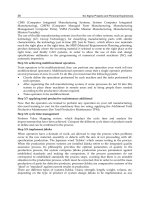
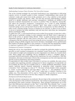
The analysis for the data from Table 6 was run with a main effect full model. This model is
saturated; therefore the two main effects with the smallest Sum of Squares were left out
from the model. This is that Machine and Cycle time do not affect the electrical Performance.
The analysis for the reduced model is presented in Figure 4. It can be observed that the
Pressure and the Tooling Height are significant with p-values of 0.001, and 0.020,
respectively.

Successful Projects from the Application of Six Sigma Methodology
97

Pressure (psi)

Tooling
Height (in)

Cycle Time
(milliseconds)

Machine

% Acceptable
95 0.060 6000 1 0.9951
95 0.070 7000 2 0.9838
95 0.080 8000 3 0.9908
100 0.060 7000 3 0.9852
100 0.070 8000 1 0.9713
100 0.080 6000 2 0.986
110 0.060 8000 2 0.9639
110 0.070 6000 3 0.9585
110 0.080 7000 1 0.9658
Table 6. Results of Runs in Grit Blast


Fig. 4. ANOVA for the Reduced Model for the Grit Blast Parameters

Mean of % A ccept able
11010095
0.99
0.98
0.97

0.96
0.080.070.06
800070006000
0.99
0.98
0.97
0.96
321
Pressure (psi) Tooling Height (in)
Cy c le T im e ( m illi se c ) Machine
Main Effects Plot (fitted means) for % Acceptable

Fig. 5. Chart in Benchmarks Main Effects of Grit Blast

Six Sigma Projects and Personal Experiences
98
The Figure 5 shows the main effects plot for all four factors, which confirm that only
Pressure, Tooling Height and Cycle Time are affecting the quality characteristic. Figure 6
shows that normality and constant variance are satisfied.

Residual
Percent
0.00500.00250.0000-0.0025-0.0050
99
90
50
10
1
N9
AD 0.408

P-Value 0.271
Fitted Value
Residual
0.990.980.970.96
0.0030
0.0015
0.0000
-0.0015
-0.0030
Residual
Frequency
0.0020.0010.000-0.001-0.002-0.003
3
2
1
0
Observation Order
Residual
987654321
0.0030
0.0015
0.0000
-0.0015
-0.0030
Normal Pro bability Plot Residuals Versus the Fitt ed Values
Histogram of the Residuals Residuals Versus the Order of the Dat
a
Residual Plots for % Acceptable

Fig. 6. Residual Plots for the Acceptable Fraction.

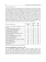
Finally, with the intention of determining whether there is a difference in performance of
four shifts, a test analysis of variance and equality of means was performed. The Table 7
shows that there is a difference between at least one of the shifts, since the p-value is less or
equal to 0.0001. The above analysis indicates that all four shifts are not working with the
same average efficiency. For some reason shift A presents a better performance in electrical
test. Also it can be observed that shift D has the lowest performance. With the intention of
confirm this behaviour; a test of equal variances was conducted. It was observed that the
shift A shows less variation than the rest of the shifts, see Figure 7. This helps to analyze best
practices and standardized shift A in the other three shifts.
Once it was identified the factors that significantly affect the response variable being
analyzed, the next step was to identify possible solutions, implement them and verify that
the improvement is similar to the expected by the experimental designs. According to the
results obtained, corrective measures were applied for the improvement of the significant
variables.
With regard to the inefficient identification of flaws in the failure analysis, and given that
33% of electrical faults analyzed in the laboratory could not be identified with the test
equipment that was used. Then, a micromanipulator was purchased. It allows the test of
circuits from its initial stage. Furthermore, it is planned the purchase of another equipment
different than the currently used in the laboratory of the matrix plant at Lexington. This
equipment decomposes the different layers of semiconductor and determines the other
particles that are mixed in them. These two equipments will allow the determination of the

Successful Projects from the Application of Six Sigma Methodology
99
particles mixed in the semiconductor and clarify if they are actually causing the electrical
fault, the type of particle and the amount of energy needed to disintegrate.

One-way ANOVA: Shifts A, B, C y D
Source DF SS MS F P
Factor 3 13.672

4.557 9.23 0.000
Error 124 61.221

0.494
Total 127 74.894
S = 0.7027 R-Sq = 18.26% R-Sq(adj) = 16.28%
Individual 95% CIs For Mean Based on Pooled StDev
Level

N

Mean

StDev

+ + + +
A 32

3.0283

0.4350

( * )
B 32

3.6078

0.6289

( * )
C 32

3.5256

0.8261

( * )
D 32

3.9418

0.8412

( * )
+ + + +
2.80 3.20 3.60 4.00
Pooled StDev = 0.7027
Table 7. ANOVA Difference between Shifts


Fig. 7. Equality of Variance Test for the Shifts
About the percentage of defective electrical switches with different thicknesses of Procoat (0,
14, 30 and 42 microns). The use of Procoat will continue because the layer has a positive
effect on the electrical performance of the circuit. However, because the results also showed
that increasing the thickness of the layer from 14 to 42 microns, does not reduce the level of
electrical defects. The thickness will be maintained at 14 microns.
For the drilling pressure in the equipment, lower levels are better and for the improvement
of the electrical performance without affecting other quality characteristics, such as the
dimensions of width and length of the track. It was determined that the best level for the

D
C
B
A
1.21.00.80.60.40.2
SHIFT
95% Bonferroni Confidence Intervals for StDevs
Test Statistic 15.21
P-Value 0.002
Test Statistic 3.68
P-Value 0.014
Bartlett's Test
Levene's Test
Test for Equal Variances for Shifts

Six Sigma Projects and Personal Experiences
100
pressure would be 95 psi. With respect to the height of the drill, since it significantly affects
the electrical performance and this is better when the tool is kept at 0.60 or 0.80 inches on the
semiconductor. For purposes of standardization, the tool will remain fixed at a height of 0.60
inches.
In relation to the cycle time, it showed to be a source of conflict between two quality
characteristics (size of the track and percentage of electrical failures). Although it is a factor
with a relatively low contribution to the variation of the variable analyzed. Several
experiments were run with the parameters that would meet the other characteristic of
quality. Figure 5 shows the main effect. For the variable electrical performance, a factor
behavior of the type smaller is better was introduced. While for the other variable output
capacity of the process, a higher is better behavior was selected and for that reason, it was
determined that this factor would be in a range from 7,000 to 8,000 milliseconds.
Finally, with respect to the difference between the four-shift operations and electrical

performance, results indicate that the “A” shift had better electrical performance, with the
intention of standardization and reduction of the differences, a list of best practices was
developed and a training program for all shifts was implemented. In this stage is
recommended an assessment of the benefits of the project (Impact Assessment of
Improvement). Once implemented the proposed solutions, a random sample size 200 was
taken from one week work inventory product and for all shifts. This sample was compared
to a sample size 200 processed in previous weeks. Noticeable advantages were found in the
average level of defects, as well as the dispersion of the data. Additionally, the results of the
tested hypotheses to determine if the proposed changes reduced the percentage defective.
Electrical test indicate that if there is a difference between the two populations.


Fig. 8. Box Plots for the Nonconforming Fractions of Before and After
In Figure 8, Box diagrams are shown for the percentage of defects in the two populations. It
is noted that the percentages of defects tend to be lower while maintaining the parameters of
the equipment within the tolerances previously established as the mean before
implementation is 3.20%, against 1.32% after implementation. The test for equality of
variances shows that in addition to a mean difference there is a reduction in the variation of
the data as shown in see Figure 9. Figure 10 shows a comparison of the distribution of
defects before and after implementation. It can be seen that the defect called "Aluminum
oxide residue" was considerably reduced by over 50%.
AfterBefore
8
6
4
2
0
% Defe cts

After 1.267 0.400

Before 3.32 1.39
Mean StDev

Successful Projects from the Application of Six Sigma Methodology
101

Fig. 9. Test of Equality of Variances for the Nonconforming Fractions of Before and After
Control: In order to achieve stable maintain the process, identified the controls to maintain
the pressure, height of the tool and cycle time within the limits set on the computer Grit
Blast and test electrical equipment. Identification of Controls for KPIV's: Because these three
parameters had been covered by the machine operator to offset some equipment failures
such as leaks or increasing the cycle time. It was necessary to place devices that will facilitate
the process control in preventing any possible change in the parameters.


Fig. 10. Distribution of Defects Before and After
Additionally, to help keep the machine operating within the parameters established without
difficulty, it was essential to modify the plan of preventative maintenance of equipment.
Due to the current control mechanisms are easily accessible to the operator; it was
determined to improve those controls to ensure the stability of the equipment and process.
All of this coupled with an improvement in preventative maintenance of the equipment.
Based on the information generated with the assessment of the assumptions above, it
generated an action plan which resulted in a reduction in the percentage of electrical failures
After
Befo re
1.501.251.000.750.50
95% Bonferroni Confidence Intervals for StDevs
After
Befo re
86420

% Defects
Test Statistic 12.08
P-Value 0.000
Test Statistic 134.42
P-Value 0.000
F-Tes t
Levene's Test
Test for Equal Variances for Before, After
% of Defects
1.3
2
0.61
3
0.50
6
0.23
3
0.15
5
0.37
2
0.44
8
0.075
5
0.25
6
0.01
1
0.31

8
0.21
0
0.2
0.4
0.6
0.8
1
1.2
1.4
Residuals
A1203
Indetects
defects
Scratch Error
Tester
Broke Others
Defects
%
Before
After

Six Sigma Projects and Personal Experiences
102
in general. As well as a reduction in the defect called "Short but residue of aluminum oxide".
Table 8 shows a comparison of the nonconforming fraction, PPM’s and Sigma levels of
before and after implementation.

% Defects Sigma Level PPM’s
Base Line 3.20 3.35 31982

Goal 1.60 3.64 16000
Evaluation 1.32 3.72 13194
Table 8. Comparison of Before and After
Conclusion: The implementation of this project has been considered to be a success. Since,
the critical factor for the process were found and controlled to prevent defects. Therefore the
control plan was updated and new operating conditions for the production process. The
based line of the project was 3.35 sigma level and the gain 0.37 of sigma. Which represent
the elimination of 1.88% of nonconforming units or 18,788 PPMs. Also, the maintenance
preventive program was modified to achieve the goal stated at the beginning of the project.
It is important to mention that the organization management was very supportive and
encouraging with the project team. The Six sigma implementation can be helpful in
reducing the nonconforming units or improving the organization quality and personal
development.
4. Capability improvement for a speaker assembly process
A Six Sigma study that was applied in a company which produces car speakers is presented.
The company received many frequent customer complaints in relation to the subassembly of
the pair coil-diaphragm shown in Figure 11. This subassembly is critical to the speaker
quality because the height of the pair coil-diaphragm must be controlled to assure adequate
functioning of the product. Production and quality personnel considered the height was not
being properly controlled. This variable constitutes a high potential risk of producing
inadequate speakers with friction on the bottom of the plate and/or distortion in the sound.
Workers also felt there had been a lack of quality control in the design and manufacture of
the tooling used in the production of this subassembly. The Production Department as well
as top management decided to solve the problems given the cost of rework overtime pay
and scrap which added up to $38,811 U.S. dollars in the last twelve months. Improvement of
the coil-diaphragm subassembly process is presented here, explaining how the height
between such components is a critical factor for customers. This indicates a lack of quality
control.
Define: For deployment of the Project, a cross functional project team was integrated with
Quality, Maintenance, Engineering, and Production personnel. The person in charge of the

project trained the team. In the first phase, the multifunctional 6σ team made a precise
description of the problem. This involved collecting the subassemblies with problems such as
drawings, specifications, and failure modes analyses. Figure 11 shows the speaker parts and
the coil-diaphragm subassembly. The subassembly was made in an indexer machine of six
stations. The purpose of this project was to reduce quality defects; specifically, to produce
adequate subassemblies of the coil-diaphragm. Besides, the output pieces must be delivered
within the specifications established by the customer. The objective was to reduce process
variation with the Six Sigma methodology and thus attain a Cpk ≥1.67 to control the tooling.

Successful Projects from the Application of Six Sigma Methodology
103

Fig. 11. Speaker Explosion Drawing
Then, the critical characteristics were established and documented based on their frequency
of occurrence. Figure 12 shows the five critical defects found during a nine month period. It
can be seen that height of the coil-diaphragm out of specifications is the most critical
characteristics of the speaker, since it contributes 64.3% of the total of the nonconforming
units. The second highest contributing defect is the distortion with 22.4%. These two types
of nonconforming speakers accumulate a total of 86.8%. By examining Figure 10, the Pareto
chart, it was determined that the critical characteristic is the height coil-diaphragm. The
project began with the purpose of implementing an initial control system for the pair coil-
diaphragm. Then, the Process Mapping was made and indicated that only 33.2% of the
activities add value to parts.

Count
Percent
Defect
Count
5.7 4.5 3.0
Cum % 64.3 86.8 92.5 97.0 100.0

4679 1632 415 328 219
Percent 64.3 22.4
O
t
h
e
r
W
e
i
g
h
t

o
f

A
d
h
e
s
i
v
e
C
u
r
e

T
i
m
e

A
d
h
e
s
i
v
e
D
i
s
t
o
r
t
i
o
n
H
e
i
g
h
t

C
o
i
l
-
D
i
a
p
h
r
a
g
m
8000
7000
6000
5000
4000
3000
2000
1000
0
100
80
60
40
20
0
Pareto Chart of Defect

Fig. 12. Pareto Diagram for Types of Defects
Also the cause and effect Matrix was developed and is shown in Table 9. It indicates that
tooling is the main factor that explains the dispersion in the distance that separates coil and

Six Sigma Projects and Personal Experiences
104
diaphragm. At this point, there was sufficient evidence that points out the main problem
was that the tooling caused variation of the height of the coil diaphragm.
Measurement: Gauge R&R and process capability index Cpk studies were made to evaluate
the capability of the measuring system and the production process. Simultaneously, samples
of the response variables were taken and measured. Several causes of error found in the
measurements were: the measuring instrument, the operator of the instrument and the
inspection method.


Level of Effect


Step
Number

1 NO
EFFECT


4
MODERATE
EFFECT
Present

Functionality

Appearance

Adhesion Total
9 STRONG EFFECT

Factor in
Process

1 Tooling 9 9 9 9 342
2 Diaphragm
dimension
9 9 4 9 302
3 Weight of
adhesive
9 9 4 9 302
4 Weight of
accelerator
9 9 4 9 302
5 Diameter of
coil
9 9 9 4 292
6 Cure time 9 9 4 4 252
7 Injection devise

9 9 4 4 252
8 Air pressure 9 9 4 4 252
9 Wrong

material
9 9 4 4 252
10 Broken
material
9 4 4 4 202
11 Personal
training
9 9 1 1 198
12 Manual
adjustment
1 4 4 4 122
13 Production
Standard
1 9 1 1 118
14 Air 1 1 1 1 38
Table 9. Cause and Effect Matrix for the Height of Coil-Diaphragm
To correct and eliminate errors in the measurement system, the supervisor issued a directive
procedure stating that the equipment had to be calibrated to make it suitable for use and for
making measurements. Appraisers were trained in the correct use and readings of the
measurement equipment. The first topic covered was measurement of the dimension from

Successful Projects from the Application of Six Sigma Methodology
105
the coil to the diaphragm, observing the specifications. The next task was evaluation of the
measurement system, which was done through an R&R study as indicated in (AIAG, 2002).
The study was performed with three appraisers, a size-ten sample and three readings by
appraiser. An optical comparative measuring device was used. In data analysis, the
measurement error is calculated and expressed as a percentage with respect to the
amplitude of total variation and tolerance. Calculation of the combined variation
(Repeatability and reproducibility) or error of measurement (EM): P/T =

Precision/Tolerance, where 10% or less = Excellent Process, 11% to 20% = Acceptable, 21%
to 30% = Marginally Acceptable. More than 30% = Unacceptable Measurement Process and
must be corrected.
Since the result of the Total Gage R&R variation study was 9.47%, the process was
considered acceptable. The measuring system was deemed suitable for this measurement.
Likewise, the measuring device and the appraiser ability were considered adequate given
that the results for repeatability and reproducibility variation were 8.9% and 3.25%,
respectively. Table 10 shows the Minitab© output.
The next step was to estimate the Process capability index Cpk. Table 11 shows the
observations that were made as to the heights of the coil-diaphragm. The result of the index
Cpk study was 0.35. Since the recommended value must be greater than 1, 1.33 is acceptable
and 1.67 or greater is ideal. The process then was not acceptable. Figure 13 shows the output
of the Minitab© Cpk study. One can see there was a shift to the LSL and a large dispersion.
Clearly, the process was not adequate because of the variation in heights and the shift to the
LSL. A 22.72% of the production is expected to be nonconforming parts.

Source StdDev(SD)

Study Var (5.15*SD)

%Study Var(%SV)
Total Gage R&R

0.022129 0.11397 9.47
Repeatability 0.020787 0.10705 8.90
Reproducibility 0.007589 0.03908 3.25
C2 0.007589 0.03908 3.25
Part-To-Part 0.232557 1.19767 99.55
Total Variation

0.233608 1.20308 100.00
Number of Distinct Categories = 15
Table 10. Calculations of R&R with Minitab©

Height/
Measurement
Sample/Hour
1 2 3 4 5 6 7 8 9 10 11
1 4.72 4.88 5.15 4.75 4.42 4.76 5.14 5 4.88 4.66 4.75
2 4.67 4.9 5 4.4 4.81 4.81 4.78 4.8 5 4.58 4.88
Table 11. Heights of Coil-Diaphragm before the Six Sigma Project
Verification of the data normality is important in estimating the Cpk, which was done in
Minitab with the Anderson-Darling (AD) statistic. Stephens (1974) found the AD test to be
one of the best Empirical distribution function statistics for detecting most departures from
normality, and can be use for n greater or equal to 5. Figure 14 shows the Anderson-Darling
test with a p-value of 0.51. Since the p-value was greater than 0.05 (α=0.05), the null
hypothesis was not rejected. Therefore, the data did not provide enough evidence to say that
the process variable was not normally distributed. As a result, the capability study was valid
since the response variable was normally distributed.

Six Sigma Projects and Personal Experiences
106
5.65.45.25.04.84.64.4
LSL USL
Process Data
Sample N 22
StDev(Within) 0.199818
StDev (O v erall) 0.196192
LS L 4.6
Target *

USL 5.6
Sample Mean 4.80636
Potential (Within) C apability
C C pk 0.83
O v erall C apability
Pp 0.85
PPL 0.35
PPU 1.35
Ppk
Cp
0.35
Cpm *
0.83
CPL 0.34
CPU 1.32
Cpk 0.34
Observed Performance
PPM < LSL 136363.64
PPM > USL 0.00
PPM Total 136363.64
Exp. Within Performance
PPM < LSL 150858.54
PPM > U S L 35.67
PPM Total 150894.21
Exp. O verall P erformance
PPM < LSL 146435.73
PPM > USL 26.14
PPM Total 146461.87
Within
Overall

Process Capability of Height Coil-Diaphragm

Fig. 13. Estimation of the Cpk Index for a Sample of Coil-Diaphragm Subassemblies

Height Coil_diaphra gm
Percent
5.35.25.15.04.94.84.74.64.54.4
99
95
90
80
70
60
50
40
30
20
10
5
1
Mean
0.510
4.806
StDev 0.1939
N22
A D 0.321
P-Value
Probability Plot of Height Coil_diaphragm
Nor mal

Fig. 14. Normality Test of the Coil-Diaphragm Heights
Analysis: The main purpose of this phase was to identify and evaluate the causes of
variation. With the Cause and Effect Matrix, the possible causes were identified. Afterward,
the Six Sigma Team selected those which, according to the team’s consensus, criteria and
experience, constituted the most important factors. With the aim of determining the main
root-causes that affected the response variable, a diagram of cause and effect (Ishikawa
diagram) was prepared in a brainstorm session where the factors that influenced the height
between the coil and the diaphragm were selected. The causes were statistically analyzed,
and the tooling was found to have had a moderate effect in the critical dimensions. The
tooling effect had the largest component of variation. Several causes were found: first, the
tools did not fulfill the requirements, and their design and manufacture were left to the
supplier; also, the plant had no participation in designing the tools; second, the weight of

Successful Projects from the Application of Six Sigma Methodology
107
the adhesives and the accelerator were not properly controlled. Since the tools were not
adequate given that some variation was discovered in the amounts delivered, this had an
impact on the height.
The tooling was analyzed to check whether the dimensions had affected the height between
the coil and the diaphragm. The regression analysis was made to verify the hypothesis that
the dimensions of the tooling do not affect the height between the coil and the diaphragm.
The First two test procedures used to verify the above hypothesis were the regression
analysis and the one-way ANOVA. The results of both procedures were discarded because
the basic assumptions about normality and homogeneity in the variances were not satisfied.
Then the Kruskal-Wallis test was carried out to verify the hypothesis. The response variable
was the Height of the Coil-Diaphragm and the factor was the Tooling height. Table 12
illustrates the results
Figure 15 shows the results of Kruskal Wallis analysis with a p-value less than 0.001. Then
the decision is to reject the null hypothesis. Consequently, it is concluded that the data
provide sufficient evidence to say that the height of the tooling affects the height of

subassembly coil- diaphragm.


Tooling Height

Coil-Diaphragm Height (in mm)
Levels 1 2 3 4 5 6 Mean
1 4.78 4.70

4.75

4.70

4.75

4.78

4.76

4.74
2 4.88 4.81

4.83

4.85

4.87

4.81

4.81

4.83
3 4.90 4.88

4.91

4.95

4.94

4.92

4.93

4.92
4 5.00 5.10

5.20

4.98

4.98

5.31

4.97

5.09
5 5.10 5.12

5.14

5.23

5.20

5.19

5.31

5.19
6 5.30 5.40

5.55

5.38

4.97

4.99

5.39

5.28
Table 12. Results of Tooling Height vs. Coil-Diaphragm Height


Fig. 15. Result of Kruskal Wallis Test
In addition, the thickness of the diaphragm was analyzed. A short term sample of pieces of

diaphragms were randomly selected from an incoming lot, and measured to check the
capability of the material used in the manufacturing. This analysis was conducted because

Six Sigma Projects and Personal Experiences
108
when the thickness of the diaphragm could be out of specification and the height coil-
diaphragm could be influenced. The diaphragm specifications must have a thickness
between 0.28 ± 0.03 mm for a certain part number. The material used in the subassembly is
capable because the measurements were within specifications and had a Cpk of 1.48. Which
is acceptable because was greater than 1.33. Also, the weight of adhesive was analyzed,
thus, another short term sample of 36 deliveries were weighted. The weight of the glue must
be within 0.08 and 0.12 grams. The operation of delivering the adhesives in the subassembly
is capable because the Cpk was equal to 3.87, which greater than 1.67 and acceptable. The
weights of the adhesive appear to be normal. Regarding the accelerator weight, 36
measurements were made on this operation, whose specifications are from 0.0009 to 0.0013
grams. Also, the data about weights of the accelerator indicates a Cpk of 1.67. Therefore, this
process was complying with the specifications of the customer.
Finally, the Multi-Vari analysis allowed the determination of possible causes involved in the
height variation. To do the Multi-Vari chart, a long term random sample of size 48 was
selected, stratifying by diaphragm batch, speaker type and shift. The main causes of
variation seem to be the batch raw material (diaphragm and coil) used, and the second work
shift in which the operators had not been properly trained. See Figure 16. Two different lots
of coil and the two shifts were included in the statistical analysis to verify whether raw
material and shifts were affecting the quality characteristic. The results of multivariate
analysis indicated that these factors did not influence significantly the subassembly height.

Speaker Type
Diaphragm Thickness
21
5.180

5.175
5.170
5.165
21
1 2
Diaphragma
Batch
1
2
Multi-Vari Chart for Diaphragm Thickness by Diaphragma Batch - Shift
Panel variable: Shift

Fig. 16. Multi-Vari chart for Height by Batch, Speaker Type and Shift.
Improvement: In the previous phase, one of the causes of variation on the Height of Coil-
Diaphragm was found to be the Tooling height. The tooling height decreases due to the
usage and wearing out. The phase began with new drawings of the tooling subassembly coil
and diaphragm, and the verification and classification of drawings and tooling, respectively.
The required high-store tools (maximum and minimum) supplemented this as well. Tooling
drawings were developed for the production of the subassemblies coil-diaphragm, the coil-
diaphragm subassemblies, controlling the dimensions carefully according to work
instructions. No importance had been previously given to the tools design, drawings and
production.

Successful Projects from the Application of Six Sigma Methodology
109
After all the improvements were carried out, a sample of thirty-six pieces was drawn to
validate the tooling correction actions by estimating the Cpk. The normality test was
performed and the conclusion was that the data is not normally distributed. Then, Box-Cox
transformation was applied to the reading to estimate the process capability. Figure 17
shows the substantial improvement made in the control of the heights variation. The study

gave a Cpk of 2.69; which is greater than 1.67. This is recommended for the release of
equipment and tooling.
Control: This investigation in addition to the support of management and the team all
strengthened the engineering section and led to very good results. A supervisor currently
performs quality measurements of the tooling for control. Such a tooling appraisal was not
carried out as part of a system in the past, but now it is part of the manufacturing process.
This change allowed an improvement through the control of drawings and tooling as well
as by measuring the tooling before use in the manufacture of samples and their release.

54004950450040503600315027002250
LS L* Target* USL*
transformed data
Process Data
Sample N 36
StDev (Within) 0.0560084
StDev (O v erall) 0.0567162
A fter Transformation
LSL* 2059.63
Target*
LS L
3450.25
U SL* 5507.32
Sample M ean* 3695.9
StDev (Within)* 199.021
StDev (O v erall)* 203.1
4.6
Target 5.1
USL 5.6
Sample M ean 5.16944
P otential (Within) C apability

CCpk 2.33
O v erall C apability
Pp 2.83
PPL 2.69
PPU 2.97
Ppk
Cp
2.69
Cpm 1.45
2.89
CPL 2.74
CPU 3.03
Cpk 2.74
O bserv ed P erform ance
PPM < LSL 0.00
PPM > USL 0.00
PPM Total 0.00
Exp. Within Performance
PPM < LSL* 0.00
PPM > USL* 0.00
PPM Total 0.00
Exp. Overall Performance
PPM < LSL* 0.00
PPM > USL* 0.00
PPM Total 0.00
Within
Overall
Process Capability of C1
Using Box-Cox Transformation With Lambda = 5

Fig. 17. Estimation of Cpk for Height Coil-Diaphragm with Control in the Tooling
A management work instruction was mandatory to control the production of manufacturing
tooling for subassemblies. The requirement was fulfilled through the high-quality system
ISO / TS 16949 under the name of "Design Tools”. Furthermore, management began to
standardize work for all devices used in the company. The work instruction "Inspection of
Critical Tooling for the Assembly of Horns” was issued and applies to all the tooling
mentioned in the instruction. Design of the tooling was documented in required format that
contains the evidence for the revision of the tooling. Confirmatory tests were conducted to
validate the findings in this project, and follow-up runs to be monitored with a control chart
were established.
Conclusion: At the beginning of this project, the production process was found to be
inadequate because of the large variation: Cpk´s within 0.35, as can be seen in Figure 13.
Implementing the Six Sigma methodology has resulted in significant benefits, such as no
more re-tooling or rework, no more scrap, and valuable time saving, which illustrates part
of the positive impact attained, the process gave a Cpk of 2.69, as shown in Figure 17.
Furthermore, this project solved the problem of clearance between the coil and the
diaphragm through the successful implementation of Six Sigma. The estimated savings per
year with the subassembly is $31,048 U.S. dollars. The conclusion of this initial project has
helped establish the objective to go forward with another Six Sigma implantation, in this
case to reduce distortion in the sound of the horn.

Six Sigma Projects and Personal Experiences
110
5. Improvement of binder manufacturing process
In process of folders, a family of framed presentation folders is manufactured. The design
has a bag for placing business cards. The first thing that took place in this project was to
define the customer requirements:
1. Critical to Quality: Folders without damage and without Flash.
2. Critical for Fill Rate: Orders delivered on time to the distribution centers and orders
delivered on time to customers.

3. Critical for Cost: Less waste of materials and scrap.
Define: The problem is that the flash resulting in the sealing operation of business cards,
damages the subsequent folders rivet operation, reducing the quality and increasing the
levels of scrap. Figure 18 shows the sample of the location and the business card bag. The
Figure 19 shows the distribution of plant where the problem appears.

Fig. 18. Folder and Business Card Holder


Fig. 19. Layout of the machines Rotary Table 5& 6