Supply Chain Management Part 7 docx

A Cost-based Model for Risk Management in RFID-Enabled Supply Chain Applications
231
The value of each row is either 1,2,3, 4 or 5 and represent the rank (shown in Table 27). Since
smaller rank value is more preferable than higher rank value. Table 28 indicates that each
criterion has a different range. For instance, the range for cost is in indicated in dollars in
contrast to that for acceptance which is indicated in rank. It is not viable to the sum of the
values of the different multiple criteria does not deliver a valid result. We need to transform
the score of each factor according to its range value so that all factors have comparative
ranges.

Criterias|
Techniques
EPC
Design
Tags
Design
Lightweight
Protocol
Lightweight
ECC
Steganography Range
Acceptance
3 4 1 2 5 1-5
Cost
1.5 5 0.5 1 2
$0.5 -
$5.00
Security
1 0.8 0.3 0.6 0.5 0.3-1
Complexity
2 1 3 4 5 1-5

Sum
7.5 10.8 4.8 7.6 12.5 43.2
Normalized
Score
20.66% 18.75% 22.22% 20.60% 17.77% 100%
Table 28. Evaluation based on range scores of Tag’s authencity Techniques for Various
Supply Chain Criterias
We transform the score value of each factor to have the same range value of 0 to 1. A
formula based on the simple geometry of a line segment is used to linearly convert the score
of each factor from table 28 to table 30 to a single shared range.
new score =
(original score – olb) + nlb (16)
Each factor has different importance weightings based on its organisation’s priorities. Since
the weighting is a subjective value, the result changes with changes to the factors’
weightings. Table 29 displays an example of organisation ‘A ‘are weighting priorities in
selecting their most appropriate tag authentication methodology.

Acceptance Cost Security Complexity Sum
Importance
Level
20 40 30 10 100
Importance
Weight
20.0% 40.0% 30.0% 10.0% 100.0%
Table 29. Supply Chain Criteria’s Weight of Importance
Table 30 shows the end result of normalizing the weighting of each factor, demonstrating
the opportunity for an organization to compare different based factors based on a
normalised range where individual factors are weighed according to the organization’s
personal requirements and needs. We are able to demonstrate that, for a organisation ‘A’
that emphasizes cost factors over security factors, a lightweight ECC would be the most

appropriate technique for securing their low cost tags. This result contraindicates the
prediction that lightweight ECC might be the preferred way in the future for securing low
Supply Chain Management
232
cost tags. This prediction is based on the fact that lightweight ECC uses only 64K of RFID
tag storage and provides strong authenticity comparable to that of any other lightweight
public key infrastructure.

Criterias|
Techniques
Weights EPC
Design
Tags
Design
Light-
weight
Protocol
Lightweight
ECC
Stegano-
graphy
Acceptance
20.0% -0.100 -0.100 -0.200 -0.150 0.200
Cost
40.0% 0.011 -0.067 0.033 0.022 -0.033
Security
30.0% -0.071 -0.043 0.029 -0.014 -0.029
Complexity
10.0% 0.150 0.200 0.100 0.050 -0.200
Sum

100.0% -0.010 -0.010 -0.038 -0.092 -0.062 -0.212
Normalized
Score

4.9% 4.5% 18.0% 43.4% 0.292134831 100.0%
Table 30. Supply Chain Criteria’s and Techniques Weighted scores
6. Applicability discussions
In this section, we analyze how well MCDM quantified costs associated with cloning and
fraud attacks. In the first part we discuss on the MCDM quantified cost result for cloning
attack. The second part discusses the cost results obtained for fraud attacks, and for SA tests
and authentication exercises. Finally, we analyze the validity of using cost sensitive and cost
insensitive models for costing purposes.
6.1 RFID Tag cloning attack
Based on the result obtained from the MCDM approach, a ‘man in the middle’ attack has the
highest Damage Cost of all attacks. This shows that a high Damage Cost is not associated
with highly complex attacks (e.g. ‘physical’ attacks) or with easy attacks (e.g. ‘skimming’
attacks), but with specific techniques used in and means of the attack taking place. Although
unavailability and disclosure Damage associated with ‘man in the middle’ attacks has an
high risk impact on the occurrence of future cloning and fraud attacks, simpler attacks have
a much lower Response Cost.
A comparison of consequential costs (the summation of Damage and Response Costs)
indicate that both ‘eavesdropping’ and MIM attacks have a higher consequential cost than
other attacks. Time factors are used in the ranking system, correspondent to the level of
complexity in detecting and responding to the attack, to calculate Operational Costs
associated with an IDS handling a cloning or fraud attack. MCDM criteria include extracted
test features from raw RFID streams. There are four different levels of extracting test
features. Our results indicate that highest rank extracted test features are from an
interconnected supply chain partner’s organisation within an EPCglobal service, due to the
difficulty in obtaining shared computing resources between different partners and
establishing various EDI services among them.

Cumulative Cost calculations indicate the association of the highest cumulative Operational
Costs with ‘man in the middle’ attacks and of the lowest costs with ‘skimming’ attacks.
Based on this information, we conclude that ‘man in the middle’ cloning attacks cause the
A Cost-based Model for Risk Management in RFID-Enabled Supply Chain Applications
233
greatest overall losses in terms of money, time and computing resources. This result implies
that measures to prevent ‘man in the middle ‘cloning attacks in a supply chain management
is likely to minimise the impact of counterfeiting on an organisation.
The prevention measures that could be taken in eliminating MIM attacks include: 1) refresh
the tag secret key immediately after a reader has been authenticated; 2) maintain tag output
changes, as this minimises opportunities for replay attacks and the related risk of a faked
tag; 3) keep the number of communication rounds and operation stages minimal to avoid
redundant operations; maintain scalability and eliminate the risk of ‘man in the middle; and
4) design the coordinating global item tracking server to include a timely tracking system
that maintains freshness necessary due to the randomness of keys used in inter-
organisational item-tracking activities.
6.2 RFID tag fraud, SA testing and authentication techniques
The main differences between fraud and cloning attacks in regards to the similar Damage;
response; and Operational Cost types, are based on the criteria factors used in applying a
MCDM tool to calculate these costs. Fraud attack costs are associated with the progress of
the attack rather than with the type of attack that contributed to it. This is due to the fact that
a fraud attack occurs only after a tag has successfully been cloned after one or more
previous attacks. The progress of a fraud attack is closely associated with inconsistency of
tag count, related to the travel of tags to unauthorised locations:; the need for a higher
bandwidth for fraud detection in unauthorised locations; and inconsistencies between travel
timeframes associated with illegal tags. Similar criteria factors are used to calculate costs
associated with SA testing.
In a comparison of CCost for cloning and fraud attacks, the latter attack type has
significantly lower associated CCost. This is due to the fact that fraud attacks are a part of
cloning attack SA test costs are calculated using only Damage Cost, as SAs do not have

malicious intentions towards the system and are able to use the system only after their
system authentication, which is transparent during system audit procedures, classified as
usage by a legal and authorised user.
Biometric authentication methods are the most secure and suitable method for use by
supply chain partners in supply chain management, as indicated by the AHP tool. The SHA
algorithm can be used to create a ‘fingerprint’ for the public key of this biometric
application. Tag authentication methods that minimise storage needs and use minimal key
bits are preferred, such as lightweight public cryptography (e.g. ECC and lightweight
protocol).
6.3 Cost sensitive vs. Cost insensitive
We have extended the MCDM tool for evaluating CCost (Damage and Response Costs)
calculations in our cost model. The aim for calculating both Damage and Response Costs is
the evaluation the cost impact of a cost sensitive vs. that of a cost insensitive cost model. The
difference between the cost impact of a cost sensitive and cost insensitive model is that a
cost sensitive model initiates an SA alert only if DCost ≥ RCost and if it corresponds to the
cost model. Cost insensitive methods, in contrast, respond to every predicted intrusion and
are demonstrated by current brute-force approaches to intrusion detection.
Estimation of losses indicates that it could be reduced by up to 73% if a cost sensitive model
is used in a system.
Supply Chain Management
234
This impressive result is obtained using quantified cost for counterfeiting; and indicate that
to optimally curb both cloning and fraud attacks, it is necessary to aim to minimise false
negative in a system rather than to optimise accuracy of detection and elimination of false
positives. The underlying principle for every business model should remain to minimise
financial losses without compromising system security or product quality.
In addition our RFID cost model also included testing cost operated on the detector system
by supply chain employee; the system administrator. The result display that testing cost
only takes up less than 10% for every misclassifications cost reported. As the role of testing
indicates the relevance of IDS and boost the accuracy of the dataset rules, the component of

testing should never be compromised on the ground of losses in dollar.
The result also indicates the significance of calculating both misclassification and testing cost
in any cost model.
7. Conclusions and future research
In this chapter, we have proposed cost-based approach using MCDM tool to quantify cost
when curbing counterfeiting in RFID-enabled SCM. We have extended this tool to analyze
the different authentication approaches, including for tag authentication, which can be used
by system administrators. We have shown that the MCDM approach could be used for
implementing a practical cost-sensitive model, as validated by our analytical results. We
contend that the definitions of damage; response; and operational costs are complex,
especially when applying theoretical attack criticality and progress attack in determining
cloning and fraud costs. Our future work will focus on the implementation of our cost
model and on development of robust RFID tag detectors for cloning and fraud attacks. We
will use the cost model to estimate costs to predict total financial losses related to RFID tag
cloning and fraud.
8. Acknowledgements
This work is partially sponsored by University Sains Malaysia (USM) and the NSFC JST
Major International (Regional) Joint Research Project of China under Grant No. 60720106001.
9. References
S. Bono et al.: Security Analaysis of a Cryptographically-Enabled RFID Device. In P.
McDaniel, ed., USENIX Security ’05, pp. 1-16. 2005.
E.Y. Choi, D.H. Lee and J.I. Lim: Anti-cloning protocol suitable to EPCglobal Class-1
Generation-2 RFID systems, Computer Standards and Interfaces 31 (6) (2009), pp.
1124–1130.
L. Bolotnyy, G. Robins: Physically Unclonable Function-Based Security and Privacy in RFID
Systems, percom, pp.211-220, Fifth IEEE International Conference on Pervasive
Computing and Communications (PerCom'07), 2007
D.N. Duc, Park, J., Lee, H., Kim, K.: Enhancing Security of EPCglobal GEN-2 RFID Tag
against Traceability and Cloning. In: Symposium on Cryptography and Information
Security, Hiroshima, Japan (January 17-20, 2006)

T. Dimitriou., “A Lightweight RFID Protocol to protect against Traceability and Cloning
attacks” in Security and Privacy for Emerging Areas in Communications Networks, 2005.
A Cost-based Model for Risk Management in RFID-Enabled Supply Chain Applications
235
SecureComm 2005. First International Conference on (05-09 September 2005), pp. 59-
66.
R. Derakhshan, M. E. Orlowska, and X. Li. (2007). RFID data management: Challenges and
opportunities. In: D. W. Engels, IEEE International Conference on RFID 2007. IEEE
International Conference on RFID 2007, Grapevine, Texas, USA, (pp 175-182). 26-28
March, 2008
W .Fan, Lee, W., Stolfo, S., Miller, M.: A multiple model cost sensitive approach for intrusion
detection. In: Proc. Eleventh European Conference of Machine Learning, Barcelona Spain,
pp. 148–156 (2000)
X.Gao Gao, Hao Wang, Jun Shen, Jian Huang, Song, "An Approach to Security and Privacy
of RFID System FOR Supply Chain," Proceedings of the IEEE International
Conference on E-Commerce Technology for Dynamic E-Business (CEC-East’04), pp 164-
168, 2004.
P.T.Hacker: The art and science of decision making: The analytic hierarchy process. In:
Golden, B.L., Wasil, E.A., Harker, P.T. (Eds.), The Analytic Hierarchy Process:
Applications and Studies. Springer, Berlin, pp. 3–36.
A. Juels:RFID security and privacy: a research survey, IEEE Journal on Selected Areas In
Communications, VOL. 24, NO. 2, FEBRUARY 2006, vol. 24, pp. 381-394, 2006.
A. Juels: Strengthening EPC Tags Against Cloning, (M. Jakobsson and R. Poovendran, eds.),
ACM Workshop on Wireless Security (WiSe), pp.67-76. 2005.
S. Kutvonen: Trust management survey, Proccedings of iTrust 2005, number 3477 in LNCS,
pp 77 92 , Springer-Verlag.
W.Lee , Fan, W., Miller, Matt, Stolfo, Sal, Zadok, E.: Toward cost sensitive modeling for
intrusion detection and response. J. Comput. Security 10, pp 5-22 (2002)
W.Lee, Sal Stolfo and Kui Mok, A Data Mining Framework for Building Intrusion Detection
Models. Proceedings of the IEEE Symposium on Security and Privacy, Oakland, CA,

pp. 120-132. 1999.
M.Lehtonen, et.al: Trust and Security in RFID-Based Product Authentication System ,
Systems Journal, IEEE, vol. 1, pp. 129-144, 2007.
M.Lehtonen., Michahelles, F., Fleisch, E.: How to Detect Cloned Tags in a Reliable Way from
Incomplete RFID Traces. In 2009 IEEE International Conference on RFID, Orlando,
Florida, April 27-28, 2009, pp. 257 - 264.
X. Li, J. Liu, Q. Z. Sheng, S. Zeadally, and W. Zhong: TMS-RFID: Temporal Management of
Large-Scale RFID Applications, International Journal of Information Systems Frontiers,
Springer, July 2009,
C. Lin, V.Varadharajan .: A Hybrid Trust Model for Enhancing Security in Distributed
Systems. In: Proceedings of International conference on availability, reliability and
security (ARES 2007), Vienna, pp. 35–42 (2007) ISBN 0-7695-2775-2
C.Lin and V. Varadharajan: Trust Based Risk Management for Distributed System Security -
A New Approach, in Proceedings of the First International Conference on Availability,
Reliability and Security: IEEE Computer Society, pp 6-13 2006.
C.X Ling, V.S Sheng, Q. Yang, "Test Strategies for Cost-Sensitive Decision Trees," IEEE
Transactions on Knowledge and Data Engineering, pp. 1055-1067, August, 2006
U. Lindqvist and E. Jonsson: How to systematically classify computer security intrusions, in
Proceedings of the IEEE Symposium on Research in Security and Privacy, Oakland CA,
May 1997.
Supply Chain Management
236
M. Mahinderjit- Singh and X. Li , "Trust Framework for RFID Tracking in Supply Chain
Management," Proc of The 3rd International Workshop on RFID Technology – Concepts,
Applications, Challenges (IWRT 2009), Milan, Italy, pp 17-26 , 6-7 May 2009.
M. Mahinderjit- Singh and X. Li (2010): Trust in RFID-Enabled Supply-Chain Management,
in International Journal of Security and Networks (IJSN), 5, 2/3 (Mar. 2010), 96-105.
DOI=
M.2008, EPCglobal Certificate Profile [online]," Available

L. Mirowski, & Hartnett, J.: Deckard: A system to detect change of RFID tag ownership.
International Journal of Computer Science and Network Security, 7(7), 89–98.
P. Marcellin: Attacks from within can be worse than those from without [online], Available
on:
K. Nohl, D. Evans, Starbug, and H. Pl¨otz: Reverse-engineering a cryptographic RFID tag, in
USENIX Security Symposium, July 2008, pp. 185–194.
S. Northcutt. Intrusion Detection: An Analyst’s Handbook, New Riders, 1999.
C. Pei-Te and L. Chi-Sung: IDSIC: an intrusion detection system with identification
capability, Int. J. Inf. Secur., vol. 7, pp. 185-197, 2008.
D.C. Ranasinghe, and M.G. Harrison, and Cole, P.H.: EPC network architecture In: Cole, P.H.
and Ranasinghe, D.C., (eds.) Networked RFID Systems and Lightweight Cryptography:
Raising Barriers to Product Counterfeiting. Springer; 1 edition. pp. 59-78 ISBN
9783540716402
T. Saaty: An exposition of the AHP in reply to the paper remarks on the analytic hierarchy
process. Management Science 36 (3), 259–268.
G. G. Shulmeyer and J. M. Thomas: The Pareto principle applied to software quality
assurance, in Handbook of software quality assurance (3rd ed.): Prentice Hall PTR, 1999,
pp. 291-328.
F. Tom and P. Foster: Adaptive Fraud Detection, Data Min. Knowl. Discov., vol. 1, pp. 291-
316, 1997.
P.Turney: Types of cost in inductive concept learning. In Workshop on Cost-Sensitive Learning
at ICML. Stanford University, California; 2000:15-21.
VeriSign Inc: EPC Network Architecture ,
- berlin.de/downloads/rfid/IT_Infrastruktur/013343.pdf (2004).
10
Inventories, Financial Metrics, Profits, and
Stock Returns in Supply Chain Management
Carlos Omar Trejo-Pech
1
, Abraham Mendoza

2
and Richard N. Weldon
3

1
School of Business and Economics, Universidad Panamericana at Guadalajara
2
School of Engineering, Universidad Panamericana at Guadalajara
3
Food and Resource Economics Department, University of Florida
1,2
Mexico
3
U.S.A
1. Introduction
This chapter studies the role of inventory in supply chain management and in its impact in
the book value and market value of firms. We elaborate on the idea that inventory models
can be useful for implementing inventory policies for the different stages of a supply chain.
In section 2, the role of inventory in supply chain management is discussed. In section 3, we
provide a discussion of existing inventory models that have been developed to model real
systems.Many authors have proposed mathematical models that are easy to implement in
practical situations. We provide a simple classification of these models based on stocking
locations and type of demand.
In section 4, we address the empirical question of whether inventory level decisions should be
focused on efficiency (i.e., minimum inventory levels) or on responsiveness (i.e., maximum
product availability). To answer this, we analyze the US agribusiness (food) sector during 35
years. This sector weights about 10% of the complete US market, and has been chosen by the
authors for two reasons. Inventory levels in agribusinesses could be considered more critical
due to the highly perishable nature of food products, and because the sample includes firms
considered as mature (Jensen (1988)). Mature firms are expected to have already fine tuned

their inventory level positions. Using regression analysis, empirical results show that both, the
growth in inventories
1
and capital expenditures in year t, negatively affect stock returns in t+1
at 1% level of significance. Further, while property, plant and equipment represents 70% of
total invested capital compared to inventories representing 30%, a 1% change in inventories
has an economic impact similar to a 1% investment in capital expenditures. This emphasizes
the economic importance of managing inventories.
2. The role of inventory in supply chain management
According to Chopra and Meindl (2007), inventory is recognized as one of the major drivers
in a supply chain, along with facilities, transportation, information, sourcing, and pricing. In

1
Inventories and inventory level are used interchangeably
Supply Chain Management

238
this chapter we investigate the relationship between inventories and the value of firms (i.e.,
as measured by financial accounting metrics and stock prices returns). It turns out that the
investment in inventory is an important component of Return of Invested Capital (ROIC)
and of its corresponding weighted average cost of capital. We elaborate on those
measurements, emphasizing their relationship with inventories, in section 4.
Inventory exists in the supply chain because there is a mismatch between supply and
demand. In any supply chain there are at least three types of inventories: raw materials,
work-in-process, and finished products. The amount of these types of inventories held at
each stage in the supply chain is referred to as the inventory level. In general, there are three
main reasons to hold inventory (Azadivar and Rangarajan (2008)):
1. Economies of scale: placing an order usually has a cost component that is independent
of the ordered quantity. Therefore, a higher frequency of orders may increase the cost of
setting up the order. This may even cause higher transportation costs because the cost

of transportation per unit is often smaller for larger orders.
2. Uncertainties: as products are moved within the supply chain, there exists variability
between the actual demand and the level of inventories being produced and
distributed. Therefore, inventories help mitigate the impact of not holding sufficient
inventory where and when this is needed.
3. Customer service levels: inventories act as a buffer between what is demanded and
offered.
So, one of the main functions of maintaining inventory is to provide a smooth flow of
product throughout the supply chain. However, even if all the processes could be arranged
such that the flow could be kept moving smoothly with inventories, the variability involved
with some of the processes would still create problems that holding inventories could
resolve.
From the above reasons, it becomes clear that the level of inventory held at the different
stages of the supply chain has a close relationship with a firm's competitive and supply
chain strategies. For instance, inventory could increase the amount of demand available to
customers or it could reduce cost by taking advantage of economies of scale that may arise
during production and distribution. Moreover, we argue that the inventory held in a supply
chain significantly affect the value of the firm, as it will be discussed in section 4.
2.1 Supply chain strategy
As we have discussed, determining inventory levels at the different stages of the supply
chain is an important part of the supply chain strategy, which in turn, must be aligned with
the firm competitive strategy. Fisher (1997) presents an interesting framework that helps
managers understand the nature of the demand for their products and devise the supply
chain strategy than can best satisfy that demand. This framework lays out a matrix that
matches product characteristics as follows: between functional products (e.g., predictable
demand, like commodities) and innovative products (e.g., unpredictable demand, like
technology-based products); and supply chain characteristics: efficient supply chains (whose
primary purpose is to supply predictable demand efficiently at the lowest possible cost) and
responsive supply chains (whose primary purpose is to respond quickly to unpredictable
demand in order to minimize stock-outs, forced markdowns, and obsolete inventory). This

idea is illustrated in Figure 2.1.
Inventories, Financial Metrics, Profits, and Stock Returns in Supply Chain Management

239
From Fisher's framework it becomes clear that a supply chain cannot maximize cost
efficiency and customer responsiveness simultaneously. This framework identifies a market-
driven basis for strategic choices regarding the supply chain drivers. Therefore, as far as
inventory, some questions arise as to whether inventory strategies should be focused on
efficiency (minimizing inventory levels) or on responsiveness (maximizing product
availability). This is the empirical question addressed in this chapter (section 4), but before
that inventory systems and models are discussed in section 3.


Fig. 2.1. Matching supply chain with products (adapted from Fisher (1997))
3. Design of the appropriate inventory systems in a supply chain
In designing an inventory system, there are two main decisions to make: how often and how
much to order. The goal is to determine the appropriate size of the order without raising
cost unnecessarily; otherwise the firm value might deteriorate.
A major criterion in determining the appropriate level of inventory at each stage in the
supply chain is the cost of holding the inventory. In trying to avoid disruptions, this cost
might exceed the potential loss due to shortage of goods. On the other hand, if lower levels
are maintained in order to decrease the holding cost, this might result in more frequent
ordering as well as losses of customer trust and losses due to disruptions in the supply
chain. Thus, designing an inventory system to determine the appropriate level of inventory
for each stage in the supply chain requires analyzing the trade-off between the cost of
holding inventory and the cost of ordering (typically known as setup cost).
Azadivar and Rangarajan (2008) present an interesting discussion of factors in favor of
higher and lower inventory levels. Some of their discussion is summarized in Figure 3.1.
Supply Chain Management

240


Fig. 3.1. Factors affecting the level of inventory (summarized from Azadivar and Rangarajan
(2008))
3.1 A classification framework of inventory models
Inventory models are mathematical models of real systems and are used as a tool for
calculating inventory policies for the different stages of a supply chain. Currently, small and
medium companies seem to be characterized by the poor efforts they make optimizing their
inventory management systems through inventory models. They are mainly concerned with
satisfying customers’ demand by any means and barely realize about the benefits of using
scientific models for calculating optimal order quantities and reorder points, while minimizing
inventory costs and increasing customer service levels. As far as large companies, some of
them have developed stricter policies for controlling inventory. Though, most of these efforts
are not supported by scientific (inventory) models either. Many authors have proposed
mathematical models that are easy to implement in practical situations and can be used as a
basis for developing inventory policies in real systems. This section presents a brief discussion
Inventories, Financial Metrics, Profits, and Stock Returns in Supply Chain Management

241
of existing inventory models that have been developed to model real systems. We provide a
simple classification of these models based on the following two criteria (a table summarizing
the literature on inventory models is presented at the end of the section):
1. Stocking locations: this criterion refers to the number of stages used as a stocking
location. That is, when inventory is held at only one stage, this system is referred to as a
single-stage model. When more than one stage is considered as stocking location, these
systems are called multi-echelon
2
inventory models (or supply chain inventory models).
2. Type of demand: this refers to customer demand. It may be deterministic or stochastic.

The first is when the demand is fixed and known. In stochastic demand, uncertainties
are considered and modeled using some known probability distribution.
3.1.1 Deterministic inventory systems
In this type of models it is assumed that the demand is fixed and known. The most
fundamental of all inventory models is the so-called Economic Order Quantity (EOQ). EOQ
was first introduced by Ford Whitman Harris in 1913, an engineer at Westinghouse Electric
Co. (Harris (1990)), and is used to determine purchasing or production order quantities
while considering the trade-off between fixed ordering and holding costs. The basic EOQ
model assumes that the demand rate (demand per time unit) is constant, inventory
shortages are not allowed, and replenishments leadtimes are constant.
Let us now explain how this system is designed. In inventory management, in addition to
considering the purchasing unit cost of an item (c), managers must also consider the fixed
cost of ordering (placing) an order and the cost of holding the inventory at the warehouse.
The order cost (k), is the sum of all the fixed costs incurred every time an order is placed. This
cost is also known as purchase or setup cost. According to Piasecki (2001), “these costs are not
associated with the quantity ordered but primarily with physical activities required to process
the order”. The order cost comprises issues such as the cost for entering the order, approval
steps, processing the receipt, vendor payment, time inspecting incoming products, time spent
searching and selecting suppliers, phone calls, etc. The holding cost (h) represents the cost of
having inventory on hand (e.g., investment and storage) and is calculated as follows,

×hIc
=
, (3.1)

where c is the unit cost of the item and I is an annual interest rate that usually includes:
opportunity cost, insurances, taxes, storage costs, and spoilage, damage, obsolescence and
theft risk costs.
As shown by Harris (1990), these costs significantly affect the order quantity decision (Q).
For example, in order to take advantage of quantity discounts offered by some suppliers,

companies tend to purchase large volumes each time they order. Nevertheless, while this
approach may minimize the fixed cost of placing the order, it increases the cost of holding
that amount of inventory. Therefore, it is important to study the trade-off between these
costs. Figure 3.2 illustrates this concept.

2
Hillier and Lieberman (2010) define an echelon of an inventory system as “each stage at which
inventory is held in the progression through a multi-stage inventory system".
Supply Chain Management

242

Fig. 3.2. The inventory costs tradeoff
From Figure 3.2, the total cost per time unit is the sum of the ordering and the holding costs.
The ordering cost per time unit is calculated as the product between the ordering cost (k)
and the number of orders placed in a time unit (d/Q), where d represents the demand per
time unit The holding cost per time unit is computed as the product between the average
inventory level (Q/2) and the holding cost (h). The objective is to minimize the Total Cost
per time unit (TC),

()
2
kd hQ
TC Q
Q
=+
. (3.2)

It can easily been shown that the order quantity that minimizes the total cost per time unit is
the minimum value of the TC function. That is, the point at which the tangent or slope of the

curve is zero. The optimum order quantity (Q*) is then given by,

*
2kd
Q
h
= , (3.3)

and, since the demand rate is constant, the time between orders (e.g., how often an order of
size Q is to be placed) can be calculated as follows,

*
*
Q
T
d
= . (3.4)

An important characteristic of the EOQ formula is its robustness
3
(Silver, Pyke and Peterson
(1998)). Observe from Figure 3.2 that the total cost curve is significantly flat in the region

3
Robustness refers to the insensitiveness of the EOQ to errors in the input parameters
Inventories, Financial Metrics, Profits, and Stock Returns in Supply Chain Management

243
surrounding the EOQ. This implies that a reasonable positive or negative deviation from the
optimal quantity does not have a big impact on the total cost per time unit. Due to this, it is

safe to assume that the EOQ is very insensitive to misestimates on the input parameters.
Additionally, the EOQ represents a good starting solution for more complex models
(Nahmias (2001)). This is why the EOQ represents a simple, yet effective way of determining
an inventory policy. Moreover, although the basic EOQ model assumes a deterministic
demand, some authors have shown that using it in stochastic environments, instead of more
sophisticated approaches, does not result in a considerable increase in the cost of policies.
Zheng (1992) demonstrates that the maximum relative error bound is 12.5%. Furthermore,
Axsäter (1996) states that the increase is no more than 11.80%. Considering the cost and time
required to develop inventory policies with more complex methodologies and software, we
found that it is perfectly justified to take advantage of the simplicity of the deterministic
EOQ formula even in stochastic situations.
Extensions to the basic EOQ include the consideration of shortage costs, inclusion of
quantity discounts, and the extension to the case of finite production rate. The reader is
referred to Chopra and Meindl (2007), Nahmias (2001), Hillier and Lieberman ( 2010), and
Silver, Pyke and Peterson (1998) for more detailed texts on these extensions. Finally, the
EOQ has been applied successfully by some companies. For instance, Presto Tools, at
Sheffield, UK, obtained a 54% annual reduction in their inventory levels (Liu and Ridgway
(1995)).
Leadtime and Reorder Point
Another important parameter to consider when designing an inventory system is the so-
called leadtime. Since orders are not received at the time they are placed, the time between
when an order is placed and the time when is received is called leadtime. If a company
waits until the inventory is completely depleted, the inventory will be out of stock during
the leadtime. Therefore, orders need to be placed before the inventory level reaches zero. In
order to overcome this situation, the order is placed whenever the inventory level reaches a
level called the reorder point. In deterministic inventory models (e.g., EOQ), it is assumed
that the leadtime is constant and known. In stochastic inventory systems, the leadtime could
be a random variable (this will be discussed in section 3.1.2). According to Azadivar and
Rangarajan (2008), two methods can be used to determine when an order should be placed:
(1) the time at which the inventory will reach zero is estimated and the order is placed a

number of periods equal to the leadtime earlier than the estimated time; (2) the second
approach is based on the level of inventory. In this approach, the order is placed whenever
the inventory level reaches a level called the reorder point (ROP). This means that if the
order is placed when the amount left in the inventory is equal to the reorder point, the
inventory on hand will last until the new order arrives. Thus the reorder point is that
quantity sufficient to supply the demand during the leadtime. If we assume that both the
leadtime (L) and the demand are constant, the demand during the leadtime is constant too,
and the ROP can be calculated as follows:
×ROP L d
=
. (3.5)

This concept is illustrated in Figure 3.3.
Supply Chain Management

244

Fig. 3.3. Graphical representation of the reorder point and leadtime
3.1.2 Stochastic inventory systems
In section 3.1.1, it was assumed that the demand rate is constant and known. Also, it was
assumed that the quantity ordered would arrive exactly when expected. These assumptions
eliminated uncertainties and allowed simple solutions for designing inventory systems. In
this section, we now study the case when uncertainties are present in modeling the
inventory system, as in most real situations. For instance, if new orders do not arrive by the


Fig. 3.4. Illustration of the concept of SS
Inventories, Financial Metrics, Profits, and Stock Returns in Supply Chain Management

245

time the last unit in the inventory is used up, then the company will be short for the next
person demanding units from inventory (this is called stockout). And, if customers are not
willing to wait for the next order arrival, this will cause loss of goodwill, and therefore loss of
profit. Stockouts occur whenever the leadtime exceeds the reorder point. In order to overcome
this situation, companies need to design inventory systems so they carry sufficient inventory
to satisfy demand when the forecast has been exceeded due to system variability. The amount
of inventory carried for these situations is called safety stock (SS). Chopra and Meindl (2007)
formally define the SS as the “inventory carried to satisfy demand that exceeds the amount
forecasted for a given period”. Figure 3.4 illustrates the SS concept.
As shown in Figure 3.4, when the ordered units (Q*) arrive, there are still a number of units
left in inventory (equivalent to SS). Point A indicates the possible variation of demand.
Observe that even if demand changes (as in the dotted line ending in point A), the SS would
still act as a buffer to maintain sufficient inventory to satisfy possible demands.
The appropriate level of SS is determined by two factors: (1) uncertainty of both demand and
supply (e.g., leadtime). In this case, a company is exposed to uncertainty of demand during the
leadtime. Thus, in designing inventory models for this situation, one must estimate the
uncertainty of demand during the leadtime; and (2) the desired level of product availability.
Product availability is generally measured in two ways: product fill rate and service level.
Product fill rate is the fraction of product demand that is satisfied from product in inventory.
This is equivalent to the probability that product demand is supplied from available inventory.
Service level is the desired probability of not having stockouts during the leadtime.
Notice that when the SS is considered, the ROP is calculating as follows:
ROP Ld SS
=
+ . (3.6)
Unlike Eq. (3.5), the SS term is added to account for the variability in the system, as
explained before. As the factor directly affecting our decision is the reorder point rather than
the safety stock, we usually determine the best reorder point before finding the SS.
Additionally, since stochastic behavior is considered, the SS could be better defined as:
SS = ROP –Expected value of demand during the leadtime. (3.7)

That is, one way of dealing with uncertain demand is to increase the reorder point to
provide some safety stock if higher-than-average demands occur during the leadtime. So, to
deal with uncertainties in a stochastic system, we would need to characterize the stochastic
behavior of the system. In particular, we are interested in knowing the probability
distribution of demand during the leadtime. The problem is that this is not an easy task. For
example, if the probability density function of demand per day is denoted as f(x), the density
function for demand during the leadtime of n days is not always a simple function of
f(x)(Azadavir and Rangarajan (2008)). In order to illustrate the logic for calculating the SS, in
this chapter, we present a case when a normal probability distribution provides a good
approximation of the demand during the leadtime. The reader is referred to Azadivar and
Rangarajan (2008) and Silver, Pyke and Peterson (1998) for the analysis of more complex
stochastic systems.
Continuous Review Model
There are several review schemes that integrate a variable demand, such as the Continuous
Review Model and the Periodic Review Model. In the Continuous Review Model or (Q, R)
Supply Chain Management

246
model, an order of Q units is placed when the reorder point (ROP) is reached. When a
normal probability distribution provides a good approximation of the demand during the
lead time, the general expression for the reorder point is as follows,

σ
=+⋅µ
LTD LTD
ROP z , (3.8)

where μ
LTD
is the average demand during the leadtime, σ

LTD
is the standard deviation of the
demand during the leadtime and z is the number of standard deviations necessary to
achieve the acceptable service level (the probability of not having stockout during leadtime).
Notice that z·σ
LTD
represents the safety stock.
The terms μ
LTD
and σ
LTD
are obtained, respectively, as follows:

LTD t
L
μ
μ
=
, (3.9)

LTD t
L
σσ
= , (3.10)

where μ
t
is the average demand on a time t basis, σ
t
is the standard deviation of the demand

during
t and L is the supply leadtime.
Notice that the determination of the reorder point is based on the so-called Inventory
Position (
IP). The IP provides an accurate value of the actual inventory position of a product
and is calculated as follows,
IP = OH + SR – BO, (3.11)

where SR represents scheduled receipts (units already ordered and pipe-line inventory), BO
refers to back-orders and
OH to the actual inventory on-hand. If the control system only
considers the on-hand inventory, every unit below the reorder point will trigger a
purchasing order of
Q* units, an undesirable and counterproductive situation (as it increases
holding costs unnecessarily).
3.1.3 Multi-stage inventory systems
The focus of sections 3.1.1 and 3.1.2 was on single-stage models. These types of models have
provided a strong foundation for subsequent analyses of multi-stage systems. However, one
may ask what happens if the manufacturer is out of the stock and the rest of the supply
chain relies on this manufacturer to offer finished products to its customers. Then, we see
the need to extend those basic results already studied for single-stage systems to the entire
supply chain. Thus, this section focuses on analyzing inventory models at multiple
locations. These types of models are referred to as supply chain inventory management
models or as multi-echelon inventory models, in the research literature. Figure 3.5 shows a
general multi-echelon network.
One of the core challenges of managing inventory at multiple locations, as one may see in
Figure 3.5, is the dependency between the different stages of the supply chain. These
dependencies make the coordination of inventory difficult. The analysis of the research in
this area, presented next, provides some models for different supply chain configurations.
Inventories, Financial Metrics, Profits, and Stock Returns in Supply Chain Management

247

Fig. 3.5. A general multi-echelon network (extracted from Azadivar and Rangarajan, 2008).
The first inventory policies for multi-stage systems were presented by Clark and Scarf (1960)
and Hadley and Whitin (1963). Determination of optimal inventory policies for multi-stage
inventory systems is made difficult by the complex interaction between different levels,
even in the cases where demand is deterministic. Given this, several researchers have
developed different approaches to find effective solutions to these problems. Schwarz (1973)
concentrated on a class of policies called the basic policy and showed that the optimal policy
can be found in a set of basic policies. He proposed a heuristic solution to solve the general
one-warehouse multi-retailer problem. Rangarajan and Ravindran (2005) introduced a base
period policy for a decentralized supply chain. This policy states that every retailer orders in
integer multiples of some base period, which is arbitrarily set by the warehouse. Recently,
Natarajan (2007) proposed a modified base period policy for the one warehouse, multi-
retailer system. He formulated the system as a multi-criteria problem and considered
transportation costs between the echelons.
Roundy (1985) introduced the so-called power-of-two policies. He presented a 98% effective
power-of-two policy for a one-warehouse, multi-retailer inventory system with constant
demand rate. In this class of policies, the time between consecutive orders at each facility is a
power-of-two of some base period. Several researchers have used the power-of-two policies
for multi-stage inventory systems that do not incorporate supplier selection. These policies
have proven to be useful in supply chain management since they are computationally
Supply Chain Management

248
efficient and easy to implement. Maxwell and Muckstadt (1985) developed a power-of-two
policy for a production-distribution system. Roundy (1986) extended his original 98%
effective policy to a general multi-product, multi-stage production/inventory system where
a serial system is a special case. Federgruen and Zheng (1995) introduced algorithms for

finding optimal power-of-two policies for production/distribution systems with general
joint setup cost. For the stochastic cases, Chen and Zheng (1994) presented lower bounds for
the serial, assembly, and one-warehouse multi-retailer systems.
For the serial inventory system, Schwarz and Schrage (1975) and Love (1972) proved that an
optimal policy must be nested and follow the zero-ordering inventory policy. A policy is
nested provided that if a stage orders at any given time, every downstream stage must order
at this time as well. The zero-ordering inventory policy refers to the case when orders only
occur at an inventory level of zero. Muckstadt and Roundy (1993) developed a power-of-
two policy for a serial assembly system and proved that such a policy cannot exceed the cost
of any other policy by more than 2% for a variable base period. They introduced an
algorithm to solve the problem along with the corresponding analysis of the worst-case
behavior. Sun and Atkins (1995) presented a power-of-two policy for a serial system that
includes backlogging. They reduced the problem with backlogging to an equivalent one
without backlogging and used Muckstadt and Roundy's algorithm to solve this transformed
problem. For serial systems with stochastic demand, an echelon-stock (
R,nQ) policy for
compound Poisson demand was introduced by Chen and Zheng (1998).
Most recently, Rieksts, Ventura, Herer and Daning (2007) developed power-of-two policies
for a serial inventory system with a constant demand rate and incremental quantity
discounts at the most upstream stage. They provided a 94% effective policy for a fixed base
planning period and a 98% effective policy for a variable base planning period. Mendoza
and Ventura (2010) presented a mathematical model for a serial system. This model
determines an optimal inventory policy that coordinates the transfer of items between
consecutive stages of the system while properly allocating orders to selected suppliers in
stage 1. In addition, a lower bound on the minimum total cost per time unit is obtained and
a 98% effective power-of-two (POT) inventory policy is derived for the system under
consideration. This POT algorithm is advantageous since it is simple to compute and yields
near optimal solutions.
Some authors have considered multi-criteria approaches to multi-stage inventory systems.
Thirumalai (2001) modeled a supply chain system with three companies arranged in series.

He studied the cases of deterministic and stochastic demands and developed an
optimization algorithm to help companies achieve supply chain efficiency. DiFillipo (2003)
extended the one-warehouse multi-retailer system using a multi-criteria approach that
explicitly considered freight rate continuous functions to emulate actual freight rates for
both centralized and decentralized cases. Natarajan (2007) studied the one-warehouse multi-
retailer system under decentralized control. The multiple criteria models are solved to
generate several efficient solutions and the value path method is used to display tradeoffs
associated with the efficient solutions to the decision maker of each location in the system.
Finally, Table 3.1 provides a simple classification of the inventory models discussed in this
chapter. Notice that this table is not intended to cover the vast literature on inventory
models, and it is rather presented to summarize the literature discussed in this chapter.
Inventories, Financial Metrics, Profits, and Stock Returns in Supply Chain Management

249
Stocking Locations Type of Demand
Author(s)
Single Multiple Deterministic Stochastic
Axsäter (1996) X X
Chen and Zheng (1994) X X
Chen and Zheng (1998) X X
Clark and Scarf (1960) X X
Federgruen and Zheng (1995) X X
Harris (1990) X X
Love (1972) X X
Maxwell and Muckstadt (1985) X X
Ventura and Mendoza (2009) X X
Mendoza and Ventura (2010) X X
Muckstadt and
Roundy (1993)
X X

Natarajan (2007) X X X
Rangarajan and Ravindran (2005) X X
Rieksts et al. (2007) X X
Roundy (1985) X X
Roundy (1986) X X
Schwarz (1973) X X
Schwarz and Schrage (1975) X X
Sun and Atkins (1995) X X
Thirumalai (2001) X X X
Zheng (1992) X X X
Table 3.1. Summary of inventory models
3.2 Inventory management in practice
The models presented before may seem to be unrealistic for practical purposes. Regarding
this, Azadivar and Rangarajan (2008) stated: “One may wonder, given the many
simplifications made in developing inventory management models, if the models are of
value in practice. The short answer is a resounding “Yes”! ”. Although all models are not
applicable in all situations, the models presented in the preceding sections have served as a
basis for developing models for practical situations with excellent results. Table 3.2
summarizes some examples of inventory management applications in practice.
Most of the inventory models presented earlier may be easily implemented using
spreadsheets. The information typically comes from an enterprise resource planning
systems (ERP) and companies must be able to develop frameworks that allow proper use of
that information when it comes to develop inventory management systems. Additionally,
there are some other inventory management (and optimization) software available,
independent of the ERP systems. Some of these have been developed by: i2 Technologies,
Manhattan Associates, SAP and Oracle.
The preceding sections emphasize the relevance of inventory in supply chain management.
However, there are other factors impacting supply chain management not covered in this
chapter. For instance, with the advent of global supply chains, the location of facilities and
transportation modes can have a significant impact on inventory levels and it is

recommended that these factors should be taken into consideration when optimizing

Supply Chain Management

250
Reference Company Comments
Lee and Billington
(1995)
HP
• Goal: Inventory Management in
decentralized SC for HP Printers
• Inventory reduction of 10%-30%
Lin, Ettl, Buckley,
Bagchi, Yao,
Naccarato, Allan, Kim
and Koening (2000)
IBM
• Goal: Decision support system (DSS) for
global SC (inventory) management
• Approx. $750 million in inventory and
markdown reductions
Koschat, Berk, Blatt,
Kunz, LePore and
Blyakher (2003)
Time Warner
• Goal: Optimize printing orders and
distribution of magazines in three stage SC
• Solutions based on the newsvendor model
• $3.5 million increase in annual profits
Kapuscinski, Zhang,

Carbonneau, Moore
and Reeves (2004)
Dell Inc.
• Goal: Identify inventory drivers in SC for
better inventory management at Dell DCs
• Expected savings of about $43 million; 67%
increase in inventory turns; improved
customer service
Bangash,
Bollapragada, Klein,
Raman, Shulman and
Smith (2004)
Lucent
Technologies
• Goal: DSS tool for inventory management of
multiple products
• Solution based on (s, S) policies
• $55 million in inventory reductions; fill rates
increased by 30%
Bixby, Downs and
Self (2006)
Swift & Co.
• Goal: Production management at beef
products facilities; DCC tool for sales
• Solution adapts production plans based on
inventories and customer orders
dynamically
• $12.74 million in annual savings; better sales
force utilization
Table 3.2. Examples of inventory management applications (extracted from Azadivar and

Rangarajan, 2008)
inventory levels in the SC. For an overview of the issues in transportation and inventory
management, see Natarajan (2007) and Mendoza and Ventura (2009). Finally, there is an
increasing concern about risks involved in the supply chain. Some of these risks are:
disruptions during the transfer of products due to uncontrollable events, uncertain supply
yields, uncertain supply lead times, etc. Incorporating these factors is fundamental for
companies to be able to develop alternative supply strategies in case of disruptions.
Rangarajan and Guide (2006) and Tang (2006) discuss some challenges presented by supply
chain disruptions and review the relevant literature in this area.
4. Inventory and the value of the firm
The empirical question of whether inventory level decisions should be focused on efficiency
(i.e., minimum inventory levels) or on responsiveness (i.e., maximum product availability)
remains. High inventory levels increases the responsiveness of the supply chain but
Inventories, Financial Metrics, Profits, and Stock Returns in Supply Chain Management

251
decreases its cost efficiency because of the holding cost. Inversely, if inventory levels are too
low, shortages may occur resulting in customer dissatisfaction and potential loss of sales. To
explore this problem, in this section we elaborate on the relationship between inventory and
the value of firms as measured by financial accounting metrics and stock prices returns.
The accounting value
4
of a firm could be proxy by total Invested Capital at a given point in
time. Invested Capital (IC) is defined as,

IC = E + D - C, (4.1)
where
E is equity, D is total debt or liabilities with financial cost, and C is cash and short-
term investments. D minus C is known in finance as net debt.
Given the basic accounting equation (assets equals liability plus equity), as Figure 4.1.

illustrates, IC is equivalent to assets minus liabilities without cost (suppliers included) minus
cash and short-term investments. Or simply,
IC is

IC = AR + INV - AP + PP&E + OA - OL, (4.2)
where
AR is accounts receivable, INV is inventories, AP is accounts payable, PP&E is net
5

property, plant, and equipment,
OA is other assets, and OL is other liabilities without
financial cost. Assuming OA equals OL
6
, IC is reduced to AR+INV-AP+PP&E. AR+INV-AP
is known as net operating working capital (NOWC). Thus, in its simplest expression, IC, the
book value of a firm equals NOWC + PP&E.


Fig. 4.1. A simplified balance sheet
Table 4.1 provides statistics for
IC and its main components for American firms in the food
sector (i.e., agribusinesses) categorized following a 3-digit SIC code classification as in Trejo-
Pech, Weldon and House (2008) and Trejo-Pech, Weldon, House and Gunderson (2009).
Table 4.1 comprises 35 years of financial results reported by all US agribusiness firms. This
sector weights about 10% of the complete US market in terms of market capitalization, and
has been chosen by the authors for two reasons. Inventory levels in agribusinesses could be
considered more critical due to the highly perishable nature of food products, and because

4
Book value and accounting value are term used interchangeably in the research literature and by

practitioners
5
Net of accumulated depreciation
6
This is not a strong assumption considering that the absolute values of these items in the balance sheet
of an average firm are not materially - relevant relative to total assets
Supply Chain Management

252
the sample includes firms considered as mature (i.e., food processing and beverage firms) as
per Jensen (1986). Mature firms are expected to have already fine tuned their inventory level
positions. Table 4.1 shows
AR, INV, and AP, and their corresponding changes (e.g., ΔAR is
AR in time t minus AR in t-1), all scaled by IC. PP&E divided by IC and the corresponding
ΔPP&E/IC are also presented in the table. The change in gross PP&E is commonly known as
CAPEX or capital expenditures.

Mean Std. Dev. CV
AR/IC 19.15% 37.82% 1.97
INV/IC 30.75% 46.80% 1.52
AP/IC 19.84% 92.59% 4.67
ΔAR/IC
1.33% 22.07% 16.62
ΔINV/IC
2.41% 24.64% 10.21
ΔAP/IC
1.70% 27.70% 16.26
PP&Enet/IC 70.54% 59.45% 0.84
CAPEX/IC 16.23% 21.09% 1.30
Notes: The sample includes all firms listed on the New York stock Exchange, American Stock Exchange,

and NASDAQ from 1970 to 2004 with available data in both the Center for Research in Security Prices
(CRSP) from the University of Chicago and S&P’s Compustat (COMPUSTAT) data bases (total 8,553
agribusiness/year observations). Accounts receivable (AR), is COMPUSTAT item 2; Inventories (INV) is
COMPUSTAT item 3; Accounts payable (AP) is COMPUSTAT item 70; PP&Enet (net of accumulated
depreciation) is COMPUSTAT item 8; CAPEX is COMPUSTAT item 30. All variables are deflated by
Invested Capital, defined as in equation 4.1, where debt is long term debt, COMPUSTAT item 9, short-
term debt is COMPUSTAT item 34, and cash is COMPUSTAT item 1. The food sector is categorized
following a 3-digit SIC code classification. The sector comprises the following industries: bakery (SIC
205); beverages (SIC 208); canned, frozen, and preserved fruits, vegetables (SIC 203); dairy (SIC 202);
fats and oils (SIC 207); grain mill (SIC 204); meat (SIC 201); miscellaneous food preparations and
kindred (SIC 209); sugar and confectionery (SIC 206); tobacco (SIC 21); food service (SIC 5810 and 5812);
retailers (SIC 5400 and 5411); and wholesalers (SIC 5140, 5141, and 5180). CV is coefficient of variation.
Table 4.1. Main invested capital components for US food supply chain for the 1970/2004
period
Notice that NOWC represents almost one third (30.06%) of IC (the value of firms), with
inventory being the most important component, 30.75% of
IC (AR and AP are practically
cancelled out). The remaining 70% is represented by
PP&E. While PP&E represents the
highest portion of the book value of agribusiness, its variability, measured by the coefficient
of variation (CV), across all agribusiness is the lowest among of all other
IC components (i.e.,
0.84 compared to 1.97, 1.52, and 4.67).
Results in Table 4.1 also show that the change (values on time
t minus values on t-1) of
inventory levels is the most relevant among all
NOWC components, meaning that
agribusinesses find more difficult to stabilize their inventories growth in comparison to the
growth of
AR and AP. Most importantly, while agribusinesses grow PP&E relative to IC at a

higher rate compared to
NOWC components (CAPEX, 16.23%), CAPEX presents very low
variability across all agribusinesses in the sample (1.3 CV for
CAPEX compared to 10.21 for
change in inventories).
Thus, inventory is the most important component of
NOWC, representing one third of the
book value of agribusinesses. The other 70% book value of the firm, represented by
PP&E
Inventories, Financial Metrics, Profits, and Stock Returns in Supply Chain Management

253
has the lowest variability among all
IC components across agribusinesses. Inventory also
changes at the highest rate among all other two NOWC components. We will further
address the importance of changes in these variables in section 4.1.
Profitability
Accounting operating profitability is commonly measured by the financial metric known
among practitioners as
NOPAT (net operating profits after taxes but before interest). Some
authors call this metric
NOPLAT (net operating profits less adjusted taxes), and others call it
simply
EBIAT (earnings before interest and after taxes) (Baldwing (2002)). NOPAT is
estimated as,

NOPAT = EBIT x (1-Tr), (4.3)
where
EBIT is earning before interest and taxes and Tr is the effective income tax rate (i.e.,
income taxes divided by earnings before income taxes). The exclusion of interest from

NOPAT allows us to use this proxy as one free of financial costs, or more simply as pure
operating in nature. How do inventories affect NOPAT? At least in two ways: first, the cost
of inventories, which might be a function of inventory levels is embedded in the cost of
goods sold, and hence, in
EBIT. Second, obsolete inventory expenses and provisions might
also be considered a function of inventory levels and affect
EBIT as well.
For convenience,
NOPAT is divided by IC to obtain the metric known as Return on Invested
Capital (
ROIC).
7
Thus,

NOPAT
ROIC
IC
=
. (4.4)
ROIC provides managers with a metric in percentage terms, on an annual basis, which is
very convenient for decision making.
ROIC measures the operating benefits of a firm
relative to the amount of invested capital, with the refinement that
IC contains only items
with financial costs (refer to equations 4.1 and 4.2). This refinement is very important, and
makes
ROIC superior for decision making purposes to other very common profitability
metrics such as
ROE (return on equity), ROA (return on total assets), and so on. We
elaborate more on this idea below.

The financial cost of a firm, hence of
IC, comes from two sources, the cost of debt and the
cost of equity. It turns out that the financial cost of
IC, in percentage terms and on an annual
basis, is the well known Weighted Average Cost of Capital or better known among financial
practitioners as
WACC, estimated as,

(1 )
r
WACC rd wd T re we=× ×− +× , (4.5)
where rd is the cost of net debt, wd is the weight of net debt relative to total net debt plus
equity,
re is the opportunity cost of equity, and we is the weight of equity relative to total net
debt plus equity.
re is usually estimated by using an asset pricing model, such as the Capital
Asset Pricing Model (CAPM) by Sharpe (1964); the 3-Factors model by Fama and French

7
Other names for ROIC, commonly used are ROI (return of investment) and ROCE (Return of capital
employed)
Supply Chain Management

254
(1993), and Fama and French (1992); the 4-Factors model incorporating the momentum
factor by Carhart (1997), among others. While practitioners commonly use CAPM (Bruner,
Eades, Harris and Higgins (1998)), researchers are more comfortable with a multifactor asset
pricing model. According to CAPM, the opportunity cost of equity,
re, depends upon the
systematic risk of the firm, which is measured by the "market beta". The market beta is the

coefficient of a simple OLS regression of excess firm stock returns (
re) over a risk free rate
security (
r
f
), as the dependent variable, and the excess returns of a diversified portfolio (the
market) over
r
f
. Equivalently, the market beta for firm i is estimated by dividing the
covariance of firm returns (
r
i
) and market returns (r
m
), COV
ri,rm
, by the variance of market
returns,
VAR
rm
. Thus,

,ri rm
i
rm
COV
VAR
β
= . (4.6)

Then, as the opportunity cost of equity, re, depends upon risk expectations captured by β,
CAPM assumes that
re should be equal to the risk free rate (r
f
) offered by a security issued
by the government plus a market premium, which equals the market return in excess over
the risk free security,
r
m
-r
f
, multiplied for the firm's beta. This is expressed as,

()
e
f
im
f
rr r r
β
=
+× − . (4.7)
Notice that the financial cost of
net debt [defined as total debt minus cash and short term
investment (the two terms at the end of equation 4.1)] equals net interest paid by firms,
precisely the item excluded in the estimation of NOPAT. The financial cost of equity, on the
other hand, is not included on the calculation of profits in the official income statements.
Thus, by estimating NOPAT managers have an operating performance metric free of
financial costs. Further, by equation 4.4, profitability is scaled by IC, the same investment
base used to estimate WACC.

Hence, it then makes sense to compare ROIC and WACC since one represents the operating
benefits and the other represents the cost over the same investment base, IC.
8
As long as
ROIC equals WACC in a given period, the value of the firm should remain unchanged since
the firm would be generating profits according to expectation of both equity owners and
debtors. This comparison could not be done with the other financial accounting metrics
referred to above.
9

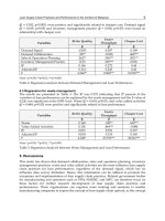
In Table 4.2, we present summary statistics related to profitability for US agribusinesses.
The operating benefit of a typical US agribusiness has been 9.4% on average during the 35
years period. This number is above the average WACC of a public US American firm.
Clarke and De Silva (2003) present a summary of several studies, where re, the cost of equity
has been between 5 and 6%. The cost of debt, rd, is lower than re by definition (i.e., residual
risk and tax shield in equation 4.5).

8
ROIC minus WACC is referred to as Economic Value Added (EVA) margin
9
Financial analysts that emphasize the use of cash flows (e.g., cash flow from operations or free cash
flow) over accounting profits (e.g., NOPAT) might be tempted to estimate a cash flow metric scaled by
IC. As cash flows already include changes in working capital and/or CAPEX, the metric estimated by
using cash flows should not be compared with WACC for decision making purposes.
Inventories, Financial Metrics, Profits, and Stock Returns in Supply Chain Management

255
Mean Median CV
IC 550.333 75.892 0.14
NOPAT 79.246 275.543 3.48

ROIC 9.4% 10.4% 1.11
Notes: Data base characteristics explained in notes Table 4.1. IC and NOPAT are expressed in million
USD as of 2004. NOPAT is estimated as in equation 4.3. EBIT is COMPUSTAT item 178. Details of IC
estimations are specified in the notes at the bottom of Table 4.1. CV stands for coefficient of variation.
Table 4.2. Summary statistics of selected items for the US food supply chain for the
1970/2004 period
Market Value of the Firm
The market value of the firm (FV) captures not only the fundamental or accounting
characteristics of the enterprise, but also investors ' expectations. This metric is defined as,

FV MCap D C
=
+−, (4.8)
where MCap, market capitalization, is defined as stock price times the number of shares
outstanding. While in IC (equation 4.1) equity is assessed at book value, in FV this value is
"updated" according to what investors believe the firm's equity is worth at market value.
10

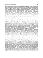
In Table 4.3 we present summary statistics of the book value of equity and its market value
for the US food sector.

Mean Median Std. Dev. CV
Book Value of Equity 309.304 46.809 1,052.086 3.40
Market Capitalization 1,127.496 62.329 6,082.294 5.39
Market Firm Value 1,368.525 99.374 6,582.137 4.81
P/BV 2.358 1.327 15.096 6.40
Note: Data base characteristics explained in notes Table 4.1. Values in million USD as of 2004, expect
P/BV, the stock price divided by the book value of shares. Market capitalization is stock price at the end
of calendar year, COMPUSTAT item 24 times number of common shares outstanding, COMPUSTAT
item 25. The book value of equity is COMPUSTAT item 60.

Table 4.3. Summary statistics of selected items for the US food supply chain for the
1970/2004 period
In the following section we investigate how inventories and other IC components affect the
market value of firms. To proxy the market value of equity we use stock returns or the
changes in stock prices. Annual stock returns are estimated by compounding monthly
returns obtained from the CRSP data base. Further, we compare IC components in t with
stock returns in t+1 to assess the reaction of investors to reported financial metrics.

10
Debt could also be considered at market value. But since debt securities are not as liquid as equities, it
is common to use the book value of debt. In addition, in equation 4.9 financial analysts make an
adjustment, especially for firms consolidating results from their subsidiaries. Thus, it is common to
multiply the multiple P/BV by Minority Interest (Equity, in the balance sheet).