Supply Chain Management Part 10 pptx

16
Towards Improving Supply Chain Coordination
through Business Process Reengineering
Marinko Maslaric
1
and Ales Groznik
2
1
University of Novi Sad, Faculty of Technical Sciences
2
University of Ljubljana, Faculty of Economics
1
Serbia
2
Slovenia
1. Introduction
Global marketplaces, higher levels of product variety, shorter product life cycles, and demand
for premium customer services are all things which cause pressure for one supply chain to be
more efficient, more time compressed and more cost effective. This has become even more
critical in recent years because the advancement in information technology has enabled
companies to improve their supply chain strategies and explore new models for management
of supply chain activity. Among others, important research area in the supply chain
management literature is the coordination of the supply chain. Actually, the understanding
and practicing of supply chain coordination has become an essential prerequisite for staying
competitive in the global race and for enhancing profitability. Hence, supply chain
management needs to be defined to explicitly recognise the strategic nature of coordination
and information sharing between trading partners and to explain the dual purpose of supply
chain management: to improve the performance of an individual organisation an to improve
the performance of the whole supply chain. In this context, we present the business process
reengineering as a tool for achievinging effective supply chain management, and illustrate
through a case study how business process modelling can help in achieving successful

improvements in sharing information and the coordination of supply chain processes.
It is well recognised that advances in information technologies have driven much change
through supply chain and logistics management services. Traditionally, the management of
information has been somewhat neglected. The method of information transferring carried out
by memebers of the supply chain has consisted of placing orders with the member directly
above them. This caused many problems in the supply chain including: excessive inventory
holding, longer lead times and reduced service levels in addition to increased demand
variability or the ‘Bullwhip Effect’. Thus, as supply chain management progresses, supply
chain managers are realising the need to utilise improved information sharing throughout the
supply chain in order to have coordinated supply chain and to remain competitive. However,
coordination is not just a mere information sharing. Information can be shared but there may
not be any alignment in terms of incentives, objectives and decisions (Lee et al., 1997b).
Coordination involves alignments of decisions, objectives and incentives and this can be done
only through new reengineered business process models, which need to follow the
information sharing. Appropriate business processes are a prerequisite for the strategic
Supply Chain Management

352
utilisation of information sharing, because the simple use of information technology
applications to improve information transfers between supply chain members is not in itself
enough to realise the benefits of information sharing. A mere increase in information transfers
does not mean that information distortions (Bullwhip Effect) will be avoided and the efficiency
of logistics processes will be improved. The business models of existing processes have to be
changed so as to facilitate the better use of the information transferred (Trkman et al., 2007). In
this chapter, by using business process modelling and simulation we show how achieving
only successful business process changes can contribute to the full utilisation of improved
information sharing, and so to the full coordination of the supply chain. In accordance with the
above, the main goals of this chapter are:
• To develop strategic connection between information sharing and supply chain
coordination through business process reengineering;

• To present how only full coordinated supply chains can increase supply chain
performances as costs and value of Bullwhip Effect;
• To promote value of Bullwhip Effect as a universal performance for supply chain
coordination;
• To connect existing theoretical studies with a real-life complex case study, in an attempt
to provide people in the working world with the expected performance improvements
discussed in this chapter.
In order to achieve these goals, this chapter analyse a two-level supply chain with a single
supplier who supplies products to a retailer who, in turn, faces demands from the end
customer. In addition, a discrete events simulation model of the presented supply chain has
been developed.
The organisation of the rest of this chapter is as follows: The next two sections briefly review
related literature about the key concepts of the chosen topic. Section 4 formulates the case
study and outlines business process models for the current and proposed state for the
company under consideration. Section 5 details a simulation study with experimentation
concerning information sharing, business process models and a type of inventory control,
while Section 6 discusses the results and concludes.
2. Supply chain coordination
2.1 Background
A supply chain is the set of business processes and resources that transforms a product from
raw materials into finished goods and delivers those goods into the hands of the customer.
Supply chain management has been defined as ‘the management of upstream and
downstream relationship with suppliers, distributors and customers to achieve greater
customer value-added at less total cost’ (Wilding, 2003). The objective of supply chain
management is to provide a high velocity flow of high quality, relevant information that
enables suppliers to provide for the uninterrupted and precisely timed flow of materials to
customers. Supply chain excellence requires standardised business processes supported by a
comprehensive data foundation, advanced information technology support and highly
capable personnel. It needs to ensure that all supply chain practitioners’ actions are directed
at extracting maximum value. According to (Simchi-Levi et al., 2003), supply chain

management represents the process of planning, implementing and controlling the efficient,
cost-effective flow and storage of raw materials, in-process inventory, finished goods, and
related information from the point of origin to the point of consumption for the purpose of
Towards Improving Supply Chain Coordination through Business Process Reengineering

353
meeting customers’ requirements. The concept of supply chain management has received
increasing attention from academicians, consultants and business managers alike (Tan et al.,
2002; Feldmann et al., 2003; Croom et al., 2000; Maslaric, 2008). Many organisations have
begun to recognise that supply chain management is the key to building sustainable
competitive edge for their products and/or services in an increasingly crowded marketplace
(Jones, 1998). However, effective supply chain management requires the execution of a
precise set of actions. Unfortunately, those actions are not always in the best interest of the
members in the supply chain, i.e. the supply chain members are primarily concerned with
optimising their own objectives, and that self serving focus often results in poor
performance. Hence, optimal performance and efficient supply chain management can be
achieved if the members of supply chain are coordinated such that each member’s objective
becomes aligned with the supply chain’s objective.
According to (Merriam-Webster, 2003), coordination is a process to bring into a common
action, movement or condition, or to act together in a smooth concerted way. Coordination
is studied in many fields: computer science, organisation theory, management science,
operations research, economics, linguistic, psychology, etc. In all of those fields,
‘coordination’ deal with similar problems and some of that knowledge might be utilised in
the research of supply chain coordination. Coordination issues in supply chain are
discussed in the literature in various ways including supply chain coordination (Lee et al.,
1997a), channel integration (Towill et al., 2002), strategic alliance and collaboration
(Bowersox, 1990; Kanter, 1994), information sharing and supply chain coordination (Lee et
al., 1997a; Lee et al., 1997b; Chen et al., 2000), collaborative planning, forecast and
replenishment (Holmstrom et al., 2002), and vendor-managed inventory (Waller et al., 1999).
In general, supply chain coordination can be accomplished through centralisation of

information and/or decision-making, information sharing and incentive alignments.
Various analyses on different coordination mechanisms have been carried out to develop
optimal solutions for coordinating supply chain system decisions and objectives. Most
literature addresses coordination problems in the following three situations (Sahin &
Robinson, 2002): (1) decentralised or centralised decision-making; (2) full, partial, or no
information sharing; (3) coordination or no coordination. For the purpose of the present
chapter, we will review situations belonging to the second category, information sharing.
2.2 Information sharing
Coordination between the different companies is vital for success of the global optimisation of
the supply chain, and it is only possible if supply chain partners share their information. In
traditional supply chains, members of the chain make their own decision based on their
demand forecast and their cost structure. So, many supply chain related problems such as
Bullwhip Effect can be attributed to a lack of information sharing among various members in
the supply chain. Sharing information has been recognised as an effective approach to
reducing demand distortion and improving supply chain performance (Lee et al., 1997a).
Accordingly, the primary benefit of sharing demand and inventory information is a reduction
in the Bullwhip Effect and, hence, a reduction in inventory holding and shortage costs within
supply chain. The value of information sharing within a supply chain has been extensively
analysed by researches. Various studies have used a simulation to evaluate the value of
information sharing in the supply chains (Towill et al., 1992; Bourland et al., 1996; Chen, 1998;
Gavirneni et al., 1999; Dejonckheere et al., 2004; Ferguson & Ketzenberg, 2006). Detailed
information about the amount and type of information sharing can be found in (Li et al., 2005).
Supply Chain Management

354
The existing literature has investigated the value of information sharing as a consequence of
implementing modern information technology. However, the formation of a business model
and utilisation of information is also crucial. Information should be readily available to all
companies in supply chains and the business processes should be structured so as to allow
the full use of this information (Trkman et al., 2007). One of the objectives of this chapter is

to offer insights into how the value of information sharing within a two-level supply chain is
affected when two different models of business process reengineering are applied.
Moreover, the literature shows that, although numerous studies have been carried out to
determine the value of information sharing, little has been published on real systems. The
results in this chapter have been obtained through a study of a real-life supply chain case
study using simulation.
2.3 Bullwhip effect
Behind the objectives regarded to developing strategic connection between information
sharing and supply chain coordination through business process reengineering and
connecting existing theoretical studies with a real-life case study, this chapter has two more
objectives. First, to examine the impact of information sharing with combinations of different
inventory control policies on Bullwhip Effect and inventory holding costs, and second, to
promote value of Bullwhip Effect as a common performance for supply chain coordination.
The Bullwhip Effect is a well-known phenomenon in supply chain management. In a single-
item two-echelon supply chain, it means that the variability of the orders received by the
manufacturer is greater than the demand variability observed by the retailer. This
phenomenon was first popularised by Jay Forrester (1958), who did not coin the term
bullwhip, but used industrial dynamic approaches to demonstrate the amplification in
demand variance. At that time, Forrester referred to this phenomenon as ‘Demand
Amplification’. Forrester’s work has inspired many researchers to quantify the Bullwhip
Effect, to identify possible causes and consequences, and to suggest various
countermeasures to tame or reduce the Bullwhip Effect (Boute & Lambrecht, 2007). One of
those researchers is Lee (Lee et al., 1997a; Lee et al., 1997b) who named this phenomenon as
‘Bullwhip Effect’ and who identified the main causes of the Bullwhip Effect and offered
solutions to manage it. They logically and mathematically proved that the key causes of the
Bullwhip Effect are: (1) demand forecasting updating; (2) order batching; (3) price
fluctuation; and (4) shortage gaming. According to this researcher, the key to managing the
Bullwhip Effect is to share information with the other members of the supply chain. In these
papers, they also highlighted the key techniques to manage the Bullwhip Effect.
A number of researchers designed games to illustrate the Bullwhip Effect. The most famous

game is the ‘Beer Distribution Game’. This game has a rich history: growing out of the
industrial dynamics work of Forrester and others at MIT, it is later on developed by Sterman
in 1989. The Beer Game is by far the most popular simulation and the most widely used
games in many business schools, supply chain electives and executive seminars. Simchi-Levi
et al., (1998) developed a computerized version of the Beer Game, and several versions of
the Beer Game are nowadays available, ranging from manual to computerized and even
web-based versions (Jacobs, 2000).
We can measure the Bullwhip Effect in different ways, but for the purpose of this research
we accepted the measures applied in (Fransoo & Wouters, 2000). We measure the Bullwhip
Effect as the quotient of the coefficient of variation of demand generated by one echelon(s)
and the coefficient of variation of demand received by this echelon:
Towards Improving Supply Chain Coordination through Business Process Reengineering

355

out
in
c
w
c
= (1)
where:

(
)
(
)
()
()
,

,
out
out
out
DttT
c
DttT
σ
μ
+
=
+
(2)
and:

()
(
)
()
()
,
,
in
in
in
DttT
c
DttT
σ
μ

+
=
+
(3)
D
out
(t,t+T) and D
in
(t,t+T) are the demands during time interval (t,t+T). For detailed
information about measurement issues, see (Fransoo & Wouters, 2000).
3. Business process reengineering
3.1 Background
The key to supply chain coordination is not ‘copy-pasting’ best practice, which assume
implementation of new information technology, from one company to another. Given the
unique context in which each supply chain operates, the key to full coordination lies in the
application of a context specific solution which is mostly regarded to business processes of
the company.
The business process is a set of related activities which make some value by transforming
some inputs into valuable outputs. In reengineering theories, organisational structures are
redesign by focusing on business processes and their outcome. Business process reengineering
may be seen as an initiative of the 1990s, which was of interest to many companies. The initial
drive for reengineering came from the desire to maximize the benefits of the introduction of
information technology and its potential for creating improved cross-functional integration in
companies (Davenport & Short, 1990). Business redesign was also identified as an opportunity
for better IT integration both within a company and across collaborating business units in a
study in the late 1980s conducted at MIT. The initiative was rapidly adopted and extended by
a number of consultancy companies and ‘gurus’ (Hammer, 1990). In business process
reengineering, a business process is seen as a horizontal flow of activities while most
organisations are formed into vertical functional groupings sometimes referred to in the
literature as ‘functional silos’. Business process reengineering by definition radically departs

from other popular business practices like total quality management, lean production,
downsizing, or continuous improvement. Business process reengineering is based on efficient
use of information technology, hence companies need to invest large amount of money the
achieve information technology enabled supply chain. Implemenation of new information
technology is necessary, but no means sufficient condition for enable efficient and cheap
information transfers. Business process reengineering is concerned with fundamentally
rethinking and redesigning business processes to obtain dramatic and sustaining
improvements in quality, costs, services, lead times, outcomes, flexibility and innovation. In
support of this, technological change through the implementation of simulation modelling is
being used to improve the efficiency and consequently is playing a major role in business
process reengineering (Cheung & Bal, 1998).
Supply Chain Management

356
3.2 Business process modelling
A business process model is an abstraction of business that shows how business
components are related to each other and how they operate. Its ultimate purpose is to
provide a clear picture of the enterprise’s current state and to determine its vision for the
future. Modelling a complex business requires the application of multiple views. Each view
is a simplified description (an abstraction) of a business from a particular perspective or
vantage point, covering particular concerns and omitting entities not relevant to this
perspective. To describe a specific business view process mapping is used. It consists of
tools that enable us to document, analyse, improve, streamline, and redesign the way the
company performs its work. Process mapping provides a critical assessment of what really
happens inside a given company. The usual goal is to define two process state: AS-IS and
TO-BE. The AS-IS state defines how a company’s work is currently being performed. The
TO-BE state defines the optimal performance level of ‘AS-IS’. In other words, to streamline
the existing process and remove all rework, delay, bottlenecks and assignable causes of
variation, there is a need to achieve the TO-BE state. Business process modelling and the
evaluation of different alternative scenarios (TO-BE models) for improvement by simulation

are usually the driving factors of the business renovation process (Bosilj-Vuksic et al., 2002).
In the next section a detailed case study is presented.
4. A case experience of business process reengineering
The case study is a Serbian oil downstream company. Its sales and distribution cover the full
range of petroleum products for the domestic market: petrol stations, retail and industries.
The enterprise supply chain comprises fuel depot-terminal (or distribution centre), petrol
stations and final customers. The products are distributed using tank tracks. The majority of
deliveries is accomplished with own trucks, and a small percentage of these trucks is hired.
The region for distribution is northern Serbia. It is covered by two distribution centres and
many petrol stations at different locations. In line with the aim of the chapter only a
fragment, namely the procurement process, will be shown in the next section. Presented
model was already used in (Groznik & Maslaric, 2010), and a broader description of the case
study can be found in (Maslaric, 2008).
From the supply chain point of view, the oil industry is a specific business, and for many
reason it is still generally based on the traditional model. The product is manufactured,
marketed, sold and distributed to customers. In other industries, advanced supply chain
operation is becoming increasingly driven by demand-pull requirements from the customer.
There is a strong vertically integrated nature of oil companies and that may be a potential
advantage. In other industries, much attention is focused on value chain integration across
multiple manufacturers, suppliers and customers. In the oil industry, more links in the chain
are ‘in house’, suggesting simpler integration. In practice, there is still a long way to go to
achieve full integration in the oil supply chain.
4.1 AS-IS model development
The next section covers the modelling of the existing situation (AS-IS) in the procurement
process of the observed downstream supply chain case study. The objective was to map out
in a structured way the distribution processes of the oil company. The modelling tools used
in this case study come from the Igrafx Process. These modelling tools were applied in order
to identify the sequence of distribution activities, as well as the decisions to be taken in
Towards Improving Supply Chain Coordination through Business Process Reengineering

357
various steps of the distribution process. The AS-IS model was initially designed so that the
personnel involved in the distribution processes could review them, and after that the final
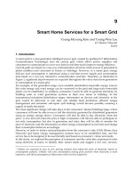
model shown in Figure 1 was developed.


Fig. 1. AS-IS model of the process
Supply Chain Management

358
The core objective of supply chains is to deliver the right product at the right time, at the
right price and safely. In a highly competitive market, each aims to carry this out more
effectively, more efficiently and more profitably than the competitors. Because both the
prices and quality of petrol in Europe are regulated, the main quality indicator in oil supply
chains is the number of stock-outs. The main cost drivers are therefore: number of stock-
outs, stock level at the petrol station and process execution costs. Lead time is defined as the
time between the start (measurement of the stock level) and the end (either the arrival at a
petrol station or the decision not to place an order) of the process (Trkman et al., 2007).
The main problems identified when analysing the AS-IS model relate to the company’s
performance according to local optimisation instead of global optimisation. The silo mentality
is identified as a prime constraint in the observed case study. Other problems are in inefficient
and costly information transfer mainly due to the application of poor information technology.
There is no optimisation of the performance of the supply chain as a whole. Purchasing,
transport and shipping are all run by people managing local, individual operations. They have
targets, incentives and local operational pressures. Everything was being done at the level of
the functional silo despite the definition that local optimisation leads to global deterioration.
The full list of problems identified on tactical and strategic levels are identical to those in
(Trkman et al., 2007), so for greater detail see that paper. Based on the mentioned problems,
some improvements are proposed. The main changes lie in improved integration of whole
parts of the supply chain and centralised distribution process management.

4.2 TO-BE models development
The emphasis in business process reengineering is put on changing how information
transfers are achieved. A necessary, but no means sufficient condition for this is to
implement new information technologies which enable efficient and cheap information
transfers. Hence, information technology support is not enough as deep structural and
organisational changes are needed to fully realise the potential benefits of applying new
information technology. In this case study we develop two different propositions for
business process reengineering (two TO-BE models) to show how implementation of new
information technology without business process renovation and the related organisational
changes does not mean the full optimisation of supply chain performance.
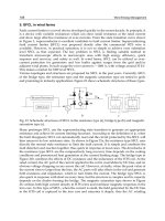
The first renewed business model (TO-BE 1) is shown in Figure 2 and represents the case of
implementing information technology without structural changes to business processes. In the
TO-BE 2 model, there is no integrated and coordinated activity through the supply chain.
Inventory management at the petrol stations and distribution centre is still not coordinated.
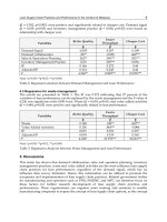
The TO-BE 2 model assumes that the processes in the whole downstream oil supply chain
are full integrated and the distribution centre takes responsibility for the whole procurement
process. The TO-BE 2 business model is shown in Figure 3. The main idea is that a new
organisational unit within the distribution centre takes on a strategic role in coordinating
inventory management and in providing a sufficient inventory level at the petrol stations
and distribution centre to fulfil the demand of the end customer. It takes all the important
decisions regarding orders in order to realise this goal. Other changes proposed in the TO-
BE 2 model are the automatic measurement of petrol levels at petrol stations and the
automatic transfer of such data to the central unit responsible for petrol replenishment; the
predicting of future demand by using progressive tools; and using operations research
methods to optimise the transportation paths and times. The role of information technology
in all of these suggestions is crucial.
Towards Improving Supply Chain Coordination through Business Process Reengineering

359

Fig. 2. TO-BE 1 model of the process
4.3 Measuring the effect of reengineering
The effect of the changes can be estimated through simulations. Because our study has two
kinds of objective, we have two kind of simulations. In our first example we simulated
business processes to investigate the impact of business process reengineering on the
information sharing value, measured by lead times and transactional costs. The second
simulation, which partly uses the results of the first simulation, represents an object-
oriented simulation which helps define the impact of information sharing and appropriate
inventory control on the Bullwhip Effect and inventory holding costs in the oil downstream
supply chain under consideration. Both simulations are especially important as they enable
us to estimate the consequence of possible experiments.
In the first simulation we estimated changes in process execution costs and lead times. First
a three-month simulation of the AS-IS and of both the TO-BE models was run. In the AS-IS
model a new transaction is generated daily (the level of petrol is checked once a day), and in
the TO-BE it is generated on an hourly basis (the level of stock is checked automatically
every hour). The convincing results are summarised in Table 1. The label ‘Yes’ refers to

Supply Chain Management

360

Fig. 3. TO-BE 2 model of the process
those transactions that lead to the order and delivery of petrol, while the label ‘No’ means a
transaction where an order was not made since the petrol level was sufficient. The average
process costs are reduced by almost 50%, while the average lead time is cut by 62% in the
case of the TO-BE 2 business model. From this it is clear that this renovation project is
justifialbe from the cost and time perspectives. The results in Table 1 show that a full
improvement in supply chain performances is only possible in the case of implementing
both new information technology which enables efficient information sharing, and the
redesign of business processes. The mere implementing of information technologies without

structural and organisational changes in business processes would not contribute to
realising the full benefit.

Transaction No. Av. lead-time
(hrs)
Av. work
(hrs)
Av. wait
(hrs)
Average
costs (€)
Yes (AS-IS) 46 33.60 11.67 21.93 60.10
No (AS-IS) 17 8.43 2.40 6.03 8.47
Yes (TO-BE 1) 46 27.12 10.26 16.86 56.74
No (TO-BE 1) 1489 0.00 0.00 0.00 0.00
Yes (TO-BE 2) 46 12.85 4.88 7.98 32.54
No (TO-BE 2) 1489 0.00 0.00 0.00 0.00
Table 1. Comparasion of simulation results for the AS-IS and TO-BE models
Towards Improving Supply Chain Coordination through Business Process Reengineering

361
The results of the previous simulation (lead time) were used as an input for the next
simulation so as to help us find the impact of information sharing on the Bullwhip Effect
and inventory holding costs in the observed supply chain.
5. Inventory control simulation
In this section we employed an object-oriented simulation to quantify the benefit of
information sharing in the case study. The system in our case study is a discrete one since
supply chain activities, such as order fulfilment, inventory replenishment and product
delivery, are triggered by customers’ orders. These activities can therefore be viewed as
discrete events. A three-month simulation of the level of stock at a petrol station that is open

24 hours per day was run.
In order to provide results for the observed supply chain performance, the following
parameters are set:
•
Demand pattern: Historical demand from the end customer to petrol stations and from
petrol stations to distribution centres was studied. From this historical demand, a
probability distribution was created.
•
Forecasting models: The exponential smoothing method was used to forecast future
demand.
•
Information sharing: Two different types of information sharing were considered: (1) No
IS-no information sharing (AS-IS model); and (2) IS-full information sharing (TO-BE
models).
•
Lead time: Lead time from the previous simulation business process was used.
•
Inventory control: Three types of inventory replenishment policy were used: (1) No
inventory policy based on logistical principles. There was a current state in the viewed
supply chain (AS-IS model); (2) The petrol station and distribution centre implement
the (s, S) inventory policy according to demand information from the end customer, but
the distribution centre was not responsible for the petrol station’s replenishment policy
– no VMI policy (TO-BE 1 model); and (3) VMI – full information sharing is adopted
and the distribution centre is in charge of the inventory control of the petrol station. The
one central unit for inventory control determines the time for replenishment as well as
the quantities of replenishment (TO-BE 2 model).
•
Inventory cost: This is the cost of holding stocks for one period.
•
Bullwhip Effect: The value of the Bullwhip Effect is measured from equations (1), (2) and

(3).
When we talk about inventory control, regular inventories with additional safety stock are
considered. These are the inventories necessary to meet the average demand during the time
between successive replenishment and safety stock inventories are created as a hedge
against the variability in demand for the inventory and in replenishment lead time. The
graphical representation of the above mentioned inventory control method is depicted in
Figure 4 (Groznik & Maslaric, 2009; Petuhova & Merkuryev, 2006).
The inventory level to which inventory is allowed to drop before a replacement order is
placed (reorder point level) is found by a formula:

()* ()* *sEX LTSTDX LTz=+ (4)
Supply Chain Management

362

Fig. 4. Inventory control method

where:
LT – lead time between replenishment;
() ()STD X D X= - standard deviation of the mean demand;
z – the safety stock factor, based on a defined in-stock probability during the lead time.
The total requirements for the stock amount or order level S is calculated as a sum of the
reorder point level and a demand during the lead time quantity:
S = s + E(X)*LT (5)
The order quantity Q
i
is demanded when the on-hand inventory drops below the reorder
point and is equal to the sum of the demand quantities between the order placements:
Q
i

= X
1
+ X
i
+ +X
v
(6)
Where v is random variable, and represents a number of periods when an order is placed.
While the demand X is uncertain and implementing such a type of inventory control
method, placed order quantity Q is expected to be a random variable that depends on the
demand quantities.
To investigate the effect of information sharing upon supply chain performance (Bullwhip
Effect and inventory costs), three scenarios are designed with respect to the above
parameters:
•
Scenario 1: No IS, no defined inventory control, (AS-IS model);
•
Scenario 2: IS, no VMI, (TO-BE 1) model; and
•
Scenario 3: IS, VMI, (TO-BE 2) model.
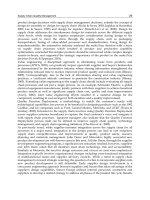
The simulation was run using GoldSim Pro 9.0. The performance measures derived from the
simulation results are summarised in Figure 5 and Figure 6. The results from Figure 5 show
Towards Improving Supply Chain Coordination through Business Process Reengineering

363
that the value of the Bullwhip Effect is smallest for Scenario 3, which assumed full
information sharing with appropriate structural changes of business processes, and full
coordination in inventory control across the supply chain. These results also show that fully
utilising the benefit of implementing information technology and inventory management
based on logistical principles can decrease the value of Bullwhip Effect by 28% in the

observed case study.


100
75
72
0
20
40
60
80
100
(%)
Scenario 1 Scenario 2 Scenario 3


Fig. 5. Bullwhip effect value comparasion of three scenarios
In Figure 6 a comparison of inventory costs with regard to the scenarios is shown. The
minimum inventory holding costs are seen in Scenario 3, like in the first case. The result
from Figure 5 show that benefits from the application of new information technology,
business process reengineering and coordinated inventory policy, expressed by decreasing
inventory holding costs, could be 20%.


100
92
79,8
0
20
40

60
80
100
(%)
Scenario 1 Scenario 2 Scenario 3


Fig. 6. Inventory costs comparasion of three scenarios
Supply Chain Management

364
6. Conclusion
Supply chain management has become a powerful tool for facing up to the challenge of
global business competition because supply chain management can significantly improve
supply chain performance. This chapter explores how achieving only successful business
process changes can contribute to the full utilisation of improved sharing, and so to the full
coordination of the supply chain. The conclusions of the simulation experiments are:
information sharing can enhance the performance of the supply chain. In addition, business
process reengineering and coordination are also important mechanisms in the supply chain
to improve performance. Coordination can reduce the influence of the Bullwhip Effect and
improve cost efficiency. In the previous literature there were not many connections between
theoretical studies and a real-life complex case study. This chapter is hence one of the few
attempts in this direction. This research represents a part of the project financed by the
Ministry of Serbia.
7. References
Bosilj-Vuksic, V.; Indihar-Stemberger, M.; Jaklic, J. & Kovacic, A. (2002). Assessment of E-
Business Transformation using Simulation Modelling. Simulation, Vol. 78, No. 12,
pp. 731-744, ISSN: 0037-5497
Bourland, K.; Powell, S. & Pyke, D. (1996). Exploring Timely Demand Information to Reduce
Inventories. European Journal of Operational Research, Vol. 44, No. 2, pp. 239-253,

ISSN: 0377-2217
Boute, R.N. & Lambrecht, M.R. (2007). Exploring the Bullwhip Effect by Means of
Spreadsheet Simulation. Vlerick Leuven Gent Working Paper Series, Vol. 4, pp. 1-33,
Vlerick Leuven Gent Management School, Leuven
Bowersox, D.J. (1990). The Strategic Benefits of Logistics Alliances. Harvard Business Review,
Vol. 68, No. 4, pp. 36-45, ISSN: 0017-8012
Chen, F. (1998). Echelon Reorder Point, Installation Reorder Points, and the Value of
Centralized Demand Information. Management Science, Vol. 44, No. 12, pp. 221-234,
ISSN: 0025-1909
Chen, F.; Drezner, Z.; Ryan, J.K. & Simchi-Levi, D. (2000). Quantifying the Bullwhip Effect in
a Simple Supply Chain: the Impact of Forecasting, Lead Times, and Information.
Management Science, Vol. 46, No. 3, pp. 436-443, ISSN: 0025-1909
Cheung, Y. & Bal, J. (1998). Process Analysis Techniques and Tools for Business
Improvement. Business Process Management Journal, Vol. 4, No. 4, pp. 274-290, ISSN:
1463-7154
Croom, S.; Romano, P. & Giannakis, M. (2000). Supply Chain Management: An Analytical
Framework for Critical Literature Review. European Journal of Purchasing and Supply
Management, Vol. 6, No. 1, pp. 67-83, ISSN: 0969-7012
Davenport, T.H. & Short, J. (1990). The New Industrial Engineering: Information
Technology and Business Process Redesign. Sloan Management Review, Vol. 34, No.
4, pp. 11-27, ISSN: 0019-848X
Dejonckheere, J.; Disney, S.M.; Lambrecht, M.R. & Towill, D.R. (2004). The Impact of
Information Enrichment on the Bullwhip Effect in Supply Chains: a Control
Theoretic Approach. European Journal of Operational Research, Vol. 153, No. 3, pp.
727-750, ISSN: 0377-2217
Towards Improving Supply Chain Coordination through Business Process Reengineering

365
Feldman, M. & Miler, S. (2003). An Incentive Scheme for True Information Providing in
Supply Chains. Omega, Vol. 31, No. 2, pp. 63-73, ISSN: 0305-0483

Ferguson, M. & Ketzenberg, M.E. (2006). Information Sharing to Improve Retail Product
Freshness of Perishables. Production and Operations Management, Vol. 15, No. 1, pp.
57-73, ISSN: 1937-5956
Fransoo, J.C. & Wouters, M.J.F. (2000). Measuring the Bullwhip Effect in the Supply Chain.
Supply Chain Management: An International Journal, Vol. 5, No. 2, pp. 78-89, ISSN:
1359-8546
Gavirneni, S.; Kapuscinski, R. & Tayur, S. (1999). Value of Information in Capacitated
Supply Chains. Management Science, Vol. 45, No. 1, pp. 16-24, ISSN: 0025-1909
Groznik, A. & Maslaric, M. (2009). Investigating the Impact of Information Sharing in a
Two-Level Supply Chain Using Business Process Modelling and Simulation: A
Case Study, Proceedings of 23
rd
European Conference on Modelling and Simulation, pp.
39-45, ISBN: 0-9553018-8-2, Madrid, June 2009, European Council for Modelling
and Simulation, Madrid
Groznik, A. & Maslaric, M. (2010). Achieving Competitive Supply Chain Through Business
Process Re-engineering: A Case from Developing Country. African Journal of
Business Management, Vol. 4, No. 2, pp. 140-148, ISSN: 1990-3839
Hammer, M. (1990). Reengineering Work: Don’t automate obliterate. Harvard Business
Review, Vol. 64, No. 4, pp. 104-112, ISSN: 0017-8012
Holmstrom, J.; Hameri, A.P.; Nielsen, N.H.; Pankakoshi, J. & Slotte, J. (1997). Examples of
Production Dynamics Control for Cost Efficiency. International Journal of Production
Economics, Vol. 48, No. 2, pp. 109-119, ISSN: 0925-5273
Jacobs, F.R. (2000). Playing the Beer Distribution Game over the Internet. Production and
Operations Management, Vol. 9. No. 1, pp. 31-39, ISSN: 1937-5956
Jones, C. (1998). Moving Beyond ERP: Making the Missing Link. Logistics Focus, Vol. 6, No.
7, pp. 187-192, ISSN: 1350-6293
Kanter, R.M. (1994). Collaborative Advantage: the Art of Alliances, Harvard Business Review,
Vol. 72, No. 4, pp. 96-112, ISSN: 0017-8012
Lee, H.L.; Padmanabhan, P. & Whang, S. (1997a). The Bullwhip Effect in Supply Chain.

Sloan Management Review, Vol. 38, No. 3, pp. 93-102, ISSN: 0019-848X
Lee, H.L.; Padmanabhan, P. & Whang, S. (1997b). Information Distortion in a Supply Chain:
the Bullwhip Effect. Management Science, Vol. 43, No. 4, pp. 546-558, ISSN: 0025-
1909
Li, J.; Sikora, R.; Shaw, M.J. & Tan, G.W. (2005). A Strategic Analysis of Inter-organizational
Information Sharing. Decision Support Systems, Vol. 42, pp. 251-266, ISSN: 0167-9236
Maslaric, M. (2008). An Approach to Investigating the Impact of Information Charasteristic
on Logistic Processes Planning and Coordination in Supply Chains. Master Thesis.
University of Novi Sad, Serbia
Merriam-Webster. (2003). Merriam-Webster Collegiate Dictionary, 11
th
ed., Merriam-
Webster
Petuhova, J. & Merkuryev, Y. (2006). Combining Analytical and Simulation Approaches to
Quantification of the Bullwhip Effect. International Journal of Simulation, Vol. 8, No.
1, pp. 16-24, ISSN: 1473-8031
Supply Chain Management

366
Sahin, F. & Robinson, E.P. (2002). Flow Coordination and Information Sharing in Supply
Chains: Review, Implications, and Directions for Future Research. Decision Science,
Vol. 33, No. 4, pp. 505-536, ISSN: 0011-7315
Simchi-Levi, D.; Kaminsky, P. & Simchi-Levi, E. (1998). Designing and Managing the Supply
Chain. Irwin/McGraw-Hill Professional. ISBN: 0-07-284553-8, New York, USA
Simchi-Levi, D.; Kaminsky, P. & Simchi-Levi, E. (2003). Managing the Supply Chain: The
Definitive Guide for the Business Professional. McGraw-Hill Professional. ISBN: 0-07-
141031-7, New York, USA
Tan, K.C.; Lyman, S.B. & Wisner, J.D. (2002). Supply Chain Management: a Strategic
Perspective. International Journal of Operations and Production Management, Vol. 22,
No. 6, pp. 614-631, ISSN: 0144-3577

Towill, D.R.; Naim, N.M. & Wikner, J. (1992). Industrial Dynamics Simulation Models in the
Design of Supply Chains. International Journal of Physical Distribution and Logistics
Management, Vol. 22. No. 5, pp. 3-13, ISSN: 0960-0035
Towill, D.R.; Childerhouse, P. & Disney, S.M. (2002). Integrating the Automotive Supply
Chain: Where are We Now? International Journal of Physical Distribution & Logistics
Management, Vol. 32, No. 2, pp. 79-95, ISSN: 0960-0035
Trkman, P.; Stemberger, M.I.; Jaklic, J. & Groznik, A. (2007). Process Approach to Supply
Chain Integration. Supply Chain Management: An International Journal, Vol. 12, No. 2,
pp. 116-128, ISSN: 1359-8546
Waller, M.; Johnson, M.E. & Davis, T. (1999). Vendor-Managed Inventory in the Retail
Supply Chain. Journal of Business Logistics, Vol. 20, No. 1, pp. 183-204, ISSN: 0735-
3766
Wilding, R. (2003). The 3Ts of Highly Effective Supply Chains. Supply Chain Practice, Vol. 5,
No. 3, pp. 30-39, ISSN: 1466-0091
17
Integrated Revenue Sharing Contracts to
Coordinate a Multi-Period
Three-Echelon Supply Chain
Mei-Shiang Chang
Department of Civil Engineering, Chung Yuan Christian University
Taiwan
1. Introduction

A supply chain can be defined as a network of facilities and distribution options that
performs the functions of procurement of materials, transformation of these materials into
intermediate and finished products, and the distribution of these finished products to
customers. Different entities in a supply chain operate subject to different sets of constraints
and objectives under different industrial environments. Each member of a decentralized
supply chain has its own decision rights to optimize its costs or benefits. Recently, the topic
of decentralized supply chain modelling and analysis has been of great interest. Most of the

studies on decentralized supply chain modelling have focused on designing a mechanism to
fully integrate these individualistic decisions in order to ensure that the decision outcome of
an individual member of the supply chain is in accordance with the decision outcome of the
entire supply chain (Cachon & Lariviere, 2001; Moinzadeh and Bassok, 1998; Tsay et al., 1999).
Perfect coordination mechanisms allow the decentralized supply chain to perform as well as
a centralized one, in which all decisions are made by a single entity to maximize supply-
chain-wide profits. Several types of contractual agreements which may determine incentive
mechanisms to integrate a decentralized supply chain, inclunding profit sharing (Atkinson,
1979; Jeuland and Shugan, 1983), consignment (Kandel, 1996), buy-backs (Pasternack, 1985;
Emmons & Gilbert, 1987), quantity-flexibility (Tsay & Lovejoy, 1999), revenue sharing
(Giannoccaro & Pontrandolfo, 2004; Cachon & Lariviere, 2005; Chang & Hsueh, 2006, 2007),
revenue allocation rules (Shah et al., 2001), and quantity discounts (Dolan, 1987), etc.
One of these contractual agreements, revenue sharing is a mechanism that is gaining
popularity in practice and in research. Shah et al. (2001) have adopted Nash’s game theory
to formulate a model which explores a fair revenue allocation mechanism among the
members of a multi-tier supply chain. The model provides a compromise solution of
maximized revenue for each individual member of the supply chain under the inventory
and production constraints. Giannoccaro & Pontrandolfo (2004) have extended the revenue
sharing contract of two-tier to a three-tier supply chain model. Cachon & Lariviere (2005)
have presented the revenue sharing contract concept and discussed its influence on supply
chain performances. The revenue sharing contract can be described by two parameters,
retail price and retailers’ revenue retention ratio. Chang & Hsueh (2006, 2007) extended
Giannoccaro & Pontrandolfo (2004) to explore a three-tier supply chain integration problem
Supply Chain Management

368
with the time-varying multi-period demand and the constant price elasticity demand
function. Multiple objective programming techniques are applied to determine the revenue
sharing contract parameters, the purchasing price and revenue sharing ratios among the
members of the supply chain. In order to heighten the incentive cooperation, equilibrium

behaviors for decentralized supply chains are included and regarded as compromise
benchmarks for supply chain integration.
The remainder of this chapter is organized as follows. In Section 2, two multi-period three-
tier supply chain network models are presented. A equilibrium model of decentralized
supply chain network is introduced first. Herein the optimality conditions of the various
decision-makers are derived and formulated as a finite-dimensional variational inequality
model. A multi-objectives programming model to determine the revenue sharing constract
parameters is given next. In Section 3, a well-known solution algorithm, diagonalization
method, is presented to solve the variation inequility model of supply chain
networkequilibrium. In Section 4, a supply chain network example is provided for the
demonstration. Conclusions are given in the end.
2. Model formulation
The supply chain network is composed of m manufacturers, n distributors, and o retailers.
The other assumptions about the members of the supply chain network are summarized as
follows:
1. To accommodate changes in demand, the product inventory within this supply chain
network is stored at the manufacturers’ warehouses so that the manufacturers will have
sufficient inventory or production capacity to satisfy the distributors’ demand in the
current time period.
2. The total costs of the manufacturers have to bear are production cost, inventory cost and
transportation cost. The distributors are only responsible for the product handling and
purchasing costs. The retailers are directly associated with the market demand and
responsible for transportation costs and purchasing cost. All the cost functions for the
manufacturers, distributors, and retailers are continuous, convex, and nonlinear functions.
3. The demand function is a known function which can describe the relationship between
the market demand and market price.
2.1 Notations
()
k
dt:

The product demand of retailer k at time period t
()
i
f
e :
The production cost of manufacturer i at time period e
()
i
fe
:
The average production cost of manufacturer i at time period e
()
i
ht:
The inventory cost of manufacturer i at time period t
()
i
ht: The average inventory cost of manufacturer i at time period t
()
i
It:
The inventory level of manufacturer i at time period t
()
j
Lt:
The product quantity of distributor j at time period t
()
j
mt:
The product handling cost of distributor j at time period t

()
j
mt: The average product handling cost of distributor j at time period t
Integrated Revenue Sharing Contracts to Coordinate a Multi-Period Three-Echelon Supply Chain

369
()
i
qe:
The production quantity of manufacturer i at time period e
()
ij
q
t :
The product quantity delivered from manufacturer i to distributor j at time period
t
()
ijt
q
e :
The product quantity produced by manufacturer i at time period e and delivered
to distributor j at time period t
()
jk
q
t :
The product quantity delivered from distributor j to retailer k at time period t
()
ij
st

:
The transportation cost from manufacturer i to distributor j at time period t
()
ij
st
:
The average transportation cost from manufacturer i to distributor j at time period
t
()
jk
st:
The transportation cost from distributor j to retailer k at time period t
()
jk
st: The average transportation cost from distributor j to retailer k at time period t
i
j
T :
The leading time between manufacturer i and distributor j
j
k
T :
The leading time between distributor j and retailer k
,,
i
j
k
zzz
:
The profit for manufacturers, distributors, and retailers

***
,,
i
j
k
zzz:
The maximum profit for manufacturers, distributors, and retailers
,,
EEE
i
j
k
zzz:
The equilibrium profit for manufacturers, distributors, and retailers
3
k
φ
: The ratio of the retail revenues retained by retailer k
2
j
k
φ
:
The ratio of the wholesale revenue retained by distributor j, which is resulted
from the transaction between distributor j and retailer k
1
()
ij
t
ρ

:
The selling price of manufacturer i to distributor j at time period t
2
()
j
t
ρ
:
The selling price of distributor j at time period t
3
()
k
t
ρ
:
The selling price of retailer k at time period t
2.2 Market equilibrium model
Chang & Hsueh (2006) first focus on decision behaviours of manufacturers and then turn to
decision behaviours of distributors and retailers, subsequently. A complete equilibrium
model is finally constructed.
2.2.1 The manufacturers’ optimality conditions
Each manufacturer’s behaviour of seeking profit maximization can be expressed as follows.

1
ij
max () () () () ()
iijiiij
jt e t jt
tq t f e h t s t
πρ

=−−−
∑
∑∑∑
(1)
subject to
() ()
i ijt
jt
q
e
q
ee
=
∀
∑
(2)

,
() ()
i ijt
je t
It
q
et
<
=
∀
∑
(3)
Supply Chain Management

370

ij
ij
(-T)
-T
() () ,
ij ij t
et
qt q e jt
≤
=
∀
∑
(4)
( ) 0 , ,
ijt
q
e
j
te≥∀ (5)

1
( ) 0 ,
ij
t
j
t
ρ

≥∀ (6)
Eq. (1) designates that the profit of a manufacturer is the difference in total revenues and
total costs. Eq. (2) defines that the entire volume of production of manufacturer i at time
period e is equal to the sum of the quantities shipped from this manufacturer to all
distributors after time period e. Eq. (3) defines that the entire volume of inventory at time
period t is equal to the sum of the quantities produced by the manufacturer i before time
period t. Eq. (4) defines that the volume of transaction between manufacturer i and
distributor j at time period t is equal to the sum of the product quantity produced by
manufacturer i for distributor j before time period
i
j
tT
−
. Note that the production cost
()
i
fe
depends upon the entire volume of production at time period e. The inventory cost
()
i
ht depends upon the entire volume of inventory at time period t. The shared transaction
cost depends upon the volume of transaction at time period t. Eqs. (5) and (6) are
nonnegative constraints.
The manufacturers compete in a noncooperative fashion following Nash (1950, 1951). Each
manufacturer will determine this optimal production quantity, inventory quantity,
distribution quantity at each time period. The optimality conditions for all manufacturers
simultaneously expressed as Eq. (7).

1* *
*

*
*
***
1* *
( ) , if ( ) 0
()
()
()
, , ,
() () ()
( ) , if ( ) 0
ij ijt
ij
i
i
ijt ijt ijt
ij ijt
tqe
st
fe
ht
i
j
te
qe qe qe
tqe
ρ
ρ
⎧
=>

∂
∂
∂
⎪
++ ∀
⎨
∂∂∂
≥=
⎪
⎩
(7)
2.2.2 The distributors’ optimality conditions
Herein, each distributor’s behavior of seeking profit maximization can be expressed as
follows.

21
jij
max () () ( ) ( ) ()
jjk ijijijj
tk it t
tqt tTqtT mt
πρ ρ
=−−−−
∑
∑∑ ∑
(8)
subject to

() ( )
jijij

i
Lt
q
tT t
=
−∀
∑
(9)

( ) ( )
ij ij jk
ik
q
tT
q
tt
−
=∀
∑
∑
(10)
( ) 0 ,
ij
q
tit≥∀ (11)
() 0 ,
jk
q
tkt≥∀ (12)
Integrated Revenue Sharing Contracts to Coordinate a Multi-Period Three-Echelon Supply Chain

371

2
() 0
j
tt
ρ
≥∀ (13)
Eq. (8) designates that the profit of a distributor is the difference in total revenues and total
costs. Eq. (9) defines that the entire product quantity of distributor j at period t is equal to
the sum of purchase quantity from all manufacturers at the corresponding time period t-
i
j
T .
The handling cost
(
)
j
mt
depends upon the entire product quantity at period t. Eq. (10)
ensures that the received total product quantity of the distributor j from all manufacturers
departing at time period t-
i
j
T must be greater than or equal to the product quantity of the
distributor j which can be distributed to all retailers at time period t. Eqs. (11) ~ (13) are
nonnegative constraints.
Congenially, the distributors compete in a noncooperative manner, too. At each time
period, each distributor will determine the optimal order quantity with each manufacturer

as well as distribution quantity for each retailer. The optimality conditions for all
distributors satisfy Eqs. (14)~(16).

**
*
1*
*
**
( ) , if ( ) 0
()
( ) , ,
()
( ) , if ( ) 0
jijij
j
ij ij
ij ij
jijij
tqtT
mt
tT i
j
t
qtT
tqtT
γ
ρ
γ
⎧
=−>

∂
⎪
−+ ∀
⎨
−
≥−=
⎪
⎩
(14)

2* *
*
2* *
( ) , if ( ) 0
() , ,
( ) , if ( ) 0
jjk
j
jjk
tqt
t
j
kt
tqt
ρ
γ
ρ
⎧
=>
⎪

∀
⎨
≥=
⎪
⎩
(15)
() 0 ,
j
t
j
t
γ
≥∀ (16)
Note that ( )
j
t
γ
is the Lagrange multiplier associated with constraint (10) for distributor j at
time period t.
2.2.3 The retailers’ optimality conditions
On the analogy of the well-known spatial price equilibrium conditions, the equilibrium
conditions for each retailer at each time period can be stated as follows:

3* *
**
3* *
( ) , if ( ) 0
()() ,,
( ) , if ( ) 0
kjk

jjkjk
kjk
tqt
tT st
j
kt
tqt
ρ
ρ
ρ
⎧
=>
⎪
−+ ∀
⎨
≥=
⎪
⎩
(17)

*3*
*
*3*
( ) , if ( ) 0
() ,
( ) , if ( ) 0
jk jk k
j
k
jk jk k

j
qtT t
dt kt
qtT t
ρ
ρ
⎧
=− >
⎪
⎪
∀
⎨
≤− =
⎪
⎪
⎩
∑
∑
(18)
Eq. (17) ensures that the product will be distributed to the retailer k from distributor j at time
period t, if the price charged by the distributor j for the product at time period
j
k
tT−
plus
the transportation cost faced by retailer k at time period t doesn’t exceed the price that
consumers of retailer k are willing to pay for the product at time period t. Eq. (18) states that
the total product quantity distributed to the retailer k from all distributors at time period
Supply Chain Management

372
t
j
k
T− is equal to the customers’ demands of retailer k at time period t, if the price the
consumers of retailer k are willing to pay for the product at time period t is positive.
2.2.4 Equilibrium condition of the supply chain
The equilibrium state of the multi-period supply chain is one where the time-space flows
between the tiers of the supply chain network coincide and the product shipments and
prices simultaneously satisfy the all optimality conditions, i.e., Eqs. (7) and (14)~(18).
Furthermore, they can also be expressed as a variational inequality problem.
*
*
*
**
***
*
***
*
** *
()
()
()
() () ()
() () ()
()
() ()()()
()
() () () (
ij

i
i
ij ijt ijt
ijte
ijt ijt ijt
j
ij ij j ij ij ij ij
ijt
ij ij
j j jk jk
st
fe
ht
tqeqe
qe qe qe
mt
tT t qtT qtT
qtT
t t qt qt
ρ
ργ
γρ
⎡⎤
∂
∂
∂
⎡⎤
⎢⎥
++− −+
⎣⎦

∂∂∂
⎢⎥
⎣⎦
⎡⎤
∂
⎡⎤
⎢⎥
−+ − −− − +
⎣⎦
∂−
⎢⎥
⎣⎦
⎡⎤
−−
⎣⎦
∑
∑
***
*** * * * *
)()()()()
( ) () () () () ( ) () () () 0
ij ij jk j j
jkt jt i k
j jk jk k jk jk jk jk k k k
jkt kt j
qtT q t t t
tT st t qt q t qtT dt t t
γγ
ρρ ρρ
⎡⎤

⎡⎤ ⎡⎤
+−− −+
⎢⎥
⎣⎦ ⎣⎦
⎣⎦
⎡⎤
⎡⎤⎡⎤ ⎡⎤
−+ − − + −− − ≥
⎢⎥
⎣⎦⎣⎦ ⎣⎦
⎢⎥
⎣⎦
∑∑∑∑
∑∑∑
(19)
The equilibrium state of the multi-period supply chain is one where the time-space flows
between the tiers of the supply chain network coincide and the product shipments and
prices simultaneously satisfy the all optimality conditions, i.e., Eqs. (7), and (14)~(18). Since
the amount of products must follow the flow conservation constraints, each product
received by a retailer must come from some manufacturer by way of some distributor.
Therefore, Chang & Hsueh (2007) define such a product flow as a time-dependent path flow
pk
q
(e,t) where a path p is composed of a link (,)ij and a link (,)jk . It means that the
products are produced by manufacturer i at time period e, and then are delivered to
distributor j and retailer k at time period t, sequentially. The equilibrium conditions of
whole supply chain network can then be simplified as Eq. (18) and the following:
3
3
if 0

if 0
**
**
**
kijjk pk
ij j ij
*
ii
jk ij
**
ij ij
kijjk pk
ρ (t T T ) , q (e,t)
s (t) m (t T )
f (e) h (t)
s(t T)
p
,k,t,e
q (e,t) q (t)
ρ (t T T ) , q (e,t)
⎧
=++ >
∂+ +
∂+
⎪
+++ ∀
⎨
∂∂
≥++ =
⎪

⎩
(20)
Let Eq. (21) stands. Equilibrium conditions (18) and (20) can be transformed into the
following variational inequality formulation (22) with the constraint set
Ω, i.e., (2)~(6),
(9)~(13).

ˆ
ij j ij
ii
p
k
j
ki
j
ij ij
s (t) m (t T )
f (e) h (t)
c(e,t) s(tT)
q (e,t) q (t)
∂+ +
∂+
=+ ++
∂∂
(21)
3
ˆ
0
** * * * *
pk k ij jk pk pk jk jk k k k

pket kt j
c(e,t) ρ (t T T ) q (e,t) q (e,t) q (t T ) d (t) ρ (t) ρ (t)
⎡⎤
⎡⎤⎡⎤ ⎡⎤
−++ − + −− − ≥
⎢⎥
⎣⎦⎣⎦ ⎣⎦
⎢⎥
⎣⎦
∑∑∑
(22)
Integrated Revenue Sharing Contracts to Coordinate a Multi-Period Three-Echelon Supply Chain

373
The first term of Eq. (22) is a path-based variational inequiality formulation and can be
equivalently transformed into a link-based VI one (Chen, 1999). Therefore, the variational
inequiality model for a decentralized supply chain network can then be established as
follows (Chang & Hsueh, 2007).

33
0
**
**
ij j ij
**
ii
ij ij ij ij
ij ij
ijet ijt
** ** *

jk jk jk jk jk k k k
jkt kt j
s (t) m (t T )
f (e) h (t)
q
(e,t)
q
(e,t)
q
(t)
q
(t)
q (e,t) q (t)
s (t) q (t) q (t) q (t T ) d (t) ρ (t) ρ (t)
⎡⎤
∂+ +
∂+
⎡
⎤⎡⎤
−+ −
⎢⎥
⎣
⎦⎣⎦
∂∂
⎢⎥
⎣⎦
⎡⎤
⎡⎤ ⎡⎤
+−+−−−≥
⎢⎥

⎣⎦ ⎣⎦
⎢⎥
⎣⎦
∑∑
∑∑∑
(23)
subject to: Eqs. (2)~(6) for all manufacturer i and Eqs. (9)~(13) for all distributor j.
2.3 Revenue sharing model for supply chain integration
The unique feature of revenue sharing contract is that the sellers will provide lower selling
price to the buyers and the buyers will share part of the product sales revenue with the
sellers. About the revenue sharing rule, Chang & Hsueh (2006) assume that the retail sales
revenue can be shared within members of the third tier, second tier, and first tier of the
supply chain network and the wholesale sales revenue can be shared within members of the
second tier and first tier of supply chain network. In other words, excluding the portion of
retail sales retained by each retailer, the remaining retail sales revenue will be returned to
the distributors, and the manufacturers will receive their shares of the retail sales revenue
after the distributors have retained their portion of retail sales revenue. The distributors
retain their portion of wholesale sales revenue, the residual wholesale sales revenue will be
returned to the manufacturers. The sales revenue resulted from selling products from
manufacturers to distributors are solely retained by the manufacturers. Under such
integration stipulation, the retailers’ profits and distributors’ profits are defined as shown in
Eq. (24) and (25), respectively.

33 2
() () () ( ) ( )
kkkk jk jjkjkjk
tjtjt
ztdtsttTqtTk
φρ ρ
=

−−−−∀
∑
∑∑
(24)

233 22 1
(1 ) ( ) ( ) ( ) ( ) ( ) ( ) ( )
j jkkkk jkjjk ijijijij j
kt kt it t
ztdttqttTqtTmtj
φφρ φρ ρ
=− + −−−− ∀
∑∑∑∑
(25)
The manufacturers’ profits are defined as follows.

233 22 1
(1 )(1 ) () () (1 ) () () () () ()
() ()
ijkkkk jkjjkijijti
jkt jkt jt e t e
iij
tjt
ztdtt
q
tt
q
e
f
e

ht s t i
φφρ φρ ρ
≤
=− − +− + −
−− ∀
∑∑∑∑∑
∑∑
(26)
As a result, the profitability of members in the supply chain will differ according to the
different buyers’ revenue sharing ratio. Since the buyers and sellers’ benefits are in conflict
with each other and it is almost impossible to maximize the benefits for every member of the
supply chain, only a compromised result can be achieved. Therefore, Chang & Hsueh (2006)
have applied the compromise programming theory to establish an intertemporal supply
chain revenue sharing model as follows:
Supply Chain Management

374
max
E
EE
jj
ii kk
SE SE SE
ijk
ii
jj
kk
zz
zz zz
zz zz zz

μ
−
−−
=++
−−−
∑∑∑
(27)
subject to:
•
flow conservation constraints
(2)~(6) for all i
(9)~(13) for all j
() ( ) ,
kjkjk
j
dt
q
tT kt=−∀
∑
(28)
•
definitional constraints
(24)~(26)
• boundary constaints

s
ii
zz i
≤
∀ (29)

s
jj
zz
j
≤
∀ (30)

s
kk
zz k
≤
∀ (31)

11*
() () , ,
ij ij
tti
j
t
ρρ
≤∀ (32)

22*
() () ,
jj
tt
j
t
ρρ

≤
∀ (33)

12
() ( ) , ,
ij j ij
ttTi
j
t
ρρ
≤+ ∀ (34)

23
() ( ) , ,
jkjk
ttT
j
kt
ρρ
≤+ ∀ (35)
•
value range constraints

3
() 0 ,
k
tkt
ρ
≥∀ (36)

2
01,
jk
j
k
φ
≤≤ ∀ (37)

3
01
k
k
φ
≤
≤∀ (38)

The objective of the compromise programming model is to maximize the sum of relative
distance from the negative solution
(
)
,,
EEE
i
j
k
zzz , as shown in Eq. (27). It is well known that
the profit of each individual in the perfect competition market is lowest. Furthermore, in
order to avoid the rejection of the revenue sharing contracts due to the fact that the
compromised profit solution provide in the revenue sharing contract for each member of the
Integrated Revenue Sharing Contracts to Coordinate a Multi-Period Three-Echelon Supply Chain

375
supply chain is less than the profits made at market equilibrium before revenue sharing.
We let the negative solution
(
)
,,
EEE
i
j
k
zzz of the proposed compromise programming model
be the equilibrium profits for manufacturers, distributors, and retailers that are obtained
from the variational inequalities, Eq. (23). On the other hand, the share profits for
manufacturers, distributors, and retailers are very important parameters in Eq. (27). Based
on fairness doctrine, we suggest that the excess profit resulted from the supply chain
integration must be shared by all the members in the supply chain.
In addition, the feasible solution is defined by flow conservation constraints, definitional
constraints, boundary constraints, and value boudary constriants. Eqs. (2)~(6), (9)~(13), and
(28) are flow conservation constrints. Eq. (28) limits the total market demand for retailer k at
time t, which is equal to the total product quantity delivered from all distributors at time
j
k
tT− . Eqs. (24)~(26) define the profits of members in the supply chain.
There are three kinds of boundary constraints in this model. The first one is about the profits
limits. Eqs. (29)~(31) require the profits for the manufacturers, distributors, and retailers
must be less than the share profits negotiated with each member of the supply chain. They
also ensure that each relative distance from the negative solution is between 0 and 1. The
second one is about upper limits of selling prices. Eqs. (32)~(33) set the upper limits of
selling prices be equal to the corresponding equilibrated prices. The equilibrated

manufacturers’ and distributors’ selling prices can be obtained from the variational
inequalities, Eq. (23) and estimated by using Eq. (7) and Eqs. (14), (15) respectively. The
third one is to avoid a singular phenomenon, i.e. selling prices are less than prime costs, Eq.
(34) requires the distributors’ selling prices in each time period
i
j
tT
+
must be greater than
the manufacturers’ selling prices in each time period t. Eq. (35) requires the retailers’ selling
price in each time period
j
k
tT
+
must be greater than the distributors’ selling price in each
time period t.
Value boudary constriants includ Eqs. (36) and (37)~(38). Eq. (36) limits all retailers’ selling
price to be nonnegative. Eq. (37) and (38) limit each buyer’s revenue sharing ratio, regardless
the transaction type, to be between 0 and 1.
3. Solution algorithm
Chang & Hsueh (2007) adopted a diagonalization method to solve the variation inequility
model (23). It is a well-known solution algorithm for solving the VI problem (Chen, 1999).
A time-space network representation technique and a two-staged concept are utilized for
solving such a problem. They are explained in detail as follows.
First, we utilize the time-space network representation technique to simplify the procedure
of solution algorithm. Given a two-manufacturer two-distributor two-retailer network with
three time-dependent costumers’ demands, and five time periods, the time-space network
can be drawn in Fig. 1. At each time period, the static network is reproduced and each
manufacturer node is duplicated. In addition, one time-independent dummy origin node O

and three time-dependent dummy destination nodes S3, S4, S5 are created. Four types of
links are present in this time-space network.
1.
The bold broken line that connects dummy origin node O and a duplicated
manufacturer node M
i
’ is a dummy link. Similarly, the bold broken line that connects
a retailer node R
k
and a dummy destination node S
t
is also a dummy link. The costs of