Advances in Sound Localization Part 1 pptx
Bạn đang xem bản rút gọn của tài liệu. Xem và tải ngay bản đầy đủ của tài liệu tại đây (1.55 MB, 40 trang )
ADVANCES IN
SOUND LOCALIZATION
Edited by Paweł Strumiłło
Advances in Sound Localization
Edited by Paweł Strumiłło
Published by InTech
Janeza Trdine 9, 51000 Rijeka, Croatia
Copyright © 2011 InTech
All chapters are Open Access articles distributed under the Creative Commons
Non Commercial Share Alike Attribution 3.0 license, which permits to copy,
distribute, transmit, and adapt the work in any medium, so long as the original
work is properly cited. After this work has been published by InTech, authors
have the right to republish it, in whole or part, in any publication of which they
are the author, and to make other personal use of the work. Any republication,
referencing or personal use of the work must explicitly identify the original source.
Statements and opinions expressed in the chapters are these of the individual contributors
and not necessarily those of the editors or publisher. No responsibility is accepted
for the accuracy of information contained in the published articles. The publisher
assumes no responsibility for any damage or injury to persons or property arising out
of the use of any materials, instructions, methods or ideas contained in the book.
Publishing Process Manager Ivana Lorkovic
Technical Editor Teodora Smiljanic
Cover Designer Martina Sirotic
Image Copyright 2010. Used under license from Shutterstock.com
First published March, 2011
Printed in India
A free online edition of this book is available at www.intechopen.com
Additional hard copies can be obtained from
Advances in Sound Localization, Edited by Paweł Strumiłło
p. cm.
ISBN 978-953-307-224-1
free online editions of InTech
Books and Journals can be found at
www.intechopen.com
Part 1
Chapter 1
Chapter 2
Chapter 3
Chapter 4
Chapter 5
Chapter 6
Part 2
Chapter 7
Preface XI
Signal Processing Techniques for Sound Localization 1
The Linear Method for Acoustical Source
Localization (Constant Speed Localization Method)
- A Discussion of Receptor Geometries and
Time Delay Accuracy for Robust Localization 3
Sergio R. Buenafuente and Carmelo M. Militello
Direction-Selective Filters for Sound Localization 19
Dean Schmidlin
Single-Channel Sound Source
Localization Based on Discrimination
of Acoustic Transfer Functions 39
Ryoichi Takashima, Tetsuya Takiguchi and Yasuo Ariki
Localization Error: Accuracy
and Precision of Auditory Localization 55
Tomasz Letowski and Szymon Letowski
HRTF Sound Localization 79
Martin Rothbucher, David Kronmüller,
Marko Durkovic, Tim Habigt and Klaus Diepold
Effect of Space on Auditory Temporal Processing
with a Single-Stimulus Method 95
Martin Roy, Tsuyoshi Kuroda and Simon Grondin
Sound Localization Systems 105
Sound Source Localization Method
Using Region Selection 107
Yong-Eun Kim, Dong-Hyun Su,
Chang-Ha Jeon, Jae-Kyung Lee,
Kyung-Ju Cho and Jin-Gyun Chung
Contents
Contents
VI
Robust Audio Localization
for Mobile Robots in Industrial Environments 117
Manuel Manzanares, Yolanda Bolea and Antoni Grau
Source Localization
for Dual Speech Enhancement Technology 141
Seungil Kim, Hyejeong Jeon, and Lag-Young Kim
Underwater Acoustic Source Localization
and Sounds Classification in
Distributed Measurement Networks 157
Octavian Adrian Postolache, José Miguel Pereira
and Pedro Silva Girão
Using Virtual Acoustic Space
to Investigate Sound Localisation 179
Laura Hausmann and Hermann Wagner
Sound Waves Generated Due
to the Absorption of a Pulsed Electron Beam 199
A. Pushkarev, J. Isakova,
G. Kholodnaya and R. Sazonov
Auditory Interfaces for Enhancing
Human Perceptive Abilities 223
Spatial Audio Applied
to Research with the Blind 225
Brian FG Katz and Lorenzo Picinali
Sonification of 3D Scenes
in an Electronic Travel Aid for the Blind 251
Michal Bujacz, Michal Pec, Piotr Skulimowski,
Pawel Strumillo and Andrzej Materka
Virtual Moving Sound Source
Localization through Headphones 269
Larisa Dunai, Guillermo Peris-Fajarnés,
Teresa Magal-Royo, Beatriz Defez
and Victor Santiago Praderas
Unilateral Versus Bilateral Hearing Aid Fittings 283
Monique Boymans and Wouter A. Dreschler
Auditory Guided Arm
and Whole Body Movements in Young Infants 297
Audrey L.H. van der Meer and F.R. (Ruud) van der Weel
Chapter 8
Chapter 9
Chapter 10
Chapter 11
Chapter 12
Part 3
Chapter 13
Chapter 14
Chapter 15
Chapter 16
Chapter 17
Contents
VII
Spatial Sounds in Multimedia Systems
and Teleconferencing 315
Camera Pointing with Coordinate-Free
Localization and Tracking 317
Evan Ettinger and Yoav Freund
Sound Image Localization on Flat Display Panels 343
Gabriel Pablo Nava, Yoshinari Shirai, Kaji Katsuhiko,
Masafumi Matsuda, Keiji Hirata and Shigemi Aoyagi
Backward Compatible Spatialized
Teleconferencing based on Squeezed Recordings 363
Christian H. Ritz, Muawiyath Shujau, Xiguang Zheng,
Bin Cheng, Eva Cheng and Ian S Burnett
Applications in Biomedical and Diagnostic Studies 385
Neurophysiological Correlate of Binaural Auditory
Filter Bandwidth and Localization Performance
Studied by Auditory Evoked Fields 387
Yoshiharu Soeta and Seiji Nakagawa
Processing of Binaural Information
in Human Auditory Cortex 407
Blake W. Johnson
The Impact of Stochastic and Deterministic Sounds
on Visual, Tactile and Proprioceptive Modalities 431
J.E. Lugo, R. Doti and J. Faubert
Discrete Damage Modelling for Computer Aided
Acoustic Emissions in Health Monitoring 459
Antonio Rinaldi, Gualtiero Gusmano and Silvia Licoccia
Sound Localization in Animal Studies 475
Comparative Analysis of Spatial Hearing
of Terrestrial, Semiaquatic and Aquatic Mammals 477
Elena Babushina and Mikhail Polyakov
Directional Hearing in Fishes 493
Richard R. Fay
Frequency Dependent Specialization for Processing Binaural
Auditory Cues in Avian Sound Localization Circuits 513
Rei Yamada and Harunori Ohmori
Part 4
Chapter 18
Chapter 19
Chapter 20
Part 5
Chapter 21
Chapter 22
Chapter 23
Chapter 24
Part 6
Chapter 25
Chapter 26
Chapter 27
Contents
VIII
Highly Defined Whale Group Tracking
by Passive Acoustic Stochastic Matched Filter 527
Frédéric Bénard, Hervé Glotin and Pascale Giraudet
Localising Cetacean Sounds for the Real-Time Mitigation
and Long-Term Acoustic Monitoring of Noise 545
Michel André, Ludwig Houégnigan, Mike van der Schaar,
Eric Delory, Serge Zaugg, Antonio M. Sánchez and Alex Mas
Sound Localisation in Practice:
An Application in Localisation
of Sick Animals in Commercial Piggeries 575
Vasileios Exadaktylos, Mitchell Silva, Sara Ferrari,
Marcella Guarino and Daniel Berckmans
Chapter 28
Chapter 29
Chapter 30
Pref ac e
Awareness of one’s environment is important in everyday life situations for humans,
animals and in various scientifi c and engineering applications. Living organisms can
observe their surroundings using their senses, whereas man-made systems need to be
equipped with diff erent sensors (e.g. image, acoustic or touch). Whatever the nature of
the signal acquisition system, be it technical or biological, an advanced processing of
sensory data is needed in order to derive localization information.
Among the sources of physical modalities that can be localized from far distances are
electromagnetic waves (that can propagate in vacuum) and sound waves that require
some physical medium (air, water or a solid material) to propagate through. A conse-
quence of the mechanical nature of sound propagation is the considerable dissipation
of the carried energy and an a high dependence of the propagation speed on the me-
dium type (e.g. 340m/s in air). Although, diff erent techniques need to be engaged in
locating electromagnetic and sound radiation sources, some of them are conceptually
alike, e.g. processes used in radar and echolocation (also animal echolocation).
Sound source localization (SSL) is defi ned predominantly as the determination of the
direction from a receiver, but also includes the distance from it. The direction can be
expressed by two polar angles: the azimuth angle (i.e. horizontal bearings) and the
elevation angle (i.e. vertical bearings). Determination of a sound source’s distance can
be achieved through measurements of sound intensity and/or its spectrum; however, a
priori knowledge is needed about the source’s radiation characteristic.
SSL is a complex computation problem. Because of the wave nature of sound propaga-
tion phenomena such as refraction, diff raction, diff usion, refl ection, reverberation and
interference occur. The wide spectrum of sound frequencies that range from infra-
sounds (lower than 20Hz) through acoustic sounds which are perceived by the human
auditory system (nominally ~20Hz÷20kHZ) to ultrasounds (above 20kHz), also intro-
duces diffi culties, as diff erent spectrum components have diff erent penetration prop-
erties through the medium. Wide-band sound sources can be perceived diff erently
(in terms of distance, direction and pitch) depending on the geometric characteristics
of the sound propagation environment. Consequently, development of robust sound
localization techniques calls for diff erent approaches, including multisensor schemes,
null-steering beamforming and time-diff erence arrival techniques.
XII
Preface
SSL is an important research fi eld that has a racted researchers’ eff orts from many technical
and biomedical sciences. Sound localization techniques can be vital in rescue missions, medi-
cine (ultrasonography), seismology (oil and gas exploration), as well as robotics, noise cancella-
tion and improvement of immersion in virtual reality systems. Remarkable sound localization
capabilities are featured by humans and other living organism who use them for communica-
tion, spatial orientation, wayfi nding and also for locating prey or fl eeing from predators.
Advances in Sound Localization is a collection of 30 contributions reporting up-to-date studies
of diff erent aspects of sound localization research, ranging from purely theoretical approaches
to their implementation in specifi c applications. The contributions are organized in six major
sections.
Part I provides state of the art exposition to a number of advanced concepts for SSL starting
from a mathematical background of sensor arrays, binaural techniques (including the Head-
Related Transfer Functions – HRTFs) to conceptually appealing methods that employ direc-
tion-selective fi lters and discrimination of acoustic transfer functions to achieve single-channel
sound source localization.
Part II reports systems that implement signal processing techniques and sensor setups for ro-
bust SSL in real-life environments. It is shown that source localization can fi nd application
in robotics (e.g. for aiding environment mapping) and underwater acoustics. Techniques are
proposed for considerable reduction of computing time required to run SSL algorithms. Also,
approaches to generation of virtual acoustic space for studying SSL abilities in humans and
animals are described. Finally, it is demonstrated how the use of SSL techniques can be applied
for speech enhancement purposes.
In Part III applications of SSL techniques are covered that are aimed at enhancing human per-
ception abilities. Applications include: aiding the blind in spatial orientation by means of audi-
tory display systems and investigation on how bilateral hearing fi ings improve spatial hear-
ing. The part is concluded by studies underlining the importance of auditory information for
environmental awareness in infants.
Applications of SSL in multimedia and teleconferencing systems are addressed in Part IV. The
concept of an automatic cameraman is reported, in which a pan-tilt-zoom camera is driven by
an SSL system to point in the direction of a speaker. Another communication deals with enrich-
ing video material that is projected onto large displays by spatialization of sounds using a novel
loudspeaker setup. Finally, a technique employing a microphone array for spatial location of
speakers in teleconferencing systems is described.
Part V is devoted to applications of SSL techniques in biomedical and diagnostic studies. First
two contributions in this Section deal with studies of the human auditory cortex. The former
a empts to identify characteristics of human binaural auditory fi lter by examining the activity
of auditory evoked fi elds, whereas the la er explains how the binaural information is pro-
cessed in the auditory cortex by using electroencephalography (EEG) and magnetoencepha-
lography (MEG). In another interesting study it is postulated that sound stimuli (stochastic or
XIII
Preface
deterministic) can facilitate perception of stimuli by other sensory modalities. This ob-
servation can be the basis for treatment of Parkinson and Alzheimer diseases. The Part
is concluded by studies on detection of structural damage in materials using acoustic
emission techniques.
Finally, Part VI focuses on the intriguing fi eld of SSL in animal studies. Two lines of
research are reported. The fi rst addresses, how avian, terrestrial and aquatic animals
excel in SSL by their extraordinary spatial hearing abilities. The second fi eld of study is
devoted to techniques used in practical application of SSL methods (e.g. matched fi lter-
ing) for localizing animal groups or an individual animal within a group.
While preparing this preface I have become strongly convinced that this book will off er
a rich source of valuable material on up-to-date advances on sound source localiza-
tion that should appeal to researches representing diverse engineering and scientifi c
disciplines.
March 2011
Paweł Strumiłło, Ph.D., D.Sc
Technical University of Lodz,
Poland
Part 1
Signal Processing Techniques
for Sound Localization
1. Introduction
One of the most widely used methodology for the passive localization of acoustic sources is
based on the measurement of the time delay of arrival (TDOA) of the source signal to receptors
pairs. In 2D, two pairs of receptors are necessary, implying the need of 3 receptors. In 3D,
three pairs are needed, and a minimum of 4 receptors. The only data available to solve for the
source spatial coordinates are the receptors spatial position and the best possible computation
of TDOA between receptors pairs. In a 2D problem if we have two receptors and we compute
a TDOA between them, it is a well known fact that the source capable to produce that delay
must be placed over one of two symmetric hyperbolas, Figure 1. Because this is true for each
pair, becomes clear that the source must be placed in the intersection of the hyperbolas of two
different pairs. That is why this method is known as hyperbolic localization. HL for short.
The resulting system of equations is non linear. In 3D the hyperbolas become hyperboloids,
a third coordinate appears as unknown, and one more pair of receptors is needed. This
reasoning justifies the minimum number of receptors mentioned above. Of course, although
the mathematical minimum is correct, in finite computations the pairs available can provide
a numerically inadequate set of equations. To provide more pairs, and receptors, than
necessary made available an ample set of equations from where to choose the adequate ones.
Nevertheless, non linearity and equation redundancy are different issues that should not be
confused.
For the sake of self consistency the equations of the HL problem are developed.
Be s
= {x, y, z} the unknown spatial position of the source. For each receptor m
i
we have
its position
{xi, yi, zi} and the vector r
i
= s − m
i
that points from the receptor to the source.
Assuming spherical sound propagation the following relationship is satisfied by each receptor
pair:
r
i
−r
j
= d
ij
= vτ
ij
(1)
where d
ij
, a signed quantity, is the difference between the distances of each receptor to the
source, v is the sound propagation speed in the medium and τ
ij
is the TDOA computed from
the receptors registers. The τ
ij
s are signed quantities too. Working over Equation 1, the
Sergio R. Buenafuente and Carmelo M. Militello
University of La Laguna (ULL)
Spain
The Linear Method for Acoustical
Source Localization (Constant Speed
Localization Method) - A Discussion of
Receptor Geometries and Time Delay
Accuracy for Robust Localization
1
Fig. 1. A source positioned over the hyperbolas, irrespective of the distance, will produce the
same TDOA absolute value. Which one is the involved hyperbola is determined by the
TDOA sign.
following expression is obtained:
(x
i
− x
j
)x +(y
i
−y
j
)y +(z
i
−z
j
)z + d
ij
r
j
=
m
2
i
−m
2
j
−d
2
ij
2
(2)
The same equation can be written for other two pairs. Assuming that the three pairs are
constructed from three receptors the resulting system of equations is:
(x
i
− x
j
)x +(y
i
−y
j
)y +(z
i
−z
j
)z + d
ij
r
j
= 0.5(m
2
i
−m
2
j
−d
2
ij
)
(
x
k
− x
l
)x +(y
k
−y
l
)y +(z
k
−z
l
)z + d
kl
r
l
= 0.5(m
2
k
−m
2
l
−d
2
kl
) (3)
(x
i
− x
k
)x +(y
i
−y
k
)y +(z
i
−z
k
)z + d
ik
r
k
= 0.5(m
2
i
−m
2
k
−d
2
ik
)
where
r
q
=
(x
q
− x)
2
+(y
q
−y)
2
+(z
q
−z)
2
m
q
=
x
2
q
+ y
2
q
+ z
2
q
; for q = j, k, l (4)
Equations 3 constitute a nonlinear system of equations and can be solved, iteratively, by
traditional numerical methods. In 1987 many authors, in closely sequenced papers, presented
a different way to obtain Equation 3 (Abel & Smith, 1987; Friedlander, 1987; H.C.Schau &
Robinson, 1987). First they choose one of the receptors, for example receptor j, as a master
receptor. This allows computing all the receptor-source distances as a function of the distance
of the master receptor to the source. The values of d
ij
are computed from the τ
ij
and the
medium propagation speed.
d
jl
= r
j
−r
l
=⇒ r
l
= r
j
−d
jl
(5)
4
Advances in Sound Localization
Second, receptor m
j
is renamed m
0
and r
j
as r
0
, obtaining
(x
i
− x
j
)x +(y
i
−y
j
)y +(z
i
−z
j
)z + d
ij
r
0
=
m
2
i
−m
2
j
−d
2
ij
2
+ d
ij
d
0j
(6)
where r
0
is now the distance between the master receptor and the source, the so called range,
computed as
r
0
=
(x − x
0
)
2
+(y − y
0
)
2
)+(z − z
0
)
2
(7)
In Equation 6, the unknowns still are
{x, y, z}. One way to overcome the non linearity of the
system was to introduce r
0
as a new unknown or parameter (Friedlander, 1987). The new
unknown required the introduction of one more equation, expanding the original equations
system. At that time nobody believed that the values of r
0
and {x, y, z} obtained from the
expanded system would satisfy Equation 7. It seems that nobody checked it either in the last
20 years. Because the clear non linear nature of Equation 7 many authors developed ways to
solve the new expanded system by iterative methods (Chan & Ho, 1994).
The use of redundant pairs made it necessary to combine iterative methods with least square
procedures, increasing the difficulty. In 2000, (Huang et al., 2000) found that the redundant
system can be solved correctly in only one iteration. It was not noticed that it only can happen
if the system is linear or if the initial guess in the nonlinear system is always coincident with
the right solution.
2. The constant speed localization method, CSLM
Fig. 2. Straight front propagation
In 2007 the authors (Militello & Buenafuente, 2007) presented a new way of interpreting the
source localization problem, from now on CSLM (Constant Speed Localization Method). This
allowed demonstrating that the problem could be transformed into a linear one by the mere
fact of adding an additional receiver to the minimum required in the hyperbolic localization
method. It was also shown that the work of Friedlander et al. and methods derived from it
are special cases of the general case presented, making clear the linearity of the method. To
explain the CSLM the receptors are considered to act as sources, each one emitting sound. But
each one starts emitting in the inverse order they capture the sound from the source. In this
way, all the wave fronts emitted will intersect the source at the same time.
5
The Linear Method for Acoustical Source Localization (Constant Speed Localization
Method) - A Discussion of Receptor Geometries and Time Delay Accuracy for Robust Localization
Two receptors at a distance 2c from each other received the signal with a time delay t
a
. For
a sound speed v a spatial delay is defined as 2a
= t
a
v. Now the two receptors start emitting
with a time delay t
a
. Both circles will intersect, and the successive intersections will describe a
hyperbola. The hyperbola is symmetric with respect to the line joining the receptors and one
of the branches will contain the source. But, if we join the successive intersection points with
a straight line, as in Figure 2, a straight front can be identified. In (Militello & Buenafuente,
2007) it was proved that this front propagates with a constant speed v
l
= va/c. Because of the
straight front speed property the method is called Constant Speed Localization.
Each receptor pairs will produce one straight front propagating at a constant speed, and all
the fronts will reach the source at the same time, i.e. all the constant speed traveling straight
lines will intersect at the source position. In this way, a linear system of equations having as
unknowns the source coordinates and the time of arrival can be constructed. The unknowns
are clearly independent, and there is neither preferred coordinate system nor time origin. If
one receptor position is considered as the coordinate centre, and the distance from this point to
the source is called the range, the values of vt appearing in the equation can be substituted by
r
0
and Friedlandert’s equations are recovered. This is the only case where R = vt =
x
2
+ y
2
.
A detailed development of CSLM for 2D and 3D problems in its general form is presented in
(Militello & Buenafuente, 2007). Here, for the sake of comparison, the equations are developed
taking into account Friedlander’s methodology and the following particular form is obtained:
(x
i
− x
j
)x +(y
i
−y
j
)y +(z
i
−z
j
)z + d
ij
vt =
m
2
i
−m
2
j
−d
2
ij
2
+ d
ij
d
0j
(8)
To reach (8) the time origin is established as the time when receptor m
0
starts emitting. In the
original CSLM method the time origin is the time when the furthest receptor starts emitting.
Because the problem is linear in time and space, a time or a coordinate shift do not introduces
changes in the solution nature.
Equations 6 and 8 are almost identical. The difference is that r
0
is replaced by vt. This
replacement is consistent with the meaning of r
0
in Friedlandert’s formulation and the
meaning of the independent variable t in the CSLM formulation. Then r
0
is an independent
variable because it can be obtained as the product of the independent variable t by the sound
speed in the medium.
Now the linear nature of both methods and their equivalence has been established. Because
a new independent variable appears, r
0
or t, one more equation is needed. The linear system
can be solved by using a minimum of four sensors instead of three in a 2D problem and five
sensors instead of four in a 3D problem. But the use of the correct number of sensors does not
preclude the appearance of numerical errors when solving the system.
Something worth noting: in the CSLM method it is necessary to create a common time axis.
It can only be done if the TDOA are not only computed between the active receptor pairs
but also among one receptor, lets say a master one, and one of the receptors of each active
pair. This is totally equivalent to Friedlandert’s method when all the receptors positions are
computed as a function of the position of the master receptor. Then, the computational work
load involved in both methods is the same.
3. The design of the reception system
There are many variables and uncertainties in the design of a receptor system. To mention
some of them the following list is proposed:
Uncertainties:
6
Advances in Sound Localization
1. The error in TDOA estimations. This error depends on the ability to identify a specific
perturbation introduced by the source in each sensor register and to assign a time to it. Or
in the ability to compute the TDOA for a receptor pair.
2. The geometrical position of the receptor. Nowadays receptors are small in size and
the pressure centre of a microphone can be determined with an error of the order of
millimetres.
Design variables:
1. The spatial distribution of receptors.
2. The receptors chosen to constitute active pairs.
As it will be shown, the design variables will be responsible of the system performance. It will
govern the way the effects of uncertainties are amplified in some detection scenarios and the
quality of detection when the relative position of the source changes respect to our detection
system.
3.1 Selecting the active pairs and the master receptor (time origin)
The study is focused in the way the design variables affects the source localization through
the inevitable TDOA uncertainties. The superscript
◦
is used to indicate the correct or exact
values. They will be affected by an uncertainty value so that τ
ij
= τ
◦
ij
± e
ij
. By replacing it in
(8) and rearranging terms:
(x
i
− x
j
)x
◦
+(y
i
−y
j
)y
◦
+(z
i
−z
j
)z
◦
+ vτ
◦
ij
vt
◦
−0.5(m
2
i
−m
2
j
−v
2
(d
◦
ij
)
2
)=0 (9)
±v
2
e
ij
t
◦
−0.5e
2
ij
±vτ
◦
ij
e
ij
+ v
2
(τ
◦
ij
τ
◦
0j
±τ
◦
ij
e
0j
±τ
◦
0j
e
ij
±e
ij
e
oj
)=
ij
(10)
Equation 9 recasts Equation 8. Equation 10 is an error and can be seen as a contribution to
the uncertainty value of the left hand side of the original equation system. Neglecting second
order terms and adding up uncertainties an upper bound can be computed.
ij
= v
2
e
ij
(t
◦
+ τ
◦
ij
+ τ
◦
0j
)+τ
◦
ij
τ
◦
0j
+ τ
◦
ij
e
0j
(11)
This upper bound can be reduced if all the active pairs include the master receptor. In doing
so τ
◦
00
= 0. In this case Equation 11 can be further simplified to:
i0
= ve
i0
(vt
◦
+ d
◦
i0
) (12)
From this equation many conclusions can be drawn about the amplification of the TDOA
inaccuracies. The main factors are:
1. The speed of sound in the medium.
2. The distance from the source.
3. The TDOA uncertainty.
In other words, for a given medium, the further the source the higher is the error. And, for
a given set of receptors, it seems that the active pairs should be chosen so that one of the
receptors appears in all the pairs and the distance between receptors is kept to a minimum.
7
The Linear Method for Acoustical Source Localization (Constant Speed Localization
Method) - A Discussion of Receptor Geometries and Time Delay Accuracy for Robust Localization
4. Error propagation
Although the rules extracted in the preceding sections seems logical, they are not conclusive.
This is due to the fact that in a linear problem the quality of the solution depends on the
conditioning of the system of equations. In 3D the number of unknowns is four so that four
pairs are needed. The system of equations gets the form Mx
= b, where
M
=
⎡
⎢
⎢
⎣
x
i
− x
j
y
i
−y
j
z
i
−z
j
d
ij
x
k
− x
l
y
k
−y
l
z
k
−z
l
d
kl
x
m
− x
n
y
m
−y
n
z
m
−z
n
d
mn
x
p
− x
q
y
p
−y
q
z
p
−z
q
d
pq
⎤
⎥
⎥
⎦
(13)
x
=
xyzvt
T
(14)
b
=
1
2
⎡
⎢
⎢
⎢
⎣
m
2
i
−m
2
j
−d
2
ij
+ 2d
ij
d
0j
m
2
k
−m
2
l
−d
2
kl
+ 2d
kl
d
0l
m
2
m
−m
2
n
−d
2
mn
+ 2d
mn
d
0n
m
2
p
−m
2
q
−d
2
pq
+ 2d
pq
d
0q
⎤
⎥
⎥
⎥
⎦
(15)
and the solution is
x
= M
−1
b (16)
provided that the inverse of M exists. Notice the use of eight different sensors, which is the
most general case to construct the system. But, as one sensor can be part of many pairs, this
number can be reduced to five. Because of the uncertainties pointed up before matrices M
and b are perturbed. As before only TDOA uncertainties are considered. The real equation
system becomes
(
M + δM
)
ˆx =
(
b + δb
)
(17)
being ˆx an approximation to the exact solution.
ˆx
= x
◦
+ δx (18)
Because the system is linear, perturbation theory can be applied in order to obtain a bound to
the expected error in the system solution. The relative solution error will satisfy:
δx
x
◦
≤
cond(M)
1 −cond(M)
δM
M
δM
M
+
δb
b
(19)
where cond
(M) is the matrix condition number defined as:
cond
(M)=
M
M
−1
≥ 1 (20)
where
·
is a matrix norm, usually the l
2
norm. In a badly conditioned system the cond(M)
is bigger than 1. If it is assumed that the perturbed matrices have a small norm and cond(M)
is not a big number, (Moon & Stirling, 2000), the relative error in system solution can be
approximated by
δx
x
◦
≤
cond(M)
δM
M
+
δb
b
+ O(e
2
) (21)
Being e the order of magnitude of the TDOA uncertainty. From Equation 21 it can be seen that
the relative error in the system solution can be approximated as the sum of the relative error in
the matrix plus the relative error in the independent term, amplified by the condition number.
In order to clarify the effect of this equation in the results two examples are presented.
8
Advances in Sound Localization
4.1 Directivity of a given sensor configuration
In this context the term "directivity" is defined as 1/cond(M), having a maximum value of 1,
and is used to point how a given sensor configuration will amplify the uncertainties from a
source placed over a circle around the designed master receptor. Matrix M has three columns
that can be evaluated from the receptors coordinates, but the fourth one depends on the
relative positions of source and receptors pairs, the TDOA. Matrix M can be easily constructed
from any expected source position and its condition evaluated. Following Equation 21 the
value 1/cond
(M) can be seen as a directivity property. A high value in a given direction
indicates that direction as a preferred one with small uncertainty amplification.
Simulation A.
Fig. 3. Simulación A. (a) A starting receptors configuration and range computation with
CSLM. (b) Matrix M condition showing the lobes responsible of error amplification. (c)
Receptors array directivity, minimum directivity in the maximum error propagation
direction.
A set of receptors are positioned: m
0
{0, 0}, m
1
{−5, 8}, m
2
{4, 6}, and m
3
{−2, 4}. The receptors
pairs are
{m
0
, m
1
}, {m
0
, m
3
} and {m
0
, m
2
}. It must be noticed that receptors m
0
, m
1
and
m
3
seems to be over a straight line at 120
◦
from the X axis but they are not. If they are
over the same line the system is singular and can not be inverted. A circle of radius 40 m
centered at m
0
is drawn and 1000 sources uniformly distributed over it. For each source
exact, within machine precision, quantities are computed. The exact TDOAs are computed
and perturbed with a random Gaussian error distribution. The error standard deviation is set
to 10us. The values of vt computed for each source are plotted in Figure 3(a). Figure 3(b) plots
the computed matrix condition and clearly shows the coincidence of big condition values
with high source localization error. An amplification factor of 800 can be seen at 300
◦
. Figure
3(c) is the directivity, showing a big value in the directions where the computed error will be
low. From the traveling straight front point of view a wrong selection of receptors pairs will
produce almost parallel lines, making it difficult to compute their intersection. Why the 120
◦
direction produces less dispersion than the 300
◦
one? It will be explained latter.
Simulation B
A robust configuration is defined as the one with not pronounced directivity lobes. Under
this point of view the best one will be the one with no lobes and a directivity value near one.
In order to achieve this receptors are placed in the vertex of an equilateral triangle and the
master receptor is placed at the triangle centre of gravity, Figure 4. The triangle side is 4
√
3
9
The Linear Method for Acoustical Source Localization (Constant Speed Localization
Method) - A Discussion of Receptor Geometries and Time Delay Accuracy for Robust Localization
Fig. 4. Simulación B. A centred triangle configuration. a)Computed range with CSLM.
b)Matrix M condition. c) Directivity.
m. The TDOA uncertainties are computed in exactly the same manner as in Simulation A.
It can be seen that three lobes appear with a very uniform shape. The directivity is uniform
too. It should be noticed that a directivity number better than 0.02 is not achieved for this
configuration. Simulation B shows how with the same computational and hardware costs a
better system can be constructed. The matrix condition number increases as the distance to
the source increases. The ideal number of 1 is hard to get. For the triangular configuration
of SIMULATION B a condition number of 1.4 is obtained for a source placed at the triangle
centre, in top of the master receptor.
5. An upper bound for the solution error
When designing a reception system the effect of TDOA error in system performance is capital.
All the electronics and computational effort used in reducing this uncertainty will have a
direct impact in localization. Equation 21 provides an easy way to predict the value of
uncertainty necessary for a desired performance. Assuming no error in receptors positions
the perturbed matrix can be written as
δM
=
⎡
⎢
⎢
⎣
000 e
ij
v
000 e
kl
v
000e
mn
v
000e
pq
v
⎤
⎥
⎥
⎦
(22)
where e
ij
is the error in computing the TDOA for each receptors pair. The maximum value for
e
ij
is set to e
max
. The l
1
norm is computed for this matrix obtaining a bound for the perturbed
matrix:
δM
<
nve
max
(23)
In Equation 23 n is the number of receptor pairs.
To compute an upper bound to
δb
it must be recalled that d
ij
= d
◦
ij
+ ve
ij
. The perturbed b
can be written as:
δb
= −
v
2
2
⎡
⎢
⎢
⎢
⎣
e
2
ij
+ 2τ
ij
e
ij
e
2
kl
+ 2τ
kl
e
kl
e
2
mn
+ 2τ
mn
e
mn
e
2
pq
+ 2τ
pq
e
pq
⎤
⎥
⎥
⎥
⎦
(24)
10
Advances in Sound Localization
Now, if e
ij
is neglected with respect to τ
ij
(remember that τ
ij
is the TDOA and e
ij
the error in
computing it. It is assumed that e
ij
<< τ
ij
), e
ij
is bounded by e
max
and d
ij
is bounded by
D
= d
max
ij
,:
v
2
e
ij
(e
ij+2τ
ij
) ≈ v
2
e
ij
2τ
ij
< 2ve
max
d
ij
< 2ve
max
D (25)
Then, an upper bound for the perturbation is
δb
1
< nve
max
D (26)
From (25) and (26) the relative error in source positioning can be bounded:
δx
x
◦
<
nve
max
1
M
+
D
b
cond
(M) (27)
Finally the value of e
max
can be computed from it:
e
max
=
ΔR
Rnv
1
M
+
D
b
cond
(M)
(28)
The values of the range R and its allowed uncertainty ΔR must be introduced and matrices M
and b must be computed. The following examples will show how Equation 28 can be used.
Simulation C
Fig. 5. Simulation C. 1000 sources are localized around the receptors. The red circles show
the allowed error bound of
±5m.
For the examples the two configurations studied in simulations A and B are used. The range
was 40 m and an uncertainty of
± 5m(ΔR = 5) is introduced. From (28) the values of e
max
are computed for the 1000 sources equally spaced. The smallest value, e
min
max
, imposes the
hardware and software quality. Now the TDOAs are perturbed with a random Gaussian error
with a standard deviation equal to e
min
max
. The source position is computed. The results for
both configurations are depicted in Figure 5. Configuration A needs an e
min
max
equal to 1.242 μs
11
The Linear Method for Acoustical Source Localization (Constant Speed Localization
Method) - A Discussion of Receptor Geometries and Time Delay Accuracy for Robust Localization