Advances in Sound Localization part 15 pptx

Localising Cetacean Sounds for the
Real-Time Mitigation and Long-Term Acoustic Monitoring of Noise

547
software simulations set bounds as for the concept viability. Detection and bearing estimates
could be evaluated for vocalising sperm whales.
In addition to the development and use of PAM techniques for mitigation and prevention of
ship collisions, the challenge to assess the large-scale influence of artificial noise on marine
organisms and ecosystems requires long-term access of this data. Understanding the link
between natural and anthropogenic acoustic processes is indeed essential to predict the
magnitude and impact of future changes of the natural balance of the oceans. Deep-sea
observatories have the potential to play a key role in the assessment and monitoring of these
acoustic changes. ESONET is a European Network of Excellence of 12 deep-sea
observatories that are deployed from the Arctic to the Gulf of Cadiz (net-
noe.org/). ESONET NoE provides data on key parameters from the subsurface down to the
seafloor at representative locations and transmits them in real time to shore. The strategies
of deployment, data sampling, technological development, standardisation and data
management are being integrated with projects dealing with the spatial and near surface
time series. LIDO (Listening to the Deep Ocean environment, ) is
one of these projects that is allowing the real-time long-term monitoring of marine ambient
noise as well as marine mammal sounds in European waters.
In the frame of ESONET and the LIDO project, vocalising sperm whales were detected
offshore the port of Catania (Sicily) with a bottom-mounted (around 2080m depth)
tetrahedral compact array intended for real-time detection, localisation and classification of
cetaceans. Various broadband space-time methods were implemented and permitted to map
the sound radiated during the detected clicks and to consequently localise not only sperm
whales but also vessels. Hybrid methods were developed as well which permit to make
space-time methods more robust to noise and reverberation and moderate computation
time. In most cases, the small variance obtained for these estimates reduces the necessity of
additional statistical clustering. Consistent tracking of both sperm whales and vessels in the
area have validated the performance of the approach.

The development of these techniques that we present here represent a major step forward
the mitigation of the effects of invasive sound sources on cetaceans and monitoring the long-
term interactions of noise.
2. The sperm whale sonar
Sperm whales are known to spend most of their time foraging and feeding on squids at
depths of several hundreds of meters where the light is scarce. While foraging, sperm
whales produce a series of acoustic signals called ‘usual clicks’. The coincidence of the
continuous production of usual clicks together with the associated feeding behaviour has
led authors to suppose that those specific signals could be involved in the process of
detecting prey. Because the usual click has known acoustic signal features differing from
most of the described echolocation signals of other species, there has long been speculation
about the sperm whale sonar capabilities. While the usual clicks of this species were
considered to support mid-range echolocation, no physical characteristics of the signal had,
until very recently, clearly confirmed this assumption nor had it been explained how sperm
whales forage on low sound reflective bodies like squid. The recent data on sperm whale on-
axis recordings have shed some light on those questions and allowed us to perform
simulations in controlled environments to verify the possible mid-range sonar function of
usual clicks during foraging processes (André et al., 2007, 2009).
Advances in Sound Localization

548
Research on the acoustic features of sperm whale clicks is well documented, but the
obtained quantitative results have varied substantially between publications. Only recently
have the intricate sound production mechanisms been addressed with reliable quantitative
data (Møhl et al., 2003; Zimmer et al., 2005).
Source level and directionality
In 1980 Watkins reported a source level (SL) of 180 dB re 1μPa-m and suggested that clicks
were rather omnidirectional (Watkins, 1980), whereas recent results from Møhl et al.
estimate this source level to be as high as 223 dBpeRMS re 1μPa-m with high directionality
(Møhl et al., 2003). Morphophysiological observations on the unusual shape and weight of

the sperm whale nose are in clear agreement with the hypothesis of its highly directional
and powerful sonar function, supported by Møhl’s results. Goold & Jones (1995) recorded
clicks from both an adult male and female and measured a shift to higher frequencies of the
main spectral peaks, from 400 Hz to 1.2 kHz, and 2 kHz to 3 kHz, though they noticed that
this shift was rather unstable. Spectral contents of clicks as a function of body size and, most
importantly, animal orientation information could help to explain this difference in received
levels. The almost ubiquitous lack of animal heading information at click recording time in
published material makes results hardly usable for a reliable 3D model. To date, Møhl et al.
(2003) and Zimmer et al. (2005) are the only studies that provide sufficient calibrated
material to produce a correct model. The reported 15 kHz centroïd frequency and apparent
source levels higher than 220 dBRMS re 1μPam corroborate the fact that most previously
published click levels and characteristics certainly stemmed from off-axis recordings or
unsuitable recording bandwidth. Sperm whale click source level and time–frequency
characteristics can be predicted by inferring a threedimensional model, which is based upon
well-known physics principles, such as the direct relationship between the size of the sound
production apparatus and its directionality (Tucker & Glazey, 1966).
Click time–frequency characteristics
Acoustic recordings of distant sperm whales have often revealed the multi-pulsed nature of
their clicks, with interpulse intervals that may be related to head size or more specifically
the distance between the frontal and distal air sacs situated at both ends of the spermaceti
organ (Alder-Frenchel, 1980). While the utility of this multipulsed pattern is unclear, Møhl
et al. (2003) have shown that one single main pulse appears for on-axis recordings. They
suggest that the radiated secondary pulses are acoustic clutter resulting from the on-axis
main pulse generation. This clearly advocates that the animal orientation must be known in
order to create a 3D click time–frequency model from recorded sound. These multiple
pulses are found in the upper half of the received click spectrum while on-axis recordings
reveal a centroïd frequency of 15 kHz and a monopulse pattern (Figure 1). On recordings we
performed in the Canary Islands from whales of unknown orientation, more than six
secondary pulses could at times be observed. A continuous low frequency part (below 1
kHz), which does not seem to follow a repetitive pattern and may last more than 10 ms, has

also been documented (Goold & Jones, 1995; Zimmer et al., 2003). Proper time–frequency
modelling from recorded clicks should therefore account for animal instantaneous distance,
heading and depth, and environmental conditions with sufficient space–time resolution. To
our knowledge, no other report fulfils these requirements. Yet, our aim here will not be to
model an even near-perfect click generator, but a system that is in agreement with our
current knowledge.
Localising Cetacean Sounds for the
Real-Time Mitigation and Long-Term Acoustic Monitoring of Noise

549

Fig. 1. This monopulse click was recorded near on-axis from an adult sperm whale off
Andenes (B. Møhl et al., 2003). Sampling rate is 96 kHz. (A) Waveform, apparent source evel
in μPa; (B) the received power spectral density by averaged periodogram, continuously on
32-sample windows, Hamming weighted; (C) continuous spectrogram, Hanning weighted,
calculated on 128 pts-zero-padded FFT windows of 32 samples; (D) click scalogram by
Meyer continuous wavelet transform envelope. (C) and (D) greyscales span 180–230 dB re
1μPa2/Hz, apparent source level.
Temporal patterns of click series
Sperm whale clicks were also chosen as a possible source for this work for the known
steadiness of the click production rates. The obvious advantage is the possibility for the
monitoring system to search the environment for steady and coherent responses, as a means
of raising the detection thresholds and, as a result, reducing false alarm rates. Sperm whale
clicks are mostly sequential and interclick-intervals (ICIs) rarely exceed 5 s. Most commonly
encountered are the so-called ‘usual clicks’, which are produced a few seconds after the
feeding dive starts and end a few minutes before surfacing. ICIs of usual clicks span 0.5 to 2
s. Clicks of ICI lower than 0.1 s are called rapid clicks, and those of ICI higher than a few
seconds are called slow clicks. Creaks are series of clicks with a much higher repetition rate,
as high as 200 s-1, and are believed to be used for sonar and foraging exclusively. Sperm
whales are also known to produce ‘codas’, defined as short sequences (1–2 s) of clicks of

irregular but geographically stereotyped ICIs (Pavan et al., 2000; van der Schaar & André,
Advances in Sound Localization

550
2006). A more elaborate form of ICI analysis performed on usual clicks showed that the ICI
may follow a rhythmic pattern that could be used as a signature by individuals of the same
group. This pattern is a frequency modulation of the click repetition rate of usual clicks
(André & Kamminga, 2000).
3. Ambient noise imaging to track non-vocalising sperm whales
Sound propagates in water better than any other form of energ, thus cetaceans have adapted
and evolved integrating sound in many vital functions such as feeding, communicating and
sensing their environment. In areas where marine mammal monitoring is a concern,
detection and localization can therefore be efficiently achieved by passive sonar, but
provided that the whales are acoustically active. When near or at the surface, where they
may remain for 9 to 15 min between dives (André, 1997), sperm whales (Physeter
macrocephalus) are known to stop vocalizing (Jaquet et al., 2001). Not discarding the
possibility of deploying static active sonar solutions that would scan the high-risk areas, the
concern that whales are highly sensitive to anthropogenic sound sources (Richardson et al.,
1995) has motivated the search for alternative passive means to localize them. The whale
anti-collision system (WACS) is a passive sonar system to be deployed along maritime
routes where collisions are a concern for public safety and cetacean species conservation
(André et al., 2004a,b; 2005). The WACS will integrate a three-dimensional localization
passive array of hydrophones and a communication system to inform ships, in real-time, of
the presence of cetaceans on their route. To detect silent whales, alternatives to conventional
passive methods should be explored in order to avoid or complement active sonar support.
In the present case, i.e. a group of sperm whales consisting of silent and vocal individuals,
using the latter’s highly energetic clicks might prove effective as illuminating sources to
detect silently surfacing whales. Ambient noise imaging (ANI) uses underwater sound just
as terrestrial life forms use daylight to visually sense their environment. Instead of filtering
the surrounding ocean background noise, ANI uses it as the illuminating source and

searches the environment for a contrast created by an object underwater (Potter et al., 1994;
Buckingham et al., 1996). Although ANI is fraught with technical difficulties and has been
validated, to date, at relatively short ranges, it opens new insights into acoustic monitoring
solutions that are neither passive nor active in the strict sense. The solution introduced in
this paper is conceptually based on both ANI and multi-static active solutions, where the
active sources are produced by surrounding foraging sperm whales at greater depths (from
200 m downwards), which vocalize on their way down and at foraging depths (Zimmer et
al., 2003), and in reported cases, likely on their way up until a few minutes before surfacing
(Jaquet et al., 2001). The full analysis can be found in Delory et al., 2007.
A comparable approach was introduced for the humpback whale (Megaptera novaeangliae)
off eastern Australia (Makris & Cato, 1994; Makris et al., 1999). In this study, if the solution
were to be applied for monitoring purposes, it would be difficult to implement due to the
need for near real-time shallow water propagation modelling as humpback whale
vocalizations’ spectra peaks are at rather low frequencies and as a result happen to be
severely altered in the shallow water waveguide. This may prevent correct pattern matching
between the direct and reflected signals unless accurate modelling techniques are applied.
Comparatively, sperm whales’ vocalizations spectra are considerably wider, higher in
frequency, and of greater intensity. Their transient nature also makes received signals less
prone to overlaps. Furthermore, our interest is in the propagation of these clicks in deep
Localising Cetacean Sounds for the
Real-Time Mitigation and Long-Term Acoustic Monitoring of Noise

551
water and at relatively shorter distances, where the wave propagation problem is more
tractable than for shallow water and long distances. These differing characteristics
motivated us to revisit this passive approach and test the efficiency of using deep diving
sperm whale clicks as a source to illuminate silent whales near the surface. Amongst
numerous constraints, a prerequisite for sperm whale clicks to be used as active sources is
that acoustically active whales should be close and numerous enough to create a repeated
detectable echo from silent whales. The chorus created by these active whales should occur

day and night and possibly all year long. Hence the following demonstration relies on the
condition that whales are foraging in a group spread over not more than a few Squire
kilometres and where a substantial amount of them are present within that range. Such a
scenario has been observed consistently in the Canary Islands (André, 1997) and in the
South Pacific (Jaquet et al, 2001), where sperm whales tend to travel and forage in groups of
around ten adults, mostly female, spread over several kilometre distances with a separation
on the order of one kilometre between individuals. In addition to the above, a substantial
amount of information on temporal, spectral and directional aspects of the sources is
essential (see section 2).
The essential information is that we can rely upon a high click repetition rate that may
generate better estimates in a short time period. We believe that simulations that would
implement all known types of click temporal patterns would probably not add significant
information at this phase of the study. Consequently, our demonstration will contemplate
usual clicks only. As a result, in a simulation where a given group of sperm whales are
clicking in chorus, each individual will be assigned an ICI sampled from a uniform
probability density function on the [0.5;2] second interval.
In order to evaluate the possibility of detecting and localizing silent whales near the surface
using other conspecifics’ acoustic energy, information on sperm whale acoustics was
analysed and computed to create a simulation framework that could recreate a real-world
scenario. Amongst other modules, a piston model for the generation of clicks is described
that accounts for the data available to date (Delory et al, 2007). The modelled beam pattern
supports the assumption that sperm whale clicks may be good candidates as background
active sources. A sperm whale target strength (TS) model is also introduced that interpolates
the sparse data available for large whales in the literature.
3D simulation of sperm whale wave sound
3D simulation of wave propagation from source-to-receiver and source-to-object-to-receiver
in the bounded medium is implemented by software that we designed based on a ray-
tracing model. This well documented and thoroughly utilised method provides good
approximation of the full wave equation solution when the wavelength is small compared
to water depth and bathymetric features. As seen above, whale TS and click spectra curves

prompted our approach only for frequencies above 1 kHz, i.e. a 1.5 m wavelength, a value
far smaller than any other physical scale in the problem.
Bathymetry and sound speed profile
Bathymetric data between the islands of Gran Canaria and Tenerife (Canary Islands, Spain)
were obtained with a SIMRAD EM12 multibeam echo-sounder and provided by S. Krastel,
University of Bremen, Germany. The bathymetric map horizontal resolution is 87 m. Sound
speed profile was estimated by salinity, temperature and pressure measurements up to 1000
m applied to Mackenzie’s equation, and from 1000 m to the ocean bottom (>3000 m at many
Advances in Sound Localization

552
locations) by linear extrapolation and increasing pressure, while considering temperature
and salinity constant, because no deeper data were available to us. The resulting profile was
close to typical North Atlantic sound speed profiles found in the literature.
Boundaries
The operating mechanisms at the surface and seafloor boundaries were incorporated
through their physical characteristics. Sea surface effects were limited to reflection loss,
reflection angle and spectral filtering. Surface reflection loss was estimated by the Rayleigh
parameter, as a function of the acoustic wavelength and the root-meansquare amplitude of
surface waves. Angles of reflection were determined by the Snell law, whereas neither
surface nor bottom scattering were modelled. Sea-floor effects were limited to reflection loss
and reflection angle.
Other parameters
An arbitrary number of acoustically active whales and one passive object defined by a 3D TS
function were arbitrarily positioned in the three dimensions. All active whales were
assigned a different and arbitrary waveform, the spectral information of which was
estimated and affected the absorption parameter as well as the source radiation pattern. To
test the efficiency of arbitrary hydrophone arrays, beamforming was processed at the
receiver location by mapping direction of arrival into phase delays and recreating the sound
mixture at all sensors. To ease the implementation and testing of the ray solution, a

graphical user interface was created under Matlab and called Songlines.
Implementation
We first delimited a 5 km×5 km square area around the monitoring point, located at 40 m
depth, half-way between Tenerife and Gran Canaria islands (Canary Islands, Spain), where
8 clicking whales of 10 m size are pseudo-randomly positioned between a depth of 200 m
and 2000 m, with the condition that animals maintained a minimum distance of 1 km
between each other. One silent whale was at 100 m depth and at a controlled distance from
the monitoring point of 1000 m. All whales travel in the same direction at a 2-knot
horizontal speed and random elevation. Inter-click intervals, radiation patterns and
maximum intensities were set according to the above sections. The simulation setup
described above was run 200 times with all active whales randomly repositioned with 1000
m minimal inter-individual separation and the silent whale being 1000 m away from the
buoy. This amounted to a total of 1600 simulations, each calculating the resulting signals at
the buoy stemming from one vocal and one silent whale. For each click produced in a
simulation the following information was stored: whale position (vocal and silent), on-axis
click sound pressure level, piston model diameter, environmental conditions (wave height,
reflection ratio at the bottom, ambient noise level and type), ray angular tolerance, azimuth
and elevation of the whale, levels, bearings and delays of the reverberated clicks arriving at
the buoy. Every click produced by a single whale created 12 paths of measurable arrival
levels at the buoy (see Figure 2): three from its source to the buoy (direct, surface- and
bottom-reflected); three to the silent whale, each producing another three paths to the buoy.
Consequently, the signal at the buoy was altered 9 times by the silent whale.
Results
Figure 3 shows the distribution of the received levels at the buoy from rays reflected by the
silent whale. The number of echoes represents those received out of the 72 reflected rays (8

Localising Cetacean Sounds for the
Real-Time Mitigation and Long-Term Acoustic Monitoring of Noise

553

Fig. 2. 3D representation of rays with bottom, surface and object reflections with varying
bathymetry resulting from our simulation software Songlines. A1–3, 3 vocal whales; SW,
silent whale at 100 m depth; B, monitoring buoy, here located half-way between Gran
Canaria and Tenerife Island (km 28) on the maritime channel. Ray paths account for vocal
whale to buoy, vocal whale to non-vocal whale, silent whale to buoy, and their respective
bottom and surface reflection paths. All dimensions are in metres.
clicks create 3 paths to the silent whale, each resulting in another 3 paths to the buoy) for
each scenario. Signal level distribution is centred on sea-state 1 background noise level (1–30
kHz) with a right-hand side tail decreasing until seastate 3 background noise level. As sea-
states are rarely below 2, especially in the Canary Islands, a first conclusion is that
techniques to increase the SNR must be applied to ensure reasonable detection rates. These
techniques could build upon the following observations:
1. The fact that clicks are to be repeated on an average of 1 click per second and per whale,
implies that the silent whale is likely to be illuminated at least at this rate, and in the
rather conservative case that only one whale is a contributing source. Integrated on a 10
s window, the coherent addition of the silent responses is to increase the SNR by at least
10 dB.
2. A beam-formed phased array would increase the SNR, with the additional benefit of
resolving bearing information of the silent whale. Moreover, the broadband nature of
the signals of interest here permits the use of sparse arrays of high directionality
because frequency-specific grating lobes do not add up coherently in space. This
technical scenario was simulated with Songlines. A 4 m-diameter ring array of 32 omni-
directional hydrophones was beam-formed in the time-domain on one typical scenario,
under the same control parameters as above. The silent whale was positioned 100 m
deep and 1500 m away from the antenna. The software also allowed recreating the full
waveforms resulting from the multi-path propagation of clicks to the buoy. Each whale
produced a click at a random ICI taken from a uniform distribution in the 0.5–1 s
interval during a 25 s period. Whales were separated by at least 1 km and repositioned
every 5 s according to a group horizontal speed of 2 knots. The rest of the simulation

settings remained unchanged. Results are presented in Figure 3.
Advances in Sound Localization

554

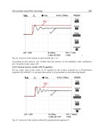
Fig. 3. Received levels on the 32 time-based beam-formed beams of a Ø4m-32-sensor-
antenna for sea state 1, 3 and 6 (left to right) and three passive-active whale types of
orientation: from top to bottom: whale angle of view is near beam aspect, and tail-aspect
(see text). Array DI is 12 dB (see text). The simulated silent whale is at 330° azimuth, 100 m
depth, 1100 m horizontal distance from the buoy. The cumulated plot results from a 25-s
period with 8 whales clicking at depth (see text). Total number of clicks was 189. Beams are
altered by the direct and reverberated paths from the vocal whales’ clicks directly to the
buoy (90 dB and over).
Localising Cetacean Sounds for the
Real-Time Mitigation and Long-Term Acoustic Monitoring of Noise

555
3. Matched filtering using pre-localized sources could raise the SNR in cases when sea-
state and the resulting greater noise levels and reverberations alter the detection rates.
However, as clicks are highly directional, matched filtering in the case of sperm whales
may not always perform as expected as both source signal and reverberated replicas
tend to differ when the source heading changes. As seen in the previous section on click
time–frequency characteristics, both time and frequency contents are angle-dependent.
As this angle is random to the receiver in most cases, the hypothesis of a deterministic
signal is not fulfilled and thus matched filtering would not be optimal. It is also likely
that matched filtering would be less efficient at greater ranges, where signals are more
distorted. According to Daziens (2004), sperm whale clicks matched filtering was
indeed outperformed by an energy detector for ranges greater than 3000 m. In fact, the
latter outperformed matched filtering only for sperm whale click detection. Detection
ranges were then nearly doubled as compared to matched filtering, for the same source

level, detection and false-alarm probabilities, of 50% and 1% respectively. In our case, as
the two-way propagation (source to silent whale to receiver) results in greater
attenuation and distortion than those resulting from a one-way propagation of the same
distance, it is expected that the energy detector will outperform matched filtering.


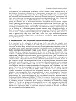
Fig. 4. Statistical plot of the simulated received RMS levels of clicks reflected on a silent
whale located at 1000m distance from the buoy (see text for details on simulation settings).
Ordinates represent the median number of contributing clicks per simulation drawn from
200 simulations (each simulation includes 8 vocal whales clicking once). Also plotted are
lines at the lower quartile and upper quartile values. The whiskers are lines extending from
each end of the box to show the extent of the rest of the data. Outliers are data with values
beyond the ends of the whiskers. Notches over and below median values are medians’ 95%
confidence intervals. Sea-states 0 to 3 and above noise levels in the 1-30 kHz bandwidth are
represented (calculated from Urick, 1996).
Advances in Sound Localization

556
4. In view of the above, which advises a simplistic preprocessing method based on beam-
forming and signal energy, we plotted the received signal intensity distributions from
25 ms time-intervals in Figure 4 (no background noise, no beam-forming) and Figure 5
(with background noise and beam-forming). Figure 4 shows that the resulting
probability density function is bimodal, where the low-level mode represents the click
energy reverberated from the silent whale, and the high-level mode, centred above 120
dB, stems from the click direct, surface and bottom reflected energy at the receiver. We
anticipate that simultaneous occurrence of these two modes on a limited number of
beams could prove robust for a decision stage.


Fig. 5. Distribution of direct, surface, bottom-reflected and silent-whale reverberated clicks.

The top figure is the level-expanded version of Figure 4, which highlights the bimodal
aspect of the received level distribution. The bottom figure represents the resulting
distribution at sea-state 1 with an omni-directional receiver. The same results are obtained
on one beam for sea-state 3 after beam-forming with the antenna described in the text.
Localising Cetacean Sounds for the
Real-Time Mitigation and Long-Term Acoustic Monitoring of Noise

557
4. Space–time and hybrid algorithms for the passive acoustic localisation of
sperm whales and vessels
The prominent approach, described in the previous section, for the passive acoustic
localisation of cetaceans is based on the estimation and spatial inversion of time differences
of arrival of an emitted signal at spatially dispersed sensors, which form an array. A second
class of methods, space–time methods, originated from underwater applications such as
sonar and found valuable applications in other fields such as the analysis of seismic waves
or digital communications. In the latter, a significant amount of research has been devoted
to space–time methods leading to powerful developments over the last 20 years. This
approach has indeed shown to provide more accurate results than TDOA-based methods
(Krim & Viberg, 1996). By maximising the mutual information between the source signal
and array out- put, space–time methods achieve reduced variance in position estimates.
Furthermore they offer simple means for the localisation of multiple simultaneously
radiating sources. While the case of narrowband signals is well documented, the application
of space–time methods to broadband signals, such as those emitted by sperm whales, only
recently found satisfying developments in terms of complexity and accuracy (Dmochowski
et al., 2007). These broadband developments could be imported and largely benefit the
localisation of cetaceans: they indeed outperform TDOA-based methods even with a similar
small number of sensors, a performance, which increases in harsher conditions with high
levels of noise and reverberation. It is not the intention of this paper to thoroughly compare
TDOA-based and space–time methods: this is an evaluation, which requires fairness and
constant updates. Rather, this paper aims to illustrate the interest of developing an

alternative frame concerning localisation, which may be well suited for certain array
configurations. It will present the newly developed and challenging principles behind these
methods and the results they can achieve for the passive acoustic localisation of multiple
sperm whales and vessels. The principles which underlie the increased robustness of space–
time methods will be recalled, and remarks are made concerning other interesting results
which can be obtained via these methods such as broadband beam pattern estimation and
dynamic estimation of attenuation factors. The full description of the approach can be found
at Houégnigan et al., 2010.
A promising new class of hybrid localisers is introduced and its abilities for the localisation
of sperm whales are shown. An important achievement of these hybrid localisers, in the case
of compact arrays, is the reduction of the necessary processing time for results equivalent to
those obtained for space–time methods. All of the developments to follow are intended to be
included in a real-time developed at the Laboratory of Applied Bioacoustics (LAB) of the
Technical University of Catalonia, for the passive monitoring of cetaceans from deep-sea
observatories ().
4.1 General frame of the technical developments
Propagation Model
In this paper a compact array and real far-field sources are under consideration, far beyond
the Rayleigh limit (Ziomek, 1995). The main focus is on the quality of bearing estimation
provided by space-time methods and hybrid methods rather than on their range estimation
capabilities, even though high-resolution space-time estimates of range could be obtained
under certain conditions (Dmochowski et al., 2007). The model moreover focuses on
Advances in Sound Localization

558
broadband sound, hence throughout this paper when reference is made to “cetaceans” this
actually only refers to cetaceans producing broadband sound; note that the developments
are valid for all types of broadband sounds, which includes some vessel sounds.
A three-dimensional array of M sensors is assumed. Due to propagation, each sensor
receives attenuated, phased and noisy versions of the signal s emitted by a cetacean at

spherical position r
s
= [r
s
Ө
s
Фs]. The coordinates of r
s
respectively represent range, azimuth
and elevation.
The signal x
i
(t) received at the i
th
sensor at instant t is modelled as:

(
)
,
() () () ()
ii ji i
ss
xt r st r vt
ατ
=⋅− +, (1.1)
where v
i
represents the additive noise at sensor i, which may include background and
propagation noise, reverberation, and electronic noise. If sensor j is taken as the reference
sensor, the i

th
signal can be expressed by using the propagation delay
,
()
ji
s
r
τ
which is
related to the path difference between the signals received at sensors j and i. Each
i
x is thus
modelled as a noise-corrupted phased and attenuated by distance (term
()
i
s
r
α
) and version
of the signal
s emitted by the cetacean or broadband sound source.
4.2 Methods for the localisation of cetaceans
Methods based on Time Differences of Arrival (TDOA)
To understand the hybrid methods presented below, it is necessary to understand some
aspects of TDOA-based methods (see section 3), but also to compare them to space-time
methods.
The basic principle behind TDOA-based methods is that the time differences of arrival
between the signals received at each sensor are related to the propagation path and the
position of the estimated source. Hence TDOA-based methods feature two main steps:
firstly time-delay estimation (TDE), and secondly a time-space inversion which consists in

forming the position of the radiating source from the group of estimated TDOA related to
the array geometry.

Limits of TDOA-based methods
The estimated time-delays between two noisy signals are themselves corrupted with
broadband noise. Generalised Cross Correlation can improve estimation but this may not be
sufficient. Each of the noisy estimates is then used in a time-space inversion phase and
participates in the construction of a location estimate strongly affected by noise. This is a
severe a priori hindrance that causes anomalies and high variance in the localisation results
even if sophisticated statistical post-processing is applied. Combining all the sensors at
disposal and not using only pairs could yield a strong noise reduction: space-time and
hybrid methods precisely carry out such a beneficial processing. Indeed, the distinction
between the spatial propagation of the signal emitted by cetaceans as opposed to the
supposedly incoherent nature of noise offers powerful means of spatial separation.
Space-time methods
Several space-time methods were implemented for the localisation of cetaceans. The space-
time terminology covers beamformers, spatial spectral estimators, and more generally
methods based on the processing of a spatial observation vector estimated at various time
Localising Cetacean Sounds for the
Real-Time Mitigation and Long-Term Acoustic Monitoring of Noise

559
instants. Space-time methods construct a spatial spectrum by virtually steering the array in
various directions and estimating the received power (in some cases only a power-like index
is estimated). When steered in the direction of a source the power received by the array and
the signal-to-noise ratio will be maximised, and hence the spectrum will exhibit a high peak,
whereas in directions where no sound or only low-power incoherent noise is radiated the
received power will be weak and therefore the spatial spectrum will be relatively flat.
Another way to interpret space-time methods and in particular spatial spectral estimators is
to link them to frequency estimation; indeed these methods do extract information

concerning a spatial frequency: the wavenumber. There exists a strong theoretical link
between spatial frequency estimation and the more familiar temporal frequency estimation
to the point that many methods moved from one domain to the other over the last decades
(Johnson, 1982).
Power estimation
A power
(,)
kk
P
θ
φ
is received when the array is steered in the direction(,)
kk
θ
φ
. Steering is
concretely achieved by delaying each signal according to the theoretical delays observed at
each sensor for a waveform coming from direction
(,)
kk
θ
φ
. One sensor is to be chosen as
reference.
Hence when only one source is present its estimated bearing
(,)
SS
θ
φ



is given by:

(
)
, ar
g
max ( , )
SS kk
k
P
θ
φθφ
=


(2.2)
Multiple sources can be located by searching for multiple peaks in the spatial spectrum. The
accuracy and resolution of the spatial spectrum is related to the way the calculation of power is
carried out. In this paper, the general frame for power calculation is based on the estimation of
a spatial correlation matrix and on various spatial estimators, which function as spatial filters.
Derivation of the spatial correlation matrix
The spatial correlation matrix (SCM) carries information about the correlation between the
signals received at the sensors and the phase and amplitude differences between them.
Other names may be encountered in literature such as space-time covariance matrix, spatio-
spectral correlation matrix or spectro-temporal covariance matrix, but the same spatial
second order statistics is always meant.
The SCM noted as
ℜ
is defined by:

{
}
H
Exxℜ= , (2.3)
where
{
}
E denotes mathematical expectation and where H indicates Hermitian
conjugation.
In practice the signals’ finite nature only permits an estimation of
ℜ
. Estimation is made
more difficult by short duration signals like some of those emitted by cetaceans. In a discrete
frame, the most widely used estimate of
ℜ

can be expressed as:

1
1
S
N
H
nn
n
S
zz
N
=

ℜ=
∑

, (2.4)
Advances in Sound Localization

560
where
S
N is the number of samples corresponding to the signal, where
n
z is a spatial
observation vector at instant n.
ℜ

should not be confused with the cross-correlation function
ij
xx
R as presented in section
(2.1.2), this will be important for the hybrid methods presented in 2.3.
At instant n, i.e. for the n
th
sample acquired by the array, the observation vector is given by

n
z = [
1
()xn
2
()xn … ()

M
xn]
T
, (2.5).
Derivation of the steered spatial correlation matrix
The steered spatial correlation matrix
(,)
kk
θ
φ
ℜ

is the spatial correlation matrix associated
with the array when it is virtually steered in the direction (,)
kk
θ
φ
to estimate the power
received by the array from that particular direction. Steering in the direction (,)
kk
θ
φ
is done
by adequately delaying the received signals with regard to a chosen reference sensor. The
observation vector
n
z then transforms to
()k
n
z

and
(,)
kk
θ
φ
ℜ

can then be expressed as :

()()
1
1
(,)
S
N
kk
H
kk nn
n
S
zz
N
θφ
=
ℜ=
∑

, (2.6)
For example if the j
th

sensor is chosen as a reference, the expression of
()k
n
z is given by:

()k
n
z = [
()
1
1
()
k
j
xn
δ
−
()
2
2
()
k
j
xn
δ
− …
()
()
k
M

j
M
xn
δ
− ]
T
, (2.7)
where
()k
j
m
δ
represents the theoretical delay in samples between the signals at the j
th
and m
th

sensor for a far field source radiating from direction
(,)
kk
θ
φ
. Note that this process may
suffer slight limitations from the sampling frequency since the computable delay in samples
and the actual delay for direction
(,)
kk
θ
φ
do not exactly match.

Spal Spectral
Estimator
Power estimate
Theoretical
Spectral
resolution and
accuracy
Computation
time
Steered Response
Power (SRP or
Bartlett)
(,) (,)
T
kk kk
Pw w
θφ θφ
=
⋅ℜ ⋅


+
(lowest)
+
(shortest)
Capon
(Minimum Variance)
[15]
()

1
1
(,)
(,)
kk
T
kk
P
ww
θφ
θφ
−
=
⋅
ℜ⋅


++ ++
Eigenvalue
decomposition (EIG)
max
(,) (,)
kk kk
P
θ
φλθφ
=
+++ +++
MuSiC
[14]

(,)
1
(,)
kk
kk
T
P
ww
θφ
θφ
=
⋅
Π⋅


++++
(highest)
++++
(longest)
Other estimators:
ESPRIT, Root-MusiC
Propagator…[16]
… … …
Table 1. Description of a few spatial spectral estimators
Localising Cetacean Sounds for the
Real-Time Mitigation and Long-Term Acoustic Monitoring of Noise

561
where
1

[1 1 1 ]
mM
w = ,
max
(,)
kk
λ
θφ
denotes the maximum eigenvalue of ( , )
kk
θ
φ
ℜ

, and
(,)
kk
θ
φ
Π

denotes the noise subspace of ( , )
kk
θ
φ
ℜ

.
Based on the matrix defined in (2.6) we present in table 1 various spatial spectral estimators
used to obtain our results (see below). EIG, Capon, and MuSiC are often referred to as high-

resolution algorithms, and MuSiC is also labelled as subspace-based.
Hybrid spatial spectral estimation
The newly defined and developed hybrid methods are composed of three steps related both
to space-time methods and TDOA-based methods.
Step 1: Calculation of the generalised cross-correlation for all pairs of sensors

Note that using other functions than GCC at this step may bring other interesting results.
Step 2: Construction of a Steered hybrid SCM
(,)
h
y
bkk
θ
φ
ℜ

based on the generalised cross-
correlation functions.
There exists a clear mathematical relationship between the cross correlation and the hybrid
SCM such that the element
i
j
r

on the i
th
line and j
th
column of ( , )
h

y
bkk
θ
φ
ℜ

is given by:

()
()
ij
k
ij x x
ij
rR
δ
=


, (2.8)
i
j
xx
R

represents the estimated generalised cross-correlation function between the signals at
the i
th
and j
th

sensor. The use of
()k
i
j
δ
follows from Eq. (2.7). The operation in Eq (2.8) selects
realisable delays within the cross-correlation functions and repositions the temporal second-
order statistics in a spatial frame.
Step 3: Space-time power estimation

Space-time power estimation can be conducted based on the steered hybrid covariance
matrix ( , )
h
y
bkk
θ
φ
ℜ

. The power estimators presented in table (2.2) can be re-used simply by
replacing ( , )
kk
θ
φ
ℜ

by ( , )
h
y
bkk

θ
φ
ℜ

.
Nomenclature of hybrid methods
The name of a hybrid method will be composed of two parts: firstly the type of spatial
power estimator used and secondly the type of GCC filter used. For example, SRP-SCOT
corresponds to a SCOT filter applied to the Cross-Correlation function at step 1 and a
Steered Response Power at step 3. Similarly MuSiC-ROTH corresponds to a ROTH filter
applied to the Cross-Correlation function in the first phase and a MuSiC Power Estimation
in the third phase. When no filtering is done, a standard Cross-Correlation function is used
and the hybrid method is almost equivalent to the corresponding space-time method except
that the estimated SCM remains hybrid with regard to its construction. In that case we
would write for example SRP-hybrid or MuSiC-hybrid to differentiate them from the
classical space-time SRP and MuSiC. In the case presented here hybridisation typically
consists in going from a temporal second order statistics to a spatio-temporal second-order
statistics.
Note that some methods developed by other authors are very close to the class of hybrid
methods. This is notably the case of the SRP-PHAT algorithm developed by Griebel and
Brandstein (2001). Developed mostly for conference settings with high reverberation it uses
firstly the generalised cross-correlation with a PHAT filter and secondly a steered response
Advances in Sound Localization

562
power approach to localise speakers. However the method is obviously derived in a
different manner and its authors class it as TDOA-based (DiBiase et al., 2001). Indeed, it
does not rely on steered correlation matrices, which would have permitted to relate the
spatial and temporal second order statistics and which would formally place their estimator
in the hybrid group. To our knowledge, the first technical equivalent of a hybrid method

was presented by Dmochowski et al, in 2007, who introduced the parameterised spatial
correlation matrix, a powerful framework which inspired the hybrid steered SCM.
Final methodical remarks
The space-time and hybrid approaches presented here are well suited for far-field cetacean
localisation and in particular for broadband cetacean sound. Typically a relatively small
number of widely spaced sensors are featured while some cetaceans emit sound with a
proportionately high frequency content, which may yield spatial aliasing. Spatial aliasing is
a well known but poorly studied phenomenon caused by the relation between the aperture
of the array and the wavelengths present in the signal.
The philosophy behind the methods presented here is, as in most TDOA-based methods, to
treat the broadband signals received as truly broadband, and not as an artificial composition
of narrowband components. This permits to gain accuracy, to mitigate the effects of spatial
aliasing and to reduce processing time. In order to implement this time approach for
broadband cetacean sound, a simple time-derived spatial correlation matrix is computed.
Sophisticated frequency derivations of the SCM (Wang & Kaveh, 1985) do exist but they
may have difficulties in coping with real-time requirements. Furthermore, given the spatial
dimensions of most arrays deployed underwater, the frequency approach is likely to be
heavily corrupted by spatial aliasing, which will then affect the accuracy of cetaceans’
localisation.
A Short Presentation of the datasets and material
In the frame of the NEMO collaboration (Neutrino Mediterranean Observatory) for neutrino
detection (Riccobene, 2009), more than 2000 hours of multichannel recordings were gathered.
An underwater station was installed 25 km East of the port of Catania (Sicily) at approximately
2000 m depth. The station was equipped with four hydrophones working in a frequency
band, which is sufficiently large (from 36 Hz to 43 kHz) for the detection, classification and
localisation of vocalising cetaceans. The average distance between the sensors was 2.5m. Data
was acquired at a sampling rate of 96 kHz. Vocalising sperm whales were detected with an
algorithm for the real-time detection of impulsive sounds, which provided an estimation of the
onsets and offsets of the sperm whale clicks (Zaugg et al, 2010).
Information from these datasets was extracted to estimate the beampattern and to perform

localisation. The calculations were run under Matlab on a desktop with a 2.8 Ghz Pentium
IV with limited memory which explains some relatively high calculation (Houégnigan et al,
2010).
4.3 Results
Determination of the beam pattern of the array
The beam pattern represents the variation of intensity or sound pressure level received as
the direction of arrival varies, range being fixed. This is valuable information concerning the
capability of the array to localise sources. The beam patterns presented in figures 6.1 and 6.2,
Localising Cetacean Sounds for the
Real-Time Mitigation and Long-Term Acoustic Monitoring of Noise

563
respectively based on SRP and EIG, demonstrate that the array possesses good spatial
separation capabilities with regard to bearing even with only four sensors and is not
strongly affected by sidelobes, grating lobes and aliasing. A broadband sperm whale click of
average energy was selected from the available data sets as a representative reference
source. The traces and maxima, in the beampatterns 6.1 (left) and, even more clearly, in 6.1
(right), are related to the power received by the array. This power is itself related to the path
difference between the sensors for a particular angular position of the source. The simplest
maxima, yet not the most obvious, occurs at the borders of the spectra when the elevation is
at 0º or 180º, i.e. when the source is pointing towards the array from above or from below.
This position minimizes the path difference between three hydrophones (i.e. those with
cartesian coordinate z=0 in the tetrahedron) and maximizes the power received by the
whole array. Given the regular form of the array (the array is almost tetrahedral in shape
but not exactly) it is clear that the power received will be invariant by rotation or by certain
movements. This is verified by the six other maxima, which can be found in the pattern.
There is a clear symmetry among them due to the choice of an azimuth varying from 360º
and not just 180º. In the same way, traces can be explained by considering the array
geometry and how the DOA of the source influences the path difference and power
received. The 9 traces observed (6 traces appear at constant azimuth and 3 traces oscillate

with azimuth in a manner reminiscent of a sine wave) show us that certain positions of the
source create invariance of the power received, this power being relatively high. In these
cases only the power received between pairs of hydrophones is actually maximized and
thus only the path difference between pairs of hydrophones is minimized. There are clearly
more ways of maximizing the power received for pairs than for triplets of sensors and this
explains the extension of the traces and their number. On the whole, the traces observed are
strongly dependent on the array geometry in the sense that they follow all the spatial
positions, which maximize the power received (or minimize the path difference) in pairs of
sensors. With EIG, spectral lines appear much sharper and spatial regions are much more
clearly separated in terms of power than with SRP. For localisation, this implies less
ambiguity in the estimation through clearer and narrower peaks.


Fig. 6.1. Broadband beam pattern for a broadband click computed through SRP (left);
broadband beam pattern for a broadband click, computed through EIG (right). Colour scale
indicates average output power in dB.

Advances in Sound Localization

564
Click-by-click localisation
Click-by-click localisation assumes that each click in a sequence contains information
concerning the position of a vocalising sperm whale. Hence applying various spatial
spectral estimators to a unique click can give an indication concerning their performance.
Among the numerous 5 minutes duration datasets at disposal, the dataset recorded on 14
th

August 2005 from 3pm to 3.05pm was chosen. In this short sequence 819 impulsive sounds
were detected and classified as sperm whale clicks. The localisation procedure was run for
the methods presented above. In order to compare the localisation capabilities of those

methods a single click of average energy, the 40
th
in the sequence, was selected. The
processing of this click was also used to assess processing time. This will permit to decide on
the choice of a suitable algorithm for real-time tracking.
Via Space-time methods
Figure 6.2 present the spatial distribution of power received for the selected click for space-
time methods. A one-degree resolution was used for the computation of the spectra. There is a
clear similarity between them, with spectral lobes, which are characteristic of the array, the
strongest of which should converge towards the putative source location. The located source
appears without ambiguity as a sharp peak within a dense zone of high power in figures 6.2
(left) and 6.2 (right), respectively for the SRP and EIG algorithms. The spatial spectra for
MuSiC and Capon are not presented here since they provided inconsistent location estimates.
The Capon spatial spectrum appeared extremely noisy with many secondary peaks while the
MuSiC spectrum was obviously less noisy but did not have a clear unique peak. The circles,
which appear in 6.2 and 6.3 are artefacts in the construction of the spatial spectrum. Spectral
lines other than circles are actually observed in different positions of the spectrum when the
source is at a different position. However, these artefacts are not appearing randomly: in the
same way as for the beam pattern, spectral lines appear in correlation with the position of the
source and the geometry of the array. This is comparable to frequency estimation where the
spacing between the sampling points (sampling rate) constraints the spectrum as much as the
spectral content of the signal. Here, the placement of the sensors in the array operates a
sampling of space, which has an influence on the spatial spectrum.


Fig. 6.2. Localisation of a broadband click computed with SRP (left); localisation of a
broadband click computed with eigenanalysis spatial spectral estimation (right). Estimated
position:
()
{}

, 176º,74º
ss
θφ
=


. Color scale indicates average output power in dB.
Localising Cetacean Sounds for the
Real-Time Mitigation and Long-Term Acoustic Monitoring of Noise

565
Via Hybrid methods
Figure 6.3 and 6.4 present the spatial distribution of power received for the selected click for
the hybrid methods, which were implemented. A one-degree resolution was used for the
computation of the spectra. In figure 3.7 a side view of the spatial spectra (corresponding to
elevation against power) is shown which permits to evaluate the number of side lobes, the
separation between signal and noise for hybrid MuSiC and to visualise a narrow localisation
peak, which is not obvious from 3.6. There is clearly a similarity between the hybrid spectra
and the spectra obtained with space-time methods.



Fig. 6.3. Performance of SRP-ROTH (left); performance of MUSIC-SCOT (right), colour scale
indicates average output power in dB.



Fig. 6.4. Performance of MUSIC-SCOT, (elevation only), colour scale indicates average
output power in dB.
Advances in Sound Localization

566
The located source appears clearly as a sharp peak within the red-coloured zone in figure
6.3, respectively for SRP-ROTH and MuSiC-SCOT. The hybrid EIG algorithm failed to give
results, which could compare with its non-hybrid version, it featured large spectral lines of
high power which could not correspond to a real scenario and therefore it is not included
here. The performance achieved by SRP-ROTH was very similar to that obtained for the
non-hybrid EIG, with a reduced processing time (Houégnigan et al, 2010). With SRP-SCOT
various high amplitude secondary peaks appeared which was not the case was for SRP-
ROTH.
The Capon and Music methods did seem to perform more reliably when hybridised. They
could isolate a main peak, which reduced ambiguity as figure 6.4 shows for MuSiC-SCOT.
MuSiC-SCOT and MuSiC-ROTH in particular did achieve a powerful separation of signal
(peak) and noise (lower power zones) as could be expected from the (non-hybrid) theory of
MuSiC (Schmidt, 1986). The localisation obtained for the hybridised versions of Capon
permitted to achieve a consistent localisation but figures are not presented for conciseness.
Several secondary peaks appeared for Capon-SCOT but they were not yet problematic; they
were not present for Capon-ROTH. In general ROTH hybrids seemed to provide the most
reliable localisations.
Tracking of sperm whales and boats
Repeating the localisation procedure for each of the impulsive sounds detected in a 5-
minute window allowed to track the movement of emitting sources classified as sperm
whales or boats.
Track 1: Dataset 18
th
August 2005, 10 pm
Besides some isolated locations, which may be anomalies or simply scarcely vocalising
sperm whales, two main tracks can be isolated with a clear separation in azimuth and
elevation against time. The first one is found close to (θ
1

, φ
1
) = {160°, 60°} and the second one
close to (θ
2
, φ
2
) = {200°, 55°}.


Fig. 6.5. Sperm whale tracking, 18
th
August 2005, 10pm
Track 2: Dataset 09
th
August 2005, 09 pm
776 sperm whale clicks were taken into account for localisation. There are two main clusters
of points with sound sources moving around (θ
1
,φ
1
)={80°,50°} and (θ
2
,φ
2
)={290°,30°} and
some more isolated clicks. The second cluster may contain several closely spaced animals
but on the whole at least two vocalising mammals can be numbered in this sequence. The
mammal corresponding to the first cluster has a very clear pattern of decreasing elevation
Localising Cetacean Sounds for the

Real-Time Mitigation and Long-Term Acoustic Monitoring of Noise

567
and azimuth in time. The second cluster is less obvious; there could be two animals close to
each other. Further clustering and disentanglement of click series could be useful to obtain a
better separation. From (c), elevation seems to indicate that there could be more than just
two animals in the second cluster indeed elevation normally varies very little at large
distances whereas well separated values of elevation (>5º) were found at a particular instant
in time. Since the particular geometry makes it also less sensitive to small variation in
azimuth, there could well be more than one animal in that cluster.


Fig. 6.6. Sperm whale tracking, 09
th
August 2005, 09pm
Track 3: Dataset 18
th
August 2005, 11 pm
760 sperm whale clicks were taken into account for localisation. One animal is clearly
localised around (θ
1
, φ
1
) = {110°, 45°} and features a relatively stable elevation and a
decreasing azimuth.


Fig. 6.7. Sperm whale tracking, 18
th
August 2005, 11pm

Track 4: Dataset 09
th
August 2005, 02 am
701 impulsive sounds were taken into account for localisation. An experienced operator
aurally identified them as being shipping impulsive sounds. Contrary to the tracking of
sperm whales, the tracking of boats features a clear evolution of DOA during the available
five minutes. This seems to confirm the fact that boats are localised since their speed is
expected to be much faster than that of sperm whales. The first cluster around (θ
1
, φ
1
) =
{100°, 65°} corresponds to a source which starts to radiate around 150s. It features a slow but
clear increase of both azimuth and elevation. The second cluster around (θ
2
, φ
2
) = {275°, 45°}
corresponds to a source which radiates regularly during the 5 minutes of recording. It
features a fast decrease of azimuth and a fast increase of elevation.
Advances in Sound Localization

568

Fig. 6.8. Vessel tracking, 09
th
August 2005, 02am
4.3 Discussion
Discussion on click-by-click localisation
For space-time methods, two main reasons could explain the poor performance of the Capon

and MuSiC algorithms which theoretically perform better than SRP. Firstly, both of these
methods are extremely sensitive to the possible misestimation of the SCM (Krim & Viberg,
1996). SCM is in particular difficult to estimate correctly for short duration signals. This
problem appeared to be partly solved by hybrid methods. Secondly, these methods are
sensitive to the amplitude mismatch caused by unknown differences in sensitivity of the
hydrophones. This could be corrected for but only at the expense of additional computations,
which are not developed here for conciseness. These corrections would also add to the
respective processing times. Some of the hybrid methods presented in the next section seemed
to demonstrate that this problem could be solved with reasonable processing times.
Among the space-time methods, the SRP algorithm, even though it is less sophisticated,
seems to be the best compromise between accuracy and processing time (Houégnigan et al,
2010). Considering that calculations could be carried out much faster in parallel and on a
dedicated computation platform, considering also commonly observed inter-click intervals
for sperm whales between 0.5 and 2 seconds and the pauses been sequences of clicks
(Wahlberg, 2002), an SRP implementation could be well-suited for real-time applications.
The interest of hybrid methods seems manifest from the results, which can be compared to
those obtained with space-time methods while requiring less processing time. For example,
SRP-ROTH was comparable to the non-hybrid EIG but took about a third of its time. In
general the hybrid methods presented here (many other filters -and thus other hybrids-
could be considered) are also extremely profitable to the simple SRP algorithm. An
interpretation of these results based on the nature of the filters used in the Generalised
Cross-Correlation can be done.
(1) By filtering the signals, hybrids seem to construct a better estimation of the spatial
correlation matrix. This estimate is not necessarily closer to the real spatial correlation
matrix but more likely this estimate is more adapted to the nature of the spatial spectral
estimators to which it is associated. Each of the estimators indeed uses a particular balance
of noise and signal to achieve localisation, which is affected by the filters used for the
Generalised Cross-Correlation.
The bad performance of the hybridised EIG, which relies on signal information by
estimating the highest eigenvalue, is a sign that the signal components obtained after

filtering are incorrect. The SCOT and ROTH filters, by taking into account coherence,
Localising Cetacean Sounds for the
Real-Time Mitigation and Long-Term Acoustic Monitoring of Noise

569
blindly enhance spectral regions with high energy which may contain both noise and signal.
The signal estimated by EIG-SCOT or EIG-ROTH is hence probably not only signal but a
mixture of signal and noise, which leads to localisation errors. A filter more adapted to that
algorithm could be imagined. On the contrary, since MuSiC and Capon rely on noise
estimation, they location estimation is improved. Obviously, even though some noisy
components are labelled as signal, the remaining noise components, those with low energy,
are likely to contain less signal and hence to improve MuSiC and Capon.
(2) The filters have to be well adapted to the ambient noise present and to the levels of
reverberation. It was for example noticed that the PHAT filter, frequently used for human
speaker localisation was not well suited for data from the NEMO deep-sea observatory.
More adaptive pre-filters could also be created. In general, in the use of hybrids one should
be aware of the effects of each filter and of the modus operandi of each spectral estimator
with regard to the spatial correlation matrix.
(3) The signals received on hydrophones resulting from broadband sound emitted by
cetaceans are corrupted by noise and may feature an important dynamic range across the
frequency bands, which makes estimation more difficult. Indeed, the contribution of weak
signal components is likely to be underestimated whereas they could provide valuable
information. Pre-whitening can reduce this dynamic range and is one of the capabilities of
the SCOT and ROTH filters.
4.4 Discussion on tracking
Although they cannot be confirmed by sightings, the estimated tracks were consistent with
what can be expected from a sperm whale. In five-minute sequences the bearing may not
change drastically given the expected slow speed of sperm whales (such as 0.2 to 2.6 m/s
observed in Wahlberg, 2002) but coherent evolution of azimuth and elevation with time can be
reconstructed. Track 6 shows that the localisation of vessels performs consistently without

even proceeding to clustering. For sperm whales, additional clustering may add consistency to
the results displayed but might as well discard valid isolated clicks. Already, the spatial
separation abilities permitted to proceed to an estimation of the minimal number of vocalising
mammals. The developed methods would benefit from being trained on data using a known
moving source; this would permit to assess more precisely their performances.
5. Conclusions
5.1 Ambient noise imaging to track non-vocalising sperm whales
For a given and well-characterized signal, detection probabilities mostly depend on the
background noise level. Before attempting the implementation of our passive approach in a
specific area, it should be noted that ambient noise level statistics are the most limiting
factor. We inferred from the literature that, in the band of interest, noise level was around 90
dB
rms re 1µPa for sea-state 1 and a 1–30 kHz bandwidth. From our simulation results,
energy-based detection thresholds would work until 1000 m. Nonetheless, each increase of 6
dB in background noise level, which is far from unusual, would half the detection range, as
most propagation spreading is spherical in our case, and would make the system unreliable
due to the dependency on weather conditions. Advanced post-processing of the received
low-level signals was not studied. The inherent spatio-temporal nature of sperm whale
acoustics and behaviour requires the use of either stochastic or determinist signal processing
Advances in Sound Localization

570
to further increase the SNR. Statistical methods for ANI have been thoroughly studied in
shallow water (Potter & Chitre, 1996, 1999), but due to the numerous contextual differences,
especially the limited number of active sources, it is likely that a stochastic approach would
not be appropriate in our case. On the other hand, a determinist approach founded on
proper modelling of source angular variability could prove robust. Among other well-
documented methods, passive 3D localization of active sperm whales could then provide
triggering information to coherently sum up the silent whale’s response and increase the
SNR and compensate for the ambient noise variability.

The reported multi-pulse structure of (most probably) offaxis clicks was not simulated, due
to our incapacity to infer a model of its three-dimensional properties. We hence limited our
study to the propagation of the first main pulse. Yet, including this feature would not
impact upon the received levels except in the rare cases of constructive or destructive
overlaps. The greatest impact would more likely be on the ‘fillup’ of the time–space window
with more high-energy pulses at the monitoring point, which may handicap the search for
low level echoes in background noise. It is generally reported that the secondary pulses are
rarely more than two or three and only appear at frequencies higher than 4 to 5 kHz (see
Figure 1). The whole signal duration may then increase to 20 msec which results in a
maximum 20×8×2=320 msec time period. This is one-third of the search time window, for 8
vocal whales and taking direct, surface and bottom reflected signals to the buoy into
account, at a rate of 1click/whale/s.
In the usual case, detection rates would not be drastically altered. This paper would not be
complete without a note on false alarm rates and how they would impact on a vessel’s
decision, as detectable echoes from the surface may often come from different sources, like a
densely concentrated group of fish. At-sea experiments and real recordings may provide the
relevant information to discriminate these other types of objects, e.g. by incorporating their
monitored spatio-temporal and behavioural characteristics. Scattering was only modelled by
surface and bottom reflection coefficients being altered depending on sea-state and bottom
type, respectively. As a result, our scattering model only affects specular rays.
Reverberation, e.g. nonspecular rays back-scattered from surface, bottom or deep scattering
layers was not mentioned nor simulated. When propagating through a deep scattering
layer, direct rays from source to target could also reach the receiver with interference
scattered from the deep layer, attenuated by 40 to 50 dB (Jensen et al., 2000). Such
attenuation could differ when deep scattering layers are at lower depth at night-time.
During daytime, such layers tend to be at greater depths and would be further attenuated
due to propagation loss. In either case, the resulting reverberations may interfere with the
low-level echoes from silent whales. Similarly, modelling of surface and bottom scattering
would provide important information on the interferences from the reverberated sources as
a function of sea-state and time, since no detection will be possible if these are omnipresent,

even for low scattering strengths. Even though we have shown that signals echoed from
silent whales could be detectable at only low sea-states, when surface scattering may
become negligible, bottom scattering strength could constantly interfere with and increase
noise to critical levels. In this work, simulations accounted for a given number of vocalizing
whales, each producing one direct, one surface reflected and one bottom-reflected ray to the
receiver and to one silent whale, which in turn radiated the corresponding echoes modelled
by one direct, one surface-reflected and one bottom-reflected ray to the receiver. In fact,
these 12 resulting rays represent only one part of the real signal at the receiver, as all
vocalizing whales would also scatter energy from other whales’ clicks. In addition,
Localising Cetacean Sounds for the
Real-Time Mitigation and Long-Term Acoustic Monitoring of Noise

571
simulations were limited to allow only one bottom and one surface reflection. Multiple
reflections from vocalizing whales’ clicks would originate weak signals of a similar order of
magnitude as the simulated silent whale’s echoes and should be discarded as well. So far,
we have not studied how adding these additional scatterers and pathways could alter the
current results, as the objective of this work was to study whether a signal excess from a
silent whale near the surface could be measured. The raised ambiguity and false-alarm rates
due to unpredicted and more complex pathways would probably call for a more advanced
detector. As the primary task of the WACS is to localize active whales using an array of
receivers, the resulting information could be used to perform forward modelling of the
arrival structure, and then to compare this with observations to identify the anticipated
replica arrivals. Echoed signals from silent whales could then be detected by a band-limited
energy detector. In future work the authors hope to be able to simulate the same scenario
with an unlimited number of reflections and enable back-scattering from active whales so
that more complex detectors and matched field methods can properly be evaluated.
While this study is restricted to sperm whales, the ANI approach might progressively
extend to wider possibilities, as large baleen whales passing through a wide pod of sperm
whales are also to be detected, probably with higher contrast in the case of species such as

fin and blue whales. Most large baleen whales only produce very low frequency sounds
(most of the energy remains below 100 Hz) that reverberate in a complex way in the SOFAR
channel and mix with all types of low-frequency sources summing up to great sound
pressure levels (Potter & Delory, 1998). As a direct consequence, designing a permanent
solution for passive localization of these whales is a difficult task and furthermore can be
performed only with very wide aperture bottom-mounted arrays. The low and, at times,
negative signal-to-noise ratios at relatively short range from the whales have motivated the
specific development of advanced signal processing algorithms that have not yet been
implemented and still need further development (Delory & Potter, 1999; Delory et al., 1999).
We believe that our approach could be an alternative worth considering in areas where
sperm whale populations are geographically dense and stable over time. Furthermore, this
method would have to be a complementary component of a more complex system like the
previously described WACS in order to be viable and useful.
In conclusion, the results provided quantitative information as regards the implementation
of a passive approach using sperm whale clicks as illuminating sources. Received levels are
centred on ambient noise levels for low sea-states, motivating the use of beam-forming to
raise signal levels and extract bearing information. Validation of the method introduced in
this paper is essential before advanced signal enhancement techniques can be properly
evaluated, leading to the prior necessity of performing experiments in the field. From a
broader perspective, as permanent passive techniques based on natural acoustic energy
would be probably less costly and less prejudicial to cetaceans than conventional active
solutions the authors believe that they merit further investigation.
5.2 Space–time and hybrid algorithms for the passive acoustic localisation of sperm
whales and vessels
This paper presented space-time estimators in a broadband frame and introduced novel
hybrid methods. These developments could benefit the localisation of cetaceans emitting
broadband sound, e.g. sperm whales, and can also be used for the localisation of vessels
emitting broadband sound. When hybridised, basic space-time algorithms such as SRP were
improved and performed as consistently as more sophisticated high-resolution estimators