Advances in Vibration Analysis Research Part 7 ppt
Bạn đang xem bản rút gọn của tài liệu. Xem và tải ngay bản đầy đủ của tài liệu tại đây (619.75 KB, 30 trang )
Dynamic Analysis of a Spinning Laminated
Composite-Material Shaft Using the hp-version of the Finite Element Method
169
[]
{}
() ( )
[]
{}
() ( )
[]
{}
() ( )
{}
() ( )
{}
() ( )
{}
() ( )
0
1
0
1
0
1
1
1
1
U
V
W
x
xx
y
yy
p
UU m m
m
p
VV m m
m
p
WW m m
m
p
xxmm
m
p
yymm
m
p
mm
m
UNq xtf
VNq ytf
WNq ztf
Nq tf
Nq tf
Nq tf
β
β
φ
ββ
ββ
φφ
ξ
ξ
ξ
β
βξ
β
βξ
φφξ
=
=
=
=
=
=
⎧
==⋅
⎪
⎪
⎪
⎪
==⋅
⎪
⎪
⎪
==⋅
⎪
⎪
⎨
⎪
⎡⎤
==⋅
⎣⎦
⎪
⎪
⎪
⎡⎤
⎪
==⋅
⎣⎦
⎪
⎪
⎪
⎡⎤
==⋅
⎪
⎣⎦
⎩
∑
∑
∑
∑
∑
∑
(12)
where [
N] is the matrix of the shape functions, given by
,, , , , 1 2 , , , , ,
xy UVW
xy
UVW p p p p p p
Nfff
ββφ
ββφ
⎡
⎤
⎡⎤
=
⎢
⎥
⎣⎦
⎣
⎦
…… (13)
where
,, , ,
xy
UVW
p
pp p p
β
β
and
p
φ
are the numbers of hierarchical terms of
displacements (are the numbers of shape functions of displacements). In this work,
xy
UVW
p
pp p p pp
ββφ
== = = ==
The vector of generalized coordinates given by
{}
{
}
,, , , ,
xy
T
UVW
qqqqqqq
ββφ
= (14)
where
{}
{}
(){}
{}
()
{
{}
{}
()
{}
{}
()
{}
{}
()
{}
{}
()
123
123
123 123
123
12 3
, , , , exp ; , , , , exp ;
, , , , exp ; , , , , exp ;
, , , , exp ; , , , , exp
U V
Wx p
x
yp
y
TT
UpV p
T
T
Wp xxxx
T
T
yyy y p
qxxxx jtqyyyy jt
q
zzz
yj
t
qj
t
qjtqjt
β
φ
β
β
βφ
ωω
ωββββω
βββ β ω φφφ φ ω
==
==
⎫
⎪
==
⎬
⎪
⎭
(15)
The group of the shape functions used in this study is given by
()() ()
(
)
}
{
122
1sin,;1,2,3,
rrr
fff rr
ξξ δξδπ
+
=− = = = = (16)
The functions (f
1
, f
2
) are those of the finite element method necessary to describe the nodal
displacements of the element; whereas the trigonometric functions f
r+2
contribute only to the
internal field of displacement and do not affect nodal displacements. The most attractive
particularity of the trigonometric functions is that they offer great numerical stability. The
shaft is modeled by elements called hierarchical finite elements with p shape functions for
Advances in Vibration Analysis Research
170
each element. The assembly of these elements is done by the h- version of the finite element
method.
After modelling the spinning composite shaft using the hp- version of the finite element
method and applying the Euler-Lagrange equations, the motion’s equations of free vibration
of spinning flexible shaft can be obtained.
[]
{}
[]
{}
[]
{}
{}
0
p
Mq G C q Kq
⎡⎤
⎡⎤
++ + =
⎣⎦
⎣⎦
(17)
[M] and [K] are the mass and stiffness matrix respectively, [G] is the gyroscopic matrix and
[C
p
] is the damping matrix of the bearing (the different matrices of the equation (17) are
given in the appendix).
3. Results
A program based on the formulation proposed to resolve the resolution of the equation (17).
3.1 Convergence
First, the mechanical properties of boron-epoxy are listed in table 1, and the geometric
parameters are L =2.47 m, D =12.69 cm, e =1.321 mm, 10 layers of equal thickness (90°, 45°,-
45°,0°
6
, 90°). The shear correction factor k
s
=0.503 and the rotating speed Ω =0. In this
example, the boron -epoxy spinning shaft is modeled by one element of length L, then by
two elements of equal length L/2.
Graphite-epoxy Boron-epoxy
E
11
(GPa)
E
22
(GPa)
G
12
(GPa)
G
23
(GPa)
ν
12
ρ (kg/m
3
)
139.0
11.0
6.05
3.78
0.313
1578.0
211.0
24.1
6.9
6.9
0.36
1967.0
Table 1. Properties of composite materials (Bert & Kim, 1995a)
The results of the five bending modes for various boundary conditions of the composite
shaft as a function of the number of hierarchical terms p are shown in figure 12. Figure
clearly shows that rapid convergence from above to the exact values occurs when the
number of hierarchical terms increased. The bending modes are the same for a number of
hierarchical finite elements, equal 1 then 2. This shows the exactitude of the method even
with one element and a reduced number of the shape functions. It is noticeable in the case of
low frequencies, a very small p is needed (p=4 sufficient), whereas in the case of the high
frequencies, and in order to have a good convergence, p should be increased.
3.2 Validation
In the following example, the critical speeds of composite shaft are analyzed and compared
with those available in the literature to verify the present model. In this example, the
composite hollow shafts made of boron-epoxy laminae, which are considered by Bert and
Dynamic Analysis of a Spinning Laminated
Composite-Material Shaft Using the hp-version of the Finite Element Method
171
Kim (Bert & Kim, 1995a), are investigated. The properties of material are listed in table1. The
shaft has a total length of 2.47 m. The mean diameter D and the wall thickness of the shaft
are 12.69 cm and 1.321 mm respectively. The lay-up is [90°/45°/-45°/0°
6
/90°] starting from
the inside surface of the hollow shaft. A shear correction factor of 0.503 is also used. The
shaft is modeled by one element. The shaft is simply-supported at the ends. In this
validation, p =10.
0
200
400
600
800
1000
1200
1400
1600
1800
2000
4 5 6 7 8 9 10 11 12
p
ω [Hz]
ω1 (S-S)
ω2 (S-S)
ω3 (S-S)
ω4 (S-S)
ω5 (S-S)
ω1 (C-S)
ω2 (C-S)
ω3 (C-S)
ω4 (C-S)
ω5 (C-S)
ω1 (C-C)
ω2 (C-C)
ω3 (C-C)
ω4 (C-C)
ω5 (C-C)
Fig. 12. Convergence of the frequency ω for the 5 bending modes of the composite shaft for
different boundary conditions (S: simply-supported; C: clamped) as a function of the
number of hierarchical terms p
The result obtained using the present model is shown in table 2 together with those of
referenced papers. As can be seen from the table our results are close to those predicted by
other beam theories. Since in the studied example the wall of the shaft is relatively thin,
models based on shell theories (Kim & Bert, 1993) are expected to yield more accurate
results. In the present example, the critical speed measured from the experiment however is
still underestimated by using the Sander shell theory while overestimated by the Donnell
shallow shell theory. In this case, the result from the present model is compatible to that of
the Continuum based Timoshenko beam theory of M-Y. Chang et al (Chang et al., 2004a). In
this reference the supports are flexible but in our application the supports are rigid.
In our work, the shaft is modeled by one element with two nodes, but in the model of the
reference (Chang et al., 2004a) the shaft is modeled by 20 finite elements of equal length (h-
version). The rapid convergence while taking one element and a reduced number of shape
functions shows the advantage of the method used. One should stress here that the present
model is not only applicable to the thin-walled composite shafts as studied above, but also
to the thick-walled shafts as well as to the solid ones.
Advances in Vibration Analysis Research
172
L=2.47 m, D =12.69 cm, e =1.321 mm, 10 layers of equal thickness (90°, 45°,-45°,0°
6
,90°)
Theory or Method Ω
cr1
(rpm)
Zinberg & Symonds, 1970
Dos Reis et al., 1987
Kim & Bert, 1993
Bert, 1992
Bert & Kim, 1995a
Singh & Gupta, 1996
Chang et al., 2004a
Present
Measured experimentally
EMBT
Bernoulli–Euler beam theory with stiffness
determined by shell finite elements
Sanders shell theory
Donnell shallow shell theory
Bernoulli–Euler beam theory
Bresse–Timoshenko beam theory
EMBT
LBT
Continuum based Timoshenko beam theory
Timoshenko beam theory by the hp- version
of the FEM.
6000
5780
4942
5872
6399
5919
5788
5747
5620
5762
5760
Table 2. The first critical speed of the boron-epoxy composite shaft
The first eigen-frequency of the boron-epoxy spinning shaft calculated by our program in
the stationary case is 96.0594 Hz on rigid supports and 96.0575 Hz on two elastic supports of
stiffness 1740 GN/m. In the reference (Chatelet et al., 2002), they used the shell’s theory for
the same shaft studied in our case and on rigid supports; the frequency is 96 Hz. In this
example, is not noticeable the difference between shaft bi-supported on rigid supports or
elastic supports because the stiffness of the supports are very large.
3.3 Results and interpretations
In this study, the results obtained for various applications are presented. Convergence
towards the exact solutions is studied by increasing the numbers of hierarchical shape
functions for two elements. The influence of the mechanical and geometrical parameters
and the boundary conditions on the eigen-frequencies and the critical speeds of the
embarked spinning composite shafts are studied. In this study, p = 10.
3.3.1 Influence of the gyroscopic effect on the eigen-frequencies
In the following example, the frequencies of a graphite- epoxy spinning shaft are analyzed.
The mechanical properties of shaft are shown in table 1, with k
s
= 0.503. The ply angles in
the various layers and the geometrical properties are the same as those in the first example.
Figure 13 shows the variation of the bending fundamental frequency ω as a function of
rotating speed Ω for different boundary conditions. The gyroscopic effect inherent to
rotating structures induces a precession motion. When the rotating speed increase, the
forward modes (1F) increase, whereas the backward modes (1B) decrease. The gyroscopic
effect causes a coupling of orthogonal displacements to the axis of rotation, and by
consequence separate the frequencies in two branches: backward precession mode and
forward precession mode. In all cases, the forward modes increase with increasing rotating
speed however the backward modes decrease.
Dynamic Analysis of a Spinning Laminated
Composite-Material Shaft Using the hp-version of the Finite Element Method
173
400
500
600
700
800
900
1000
1100
1200
1300
0 20000 40000 60000 80000 100000
Ω [rpm]
ω [rad/s]
1B (S-S)
1F (S-S)
1B (C-C)
1F (C-C)
1B (C-S)
1F (C-S)
1B (C-F)
1F (C-F)
Fig. 13. The first backward (1B) and forward (1F) bending mode of a graphite- epoxy shaft
for different boundary conditions and different rotating speeds (S: simply-supported;
C: clamped; F: free)
0
500
1000
1500
2000
2500
3000
3500
0 10000 20000 30000 40000 50000 60000 70000 80000 90000 100000
Ω [rpm]
ω
[rad/s]
1B (SFS)
1F (SFS)
1B (SSS)
1F (SSS)
1B (CFC)
1F (CFC)
1B (CSC)
1F (CSC)
1B (CSF)
1F (CSF)
1B (SSF)
1F (SSF)
Fig. 14. The first backward (1B) and forward (1F) bending mode of a boron- epoxy shaft for
different boundary conditions and different rotating speeds. L =2.47 m, D =12.69 cm, e =1.321
mm, 10 layers of equal thickness (90°, 45°,-45°,0°
6
, 90°)
Advances in Vibration Analysis Research
174
3.3.2 Influence of the boundary conditions on the eigen-frequencies
In the following example, the boron-epoxy shaft is modeled by two elements of equal length
L/2. The frequencies of the spinning shaft are analyzed. The mechanical properties of shaft
are shown in table 1, with k
s
= 0.503. The ply angles in the various layers and the geometrical
properties are the same as those in the preceding example.
Figure 14 shows the variation of the bending fundamental frequency ω according to the
rotating speeds Ω for various boundary conditions. According to these found results, it is
noticed that, the boundary conditions have a very significant influence on the eigen-
frequencies of a spinning composite shaft. For example, by adding a support to the mid-
span of the spinning shaft, the rigidity of the shaft increases which implies the increase in
the eigen-frequencies.
3.3.3 Influence of the lamination angle on the eigen-frequencies
By considering the same preceding example, the lamination angles have been varied in
order to see their influences on the eigen-frequencies of the spinning composite shaft.
Figure 15 shows the variation of the bending fundamental frequency ω according to the
rotating speeds Ω (Campbell diagram) for various ply angles. According to these results, the
bending frequencies of the composite shaft decrease when the ply angle increases and vice
versa.
200
300
400
500
600
700
800
0 10000 20000 30000 40000 50000 60000 70000 80000 90000 100000
Ω [rpm]
ω
[rad/s]
1B 0°
1F 0°
1B 15°
1F 15°
1B 30°
1F 30°
1B 45°
1F 45°
1B 60°
1F 60°
1B 75°
1F 75°
1B 90°
1F 90°
Fig. 15. The first backward (1B) and forward (1F) bending mode of a boron- epoxy shaft
(S-S) for different lamination angles and different rotating speeds. L =2.47 m, D =12.69 cm,
e =1.321 mm, 10 layers of equal thickness
3.3.4 Influence of the ratios L/D, e/D and η on the critical speeds and rigidity
The intersection point of the line (Ω = ω) with the bending frequency curves (diagram of
Campbell) indicate the speed at which the shaft will vibrate violently (i.e., the critical
speed Ω
cr
).
Dynamic Analysis of a Spinning Laminated
Composite-Material Shaft Using the hp-version of the Finite Element Method
175
In figure 16, the first critical speeds of the graphite-epoxy composite shaft (the properties are
listed in table 1, with k
s
=0.503) are plotted according to the lamination angle for various
ratios L/D and various boundary conditions (S-S, C-C). From figure 16, the first critical speed
of shaft bi-simply supported (S-S) has the maximum value at η = 0° for a ratio L/D = 10, 15
and 20, and at η = 15° for a ratio L/D = 5. For the case of a shaft bi-clamped (C-C), the
maximum critical speed is at η = 0° for a ratio L/D = 20 and at η = 15° for a ratio L/D = 10 and
15, and at η = 30° for a ratio L/D = 5.
Above results can be explained as follows. The bending rigidity reaches maximum at η = 0°
and reduces when the lamination angle increases; in addition, the shear rigidity reaches
maximum at η = 30° and minimum with η = 0° and η = 90°. A situation in which the
bending rigidity effect predominates causes the maximum to be η = 0°. However, as
described by Singh ad Gupta (Singh & Gupta, 1994b), the maximum value shifts toward a
higher lamination angle when the shear rigidity effect increases. Therefore, while comparing
the phenomena of figure 16, the constraint from boundary conditions would raise the
rigidity effect. A similar is observed for short shafts.
0
10000
20000
30000
40000
50000
60000
70000
80000
90000
0 153045607590
η [°]
Ω
1cr
[rpm]
L/D=5; S-S
L/D=10; S-S
L/D=15; S-S
L/D=20; S-S
L/D=5; C-C
L/D=10;C-C
L/D=15; C-C
L/D=20;C-C
Fig. 16. The first critical speed Ω
1cr
of spinning composite shaft according to the lamination
angle η for various ratios L/D and various boundary conditions (S-S, C-C)
In figures 17 and 18, the first critical speeds according to ratio L/D of the same graphite-
epoxy shaft bi-simply supported (S-S) and the same graphite-epoxy shaft bi- clamped (C-C)
for various lamination angles. It is noticeable, if ratio L/D increases, the critical speed
decreases and vice versa.
Advances in Vibration Analysis Research
176
0
10000
20000
30000
40000
50000
60000
5 101520
L/D
Ω
1cr
[rpm]
η=0°
η=15°
η=30°
η=45°
η=60°
η=75°
η=90°
Fig. 17. The first critical speed Ω
1cr
of spinning composite shaft bi- simply supported (S-S)
according to ratio L/D for various lamination angles η
0
10000
20000
30000
40000
50000
60000
70000
80000
90000
5 101520
L/D
Ω
1cr
[rpm]
η=0°
η=15°
η=30°
η=45°
η=60°
η=75°
η=90°
Fig. 18. The first critical speed Ω
1cr
of spinning composite shaft bi- clamped (C-C) according
to ratio L/D for various lamination angles η
Dynamic Analysis of a Spinning Laminated
Composite-Material Shaft Using the hp-version of the Finite Element Method
177
0
2000
4000
6000
8000
10000
12000
0 153045607590
η
[°]
Ω
1cr
[rpm]
e/D=0,02; S-S
e/D=0,04; S-S
e/D=0,06; S-S
e/D=0,08; S-S
e/D=0,02; C-C
e/D=0,04; C-C
e/D=0,06; C-C
e/D=0,08; C-C
Fig. 19. The first critical speed Ω
1cr
of spinning composite shaft according to the lamination
angle η for various ratios e/D and various boundary conditions (S-S, C-C); (L/D = 20)
Figure 19 plots the variation of first critical speeds of the same graphite-epoxy composite
shaft with ratio L/D = 20 according to the lamination angle for various e/D ratios and various
boundary conditions. It is noticed the influence of the e/D ratio on the critical speed is almost
negligible; the curves are almost identical for the various e/D ratios of each boundary
condition. This is due to the deformation of the cross section is negligible, and thus the
critical speed of the thin-walled shaft would approximately independent of thickness ratio
e/D. According to above results, while predicting which stacking sequence of the spinning
composite shaft having the maximum critical speed, we should consider L/D ratio and the
type of the boundary conditions. I.e., the maximum critical speed of a spinning composite
shaft is not forever at ply angle equalizes zero degree, but it depends on the L/D ratio and
the type the boundary conditions.
3.3.5 Influence of the stacking sequence on the eigen-frequencies
In order to show the effects of the stacking sequence on the eigen-frequencies, a spinning
carbon- epoxy shaft is mounted on two rigid supports; the mechanical and geometrical
properties of this shaft are (Singh & Gupta, 1996):
E
11
= 130 GPa, E
22
= 10 GPa, G
12
= G
23
= 7 GPa, ν
12
= 0.25, ρ = 1500 Kg/m
3
L =1.0 m, D = 0.1 m, e = 4 mm, 4 layers of equal thickness, k
s
= 0.503
A four-layered scheme was considered with two layers of 0° and two of 90° fibre angle. The
flexural frequencies have been obtained for different combinations (both symmetric and
unsymmetric) of 0° and 90° orientations (see figure 20). This figure plots the Campbell
diagram of the first eigen-frequency of a spinning shaft for various stacking sequences. It
can be observed from this figure that, for symmetric configurations, the frequency values of
the spinning composite shaft are very close, and do have a slight dependence on the relative
positioning of the 0° and 90° layers.
Advances in Vibration Analysis Research
178
315
320
325
330
335
340
345
350
355
360
365
0 10000 20000 30000 40000 50000 60000 70000 80000 90000 100000
Ω [rpm]
ω
1
[Hz]
1B (90°,90°,0°,0°)
1F (90°,90°,0°,0°)
1B (0°,0°,90°,90°)
1F (0°,0°,90°,90°)
1B (0°,90°,90°,0°)
1F (0°,90°,90°,0°)
1B (90°,0°,0°,90°)
1F (90°,0°,0°,90°)
1B (0°,90°,0°,90°)
1F (0°,90°,0°,90°)
1B (90°,0°,90°,0°)
1F (90°,0°,90°,0°)
Fig. 20. First bending eigen-frequency of the spinning carbon- epoxy shaft bi- simply
supported (S-S) for various stacking sequences according to the rotating speed
3.3.6 Influence of the disk’s position according to the spinning shaft on on the eigen-
frequencies
By considering another example, the eigen-frequencies of a graphite-epoxy shaft system are
analyzed. The material properties are those listed in table 1. The lamination scheme remains
the same as example 1, while its geometric properties, the properties of a uniform rigid disk
are listed in table 3. The disk is placed at the mid-span of the shaft. The shaft system is
shown in figure 21. For the finite element analysis, the shaft is modeled into two elements of
equal lengths. The first element is simply-supported - free (S-F) and the second element is
free- simply-supported (F-S). The disk is placed at the free boundary (F).
Dis
k
Rotating shaft
x
L
Fig. 21. System; embarked hollow spinning shaft.
Dynamic Analysis of a Spinning Laminated
Composite-Material Shaft Using the hp-version of the Finite Element Method
179
The Campbell diagram containing the frequencies of the second pairs of bending whirling
modes of the above composite system is shown in figure 22. Denote the ratio of the whirling
bending frequency and the rotation speed of shaft as γ. The intersection point of the line
(γ=1) with the whirling frequency curves indicate the speed at which the shaft will vibrate
violently (i.e., the critical speed). In figure 22 the second pair of the forward and backward
whirling frequencies falls more wide apart in contrast to other pairs of whirling modes. This
might be due to the coupling of the pitching motion of the disk with the transverse vibration
of shaft. Note that the disk is located at the mid-span of the shaft, while the second whirling
forward and backward bending modes are skew-symmetric with respect to the mid-span of
the shaft. Figure 23 shows the Campbell diagram of the first two bending frequencies of the
embarked graphite- epoxy shaft for various disk’s positions (x) according to the shaft (see
figure 21). It is noted that when the disk approaches the support, the first bending frequency
decreases and the second bending frequency increases and vice versa.
Properties Shaft Disk
L (m)
Interior ray (m)
external ray (m)
k
s
I
m
(kg)
I
d
(kg m
2
)
I
p
(kg m
2
)
0.72
0.028
0.048
0.56
2.4364
0.1901
0.3778
Table 3. Properties of the system (shaft + disk)
0
500
1000
1500
2000
2500
3000
0 1000 2000 3000 4000 5000 6000 7000 8000 9000 10000
Ω [rpm]
ω [rad/s]
1B
1F
2B
2F
γ =1
Fig. 22. Campbell diagram of the first two bending frequencies of the embarked graphite-
epoxy shaft
Advances in Vibration Analysis Research
180
0
500
1000
1500
2000
2500
3000
3500
4000
0 1000 2000 3000 4000 5000 6000 7000 8000 9000 10000
Ω [rpm]
ω [rad/s]
1B (x=L/2)
1F (x=L/2)
2B (x=L/2)
2F (x=L/2)
1B (x=L/4)
1F (x=L/4)
2B (x=L/4)
2F (x=L/4)
1B (x=L/8)
1F (x=L/8)
2B (x=L/8)
2F (x=L/8)
Fig. 23. Campbell diagram of the first two bending frequencies of the graphite-epoxy shaft
for various disk’s positions (x) according to the shaft
4. Conclusion
The analysis of the free vibrations of the spinning composite shafts using the hp-version of the
finite element method (hierarchical finite element method (p-version) with trigonometric shape
functions combined with the standard finite element method (h-version)), is presented in this
work. The results obtained agree with those available in the literature. Several examples were
treated to determine the influence of the various geometrical and physical parameters of the
embarked spinning shafts. This work enabled us to arrive at the following conclusions:
a.
Monotonous and uniform convergence is checked by increasing the number of the
shape functions p, and the number of the hierarchical finite elements h. The
convergence of the solutions is ensured by the element beam with two nodes. The
results agree with the solutions found in the literature.
b.
The gyroscopic effect causes a coupling of orthogonal displacements to the axis of
rotation, and by consequence separates the frequencies in two branches, backward and
forward precession modes. In all cases the forward modes increase with increasing
rotating speed however the backward modes decrease. This effect has a significant
influence on the behaviours of the spinning shafts.
c.
The dynamic characteristics and in particular the eigen-frequencies, the critical speeds
and the bending and shear rigidity of the spinning composite shafts are influenced
appreciably by changing the ply angle, the stacking sequence, the length, the mean
diameter, the materials, the rotating speed and the boundary conditions.
d.
The critical speed of the thin-walled spinning composite shaft is approximately
independent of the thickness ratio and mean diameter of the spinning shaft.
e.
The dynamic characteristics of the system (shaft + disk + support) are influenced
appreciably by changing disk’s positions according to the shaft.
Dynamic Analysis of a Spinning Laminated
Composite-Material Shaft Using the hp-version of the Finite Element Method
181
Prospects for future studies can be undertaken following this work: a study which takes into
account damping interns in the case of a functionally graded material rotor with flexible
disks, supported by supports with oil and subjected to disturbing forces like the air pockets
or seisms, etc.
5. Nomenclature
U(x, y, z) Displacement in x direction.
V(x, y, z) Displacement in y direction.
W(x, y, z) Displacement in z direction.
x
β
Rotation angles of the cross-section about the y axis.
y
β
Rotation angles of the cross-section, about the z axis.
φ
Angular displacement of the cross-section due to the torsion
deformation of the shaft.
E Young modulus.
G Shear modulus.
(1, 2, 3) Principal axes of a layer of laminate
(x, y, z) Cartesian coordinates.
(x, r, θ) Cylindrical coordinates.
G
c
Centre of the cross-section.
(O, x, y, z) Inertial reference frame.
(G
c
, x
1
, y
1
, z
1
) Local reference frame is located in the centre of the cross-section.
C
ij
’
Elastic constants.
k
s
Shear correction factor.
ν Poisson coefficient.
ρ Masse density.
L Length of the shaft.
D Mean radius of the shaft.
e Wall thickness of the shaft.
R
n
The nth layer inner radius of the composite shaft.
R
n+1
The nth layer outer radius of the composite shaft.
k Number of the layer of the composite shaft.
η Lamination (ply) angle.
θ Circumferential coordinate.
ξ Local and non-dimensional co-ordinates.
ω Frequency, eigen-value.
Ω Rotating speed.
[N] Matrix of the shape functions.
f (ξ) Shape functions.
p Number of the shape functions or number of hierarchical terms.
t Time.
E
c
Kinetic energy.
E
d
Strain energy.
{q
i
}
Generalized coordinates, with (i = U, V, W,
x
β
,
y
β
,
φ
)
[M] Masse matrix.
[K] Stiffness matrix.
[G] Gyroscopic matrix.
Advances in Vibration Analysis Research
182
[C
p
] Damping matrix.
0000
,,,
yy yz zy zz
KKKK
Bearing stiffness coefficients in x = 0.
,,,
yyL yzL zyL zzL
KKKK
Bearing stiffness coefficients in x = L.
0000
,,,
yy yz zy zz
CCCC
Bearing damping coefficients in x = 0.
,,,
yy
L
y
zL z
y
LzzL
CCCC
Bearing damping coefficients in x = L.
6. Appendix
The terms A
ij
, B
ij
of the equation (6) and I
m
, I
d
, I
p
of the equation (7) are given as follows:
22 22
11 11 1 55 55 1
00
22 33
66 66 1 16 16 1
00
44 44
11 11 1 66 66 1
00
(); ()
2
2
(); ()
23
(); ()
42
kk
nn n nn n
nn
kk
nn n nn n
nn
kk
nn n nn n
nn
A CRRA CRR
A CRRA CRR
B CRRB CRR
π
π
ππ
ππ
++
==
++
==
++
==
⎧
′′
=−= −
⎪
⎪
⎪
⎪
′′
=−= −
⎨
⎪
⎪
⎪
′′
=−=−
⎪
⎩
∑∑
∑∑
∑∑
;
()
()
()
22
1
0
44
1
0
44
1
0
4
2
k
mnnn
n
k
dnnn
n
k
p
nn n
n
IRR
IRR
IRR
πρ
π
ρ
π
ρ
+
=
+
=
+
=
⎧
=−
⎪
⎪
⎪
⎪
=−
⎨
⎪
⎪
⎪
=−
⎪
⎩
∑
∑
∑
A1-2
where k is the number of the layer, R
n-1
is the nth layer inner radius of the composite shaft
and R
n
it is the nth layer outer of the composite shaft. L is the length of the composite shaft
and
n
ρ
is the density of the nth layer of the composite shaft.
The indices used in the matrix forms are as follows:
a: shaft; D: disk; e: element; P: bearing (support)
The various matrices of the equation (13) which assemble the elementary matrices of the
system as follows
- Shaft
[
]
[]
[]
00 0 0 0
00000
00 0 0 0
000 0 0
000 0 0
000 0 0
x
y
U
V
W
e
a
M
M
M
M
M
M
M
β
β
φ
⎡
⎤
⎢
⎥
⎢
⎥
⎢
⎥
⎢
⎥
⎡⎤
=
⎡⎤
⎢
⎥
⎣⎦
⎣⎦
⎢
⎥
⎢
⎥
⎡⎤
⎣⎦
⎢
⎥
⎢
⎥
⎡
⎤
⎢
⎥
⎣
⎦
⎣
⎦
A3
[
]
[
]
[]
[]
[]
[]
[]
[]
[] []
[]
[] [] []
[]
1
23
45
24 6
356
1
0000
00 0
00 0
00
00
0000
x
y
U
V
W
e
TT
a
TTT
T
KK
KKK
KKK
K
KK K K
KKKK
KK
β
β
φ
⎡
⎤
⎢
⎥
⎢
⎥
⎢
⎥
⎢
⎥
⎡⎤
=
⎢
⎥
⎡⎤
⎣⎦
⎣⎦
⎢
⎥
⎢
⎥
⎡⎤
⎢
⎥
⎣⎦
⎢
⎥
⎡
⎤
⎢
⎥
⎣
⎦
⎣
⎦
A4
Dynamic Analysis of a Spinning Laminated
Composite-Material Shaft Using the hp-version of the Finite Element Method
183
[]
[]
1
1
000 0 0 0
000 0 0 0
000 0 0 0
000 0 0
000 0 0
000 0 0 0
e
a
T
G
G
G
⎡
⎤
⎢
⎥
⎢
⎥
⎢
⎥
⎡⎤
⎢
⎥
=
⎣⎦
⎢
⎥
⎢
⎥
−
⎢
⎥
⎢
⎥
⎣
⎦
A5
[ ] [][]
1
0
T
Um U U
M
IL N N d
ξ
=
∫
,
[ ] [][]
1
0
T
Vm V V
M
IL N N d
ξ
=
∫
A6-7
[ ] [][]
1
0
T
Wm W W
M
IL N N d
ξ
=
∫
,
1
0
xxx
T
d
M
IL N N d
βββ
ξ
⎡
⎤⎡⎤⎡⎤
=
⎣
⎦⎣⎦⎣⎦
∫
A8-9
1
0
yyy
T
d
M
IL N N d
βββ
ξ
⎡⎤ ⎡⎤⎡⎤
=
⎣⎦ ⎣⎦⎣⎦
∫
,
1
0
T
p
M
IL N N d
φφφ
ξ
⎡
⎤⎡⎤⎡⎤
=
⎣
⎦⎣⎦⎣⎦
∫
A10-11
[] [][]
1
11
0
1
T
UUU
KANNd
L
ξ
′′
=
∫
,
[] [][]
1
55 66
0
1
()
T
Vs VV
KkAANNd
L
ξ
′′
=+
∫
A12-13
[] [][]
1
55 66
0
1
()
T
Ws WW
KkAANNd
L
ξ
′′
=+
∫
,
[]
[]
1
116
0
1
T
sU
KkANNd
L
φ
ξ
⎡′⎤ ′
=
⎣⎦
∫
A14-15
[]
[]
1
216
0
1
2
x
T
sV
KkANNd
L
β
ξ
⎡⎤
′′
=−
⎣⎦
∫
,
[] [ ]
1
35566
0
()
y
T
sV
KkAAN Nd
β
ξ
⎡⎤
′
=− +
⎣⎦
∫
A16-17
[]
[]
1
45566
0
()
x
T
sW
KkAA N Nd
β
ξ
⎡⎤
′
=+
⎣⎦
∫
,
[] []
1
516
0
1
2
y
T
sW
KkANNd
L
β
ξ
⎡
⎤
′′
=−
⎣
⎦
∫
A18-19
[]
11
616 16
00
11
22
yx xy
T
T
ss
KkANNd kANNd
ββ ββ
ξ
ξ
⎡
⎤⎡ ⎤
⎡⎤ ⎡⎤
⎡⎤ ⎡⎤
′′
=−
⎢
⎥⎢ ⎥
⎣⎦ ⎣⎦
⎣⎦ ⎣⎦
⎢
⎥⎢ ⎥
⎣
⎦⎣ ⎦
∫∫
A20
11
11 55 66
00
1
()
xxx xx
TT
s
KBNNdLkAANNd
L
βββ ββ
ξ
ξ
⎤
⎡⎤⎡
⎡⎤ ⎡⎤⎡⎤ ⎡⎤⎡⎤
′′
⎥
=++
⎢⎥⎢
⎣⎦ ⎣⎦⎣⎦ ⎣⎦⎣⎦
⎥
⎢⎥⎢
⎣⎦⎣
⎦
∫∫
A21
11
11 55 66
00
1
()
yyy yy
TT
s
KBNNdLkAANNd
L
βββ ββ
ξ
ξ
⎤
⎡⎤⎡
⎡⎤ ⎡⎤⎡⎤ ⎡⎤⎡⎤
′′
⎥=++
⎢⎥⎢
⎣⎦ ⎣⎦⎣⎦ ⎣⎦⎣⎦
⎥
⎢⎥⎢
⎣⎦⎣
⎦
∫∫
A22
Advances in Vibration Analysis Research
184
1
66
0
1
T
KBNNd
L
φφφ
ξ
⎡
⎤⎡′⎤⎡′⎤
=
⎣
⎦⎣⎦⎣⎦
∫
,
[]
1
1
0
xy
T
p
GILNNd
ββ
Ω
ξ
⎡
⎤
⎡⎤
=
⎣⎦
⎣
⎦
∫
A23-24
Where
[]
[
]
i
i
N
N
ξ
∂
′
=
∂
, with (i = U, V, W,
x
β
,
y
β
,
φ
)
- Disk
00000
0 0000
00 000
000 00
0000 0
00000
D
m
D
m
D
m
e
D
D
d
D
d
D
p
I
I
I
M
I
I
I
⎡
⎤
⎡⎤
⎣⎦
⎢
⎥
⎢
⎥
⎡⎤
⎣⎦
⎢
⎥
⎢
⎥
⎡⎤
⎢
⎥
⎣⎦
⎡⎤
=
⎢
⎥
⎣⎦
⎡⎤
⎢
⎥
⎣⎦
⎢
⎥
⎡⎤
⎢
⎥
⎣⎦
⎢
⎥
⎢
⎥
⎡
⎤
⎣
⎦
⎣
⎦
, A25
000 0 0 0
000 0 0 0
000 0 0 0
000 0 0
000 0 0
000 0 0 0
e
D
D
p
T
D
p
G
I
I
Ω
Ω
⎡
⎤
⎢
⎥
⎢
⎥
⎢
⎥
⎢
⎥
⎡⎤
=
⎡⎤
⎢
⎥
⎣⎦
⎣⎦
⎢
⎥
⎢
⎥
⎡⎤
−
⎣⎦
⎢
⎥
⎢
⎥
⎣
⎦
A26
- Bearings (Supports)
[]
0 0 0 000
0 000
0 000
0 0 0 000
0 0 0 000
0 0 0 000
yy yz
e
zy zz
P
KK
KK
K
⎡
⎤
⎢
⎥
⎡⎤⎡⎤
⎢
⎥
⎣⎦⎣⎦
⎢
⎥
⎡⎤
⎢
⎥
⎡⎤
⎣⎦
=
⎣⎦
⎢
⎥
⎢
⎥
⎢
⎥
⎢
⎥
⎢
⎥
⎣
⎦
, A27
[]
00 0000
0000
0000
00 0000
00 0000
00 0000
yy yz
e
zy zz
P
CC
CC
C
⎡
⎤
⎢
⎥
⎡⎤⎡⎤
⎢
⎥
⎣⎦⎣⎦
⎢
⎥
⎡⎤
⎢
⎥
⎡⎤
⎣⎦
=
⎣⎦
⎢
⎥
⎢
⎥
⎢
⎥
⎢
⎥
⎢
⎥
⎣
⎦
A28
Dynamic Analysis of a Spinning Laminated
Composite-Material Shaft Using the hp-version of the Finite Element Method
185
The elementary matrices of the system are
eee
aD
eee
aD
eee
aP
e
P
MMM
GGG
KKK
C
⎧
⎡
⎤⎡ ⎤⎡ ⎤
=+
⎣
⎦⎣ ⎦⎣ ⎦
⎪
⎪
⎡
⎤⎡ ⎤⎡ ⎤
=+
⎪
⎣
⎦⎣ ⎦⎣ ⎦
⎨
⎡
⎤⎡ ⎤⎡ ⎤
=+
⎪
⎣
⎦⎣ ⎦⎣ ⎦
⎪
⎡⎤
⎪
⎣⎦
⎩
A29
The various matrices (globally matrices) which assemble the elementary matrices, according
to the boundary conditions as follows
[
]
[
]
[
]
[]
[]
[]
[]
[]
[]
[]
aD
aD
aP
P
MM M
GG G
KK K
C
⎧
=+
⎪
=+
⎪
⎨
=+
⎪
⎪
⎩
A30
The terms of the matrices are a function of the integrals:
() ()
1
0
mn m n
J
ff
d
αβ
αβ
ξ
ξξ
=
∫
;
(m, n) indicate the number of the shape functions used, and
(
)
,
α
β
is the order of derivation.
7. References
Babuska, I. & Guo, B. (1986). The h–p version of the finite element method, Part I: the basic
approximation results. Computational Mechanics, Vol. 1 , page numbers (21–41)
Bardell, N.S. (1996). An engineering application of the h–p version of the finite element
method to the static analysis of a Euler–Bernoulli beam. Computers and Structures,
Vol. 59, page numbers (195–211)
Bardell, N.S.; Dunsdon, J.M., & Langley, R.S. (1995). Free vibration analysis of thin
rectangular laminated plate assemblies using the h–p version of the finite element
method. Composite Structures, Vol. 32, page numbers (237–246)
Bert, C.W. & Kim, C.D. (1995a). Whirling of composite-material driveshafts including
bending, twisting coupling and transverse shear deformation. Journal of Vibration
and Acoustics, vol. 117, page numbers (17-21)
Bert, C.W. & Kim, C.D. (1995b). Dynamic instability of composite-material drive shaft
subjected to fluctuating torque and/or rotational speed. Dynamics and Stability of
Systems, Vol. 2, page numbers (125-147).
Bert, C.W. (1992). The effect of bending–twisting coupling on the critical speed of a
driveshafts. In: Proceedings. 6th Japan-US Conference on Composites Materials, pp. 29-
36, Orlando. FL. Technomic. Lancaster. PA
Boukhalfa, A. & Hadjoui, A. (2010). Free vibration analysis of an embarked rotating
composite shaft using the hp- version of the FEM. Latin American Journal of Solids
and Structures, Vol. 7, No. 2, page numbers (105-141)
Advances in Vibration Analysis Research
186
Boukhalfa, A.; Hadjoui, A. & Hamza Cherif, S.M. (2008). Free vibration analysis of a rotating
composite shaft using the p-version of the finite element method. International
Journal of Rotating Machinery. Article ID 752062. 10 pages, Vol. 2008
Chang, M.Y.; Chang, M.Y. & Huang, J.H. (2004b). Vibration analysis of rotating composite
shafts containing randomly oriented reinforcements. Composite Structures, Vol. 63,
page numbers (21-32)
Chang, M.Y.; Chen, J.K. & Chang, C.Y. (2004a). A simple spinning laminated composite
shaft model. International Journal of Solids and Structures, Vol. 41, page numbers
(637–662)
Chatelet, E.; Lornage, D. & Jacquet-richardet, G. (2002). A three dimensional modeling of the
dynamic behavior of composite rotors. International Journal of Rotating Machinery,
Vol. 8, No. 3, page numbers (185-192)
Demkowicz, L.; Oden, J.T.; Rachowicz, W. & Hardy, O. (1989). Toward a universal h–p
adaptive finite element strategy, Part I: constrained approximation and data
structure. Computational Methods in Applied Mechanics and Engineering, Vol. 77, page
numbers (79–112)
Dos Reis, H.L.M.; Goldman, R.B. & Verstrate, P.H. (1987). Thin walled laminated composite
cylindrical tubes: Part III- Critical Speed Analysis. Journal of Composites Technology
and Research, Vol. 9, page numbers (58–62)
Gupta, K. & Singh, S.E. (1996). Dynamics of composite rotors, Proceedings of indo-us
symposium on emerging trends in vibration and noise engineering, pp. 59-70, New Delhi.
India
Kim, C.D. & Bert, C.W. (1993). Critical speed analysis of laminated composite hollow drive
shafts. Composites Engineering, Vol. 3, page numbers (633–643)
Singh, S.E. & Gupta, K. (1994b). Free damped flexural vibration analysis of composite
cylindrical tubes using beam and shell theories. Journal of Sound and Vibration, Vol.
172, page numbers (171-190)
Singh, S.E. & Gupta, K. (1995). Experimental studies on composite shafts, Proceedings of the
International Conference on Advances in Mechanical Engineering. , pp. 1205-1221,
Bangalore. India
Singh, S.E. & Gupta, K. (1996). Composite shaft rotordynamic analysis using a layerwise
theory. Journal of Sound and Vibration, Vol. 191, No. 5, page numbers (739–756)
Singh, S.P. & Gupta, K. (1994a). Dynamic analysis of composite rotors. 5th International
Symposium on Rotating Machinery (ISROMAC-5). Also International Journal of
Rotating Machinery, vol. 2, page numbers (179-186)
Singh, S.P. (1992). Some studies on dynamics of composite shafts. Ph.D Thesis. Mechanical
Engineering Department. IIT, Delhi, India
Zinberg, H. & Symonds, M.F. (1970). The development of an advanced composite tail rotor
driveshaft, 26th Annual Forum of The American Helicopter Society, Washington. DC,
June 1970
10
The Generalized Finite Element Method
Applied to Free Vibration of Framed Structures
Marcos Arndt
1
, Roberto Dalledone Machado
2
and Adriano Scremin
2
1
Positivo University,
2
Federal University of Paraná
Brazil
1. Introduction
The vibration analysis is an important stage in the design of mechanical systems and
buildings subject to dynamic loads like wind and earthquake. The dynamic characteristics of
these structures are obtained by the free vibration analysis.
The Finite Element Method (FEM) is commonly used in vibration analysis and its
approximated solution can be improved using two refinement techniques: h and p-versions.
The h-version consists of the refinement of element mesh; the p-version may be understood
as the increase in the number of shape functions in the element domain without any change
in the mesh. The conventional p-version of FEM consists of increasing the polynomial
degree in the solution. The h-version of FEM gives good results for the lowest frequencies
but demands great computational cost to work up the accuracy for the higher frequencies.
The accuracy of the FEM can be improved applying the polynomial p refinement.
Some enriched methods based on the FEM have been developed in last 20 years seeking to
increase the accuracy of the solutions for the higher frequencies with lower computational
cost. Engels (1992) and Ganesan & Engels (1992) present the Assumed Mode Method
(AMM) which is obtained adding to the FEM shape functions set some interface restrained
assumed modes. The Composite Element Method (CEM) (Zeng, 1998a and 1998b) is
obtained by enrichment of the conventional FEM local solution space with non-polynomial
functions obtained from analytical solutions of simple vibration problems. A modified CEM
applied to analysis of beams is proposed by Lu & Law (2007). The use of products between
polynomials and Fourier series instead of polynomials alone in the element shape functions
is recommended by Leung & Chan (1998). They develop the Fourier p-element applied to
the vibration analysis of bars, beams and plates. These three methods have the same
characteristics and they will be called enriched methods in this chapter. The main features of
the enriched methods are: (a) the introduction of boundary conditions follows the standard
finite element procedure; (b) hierarchical p refinements are easily implemented and (c) they
are more accurate than conventional h version of FEM.
At the same time, the Generalized Finite Element Method (GFEM) was independently
proposed by Babuska and colleagues (Melenk & Babuska, 1996; Babuska et al., 2004; Duarte
et al., 2000) and by Duarte & Oden (Duarte & Oden, 1996; Oden et al., 1998) under the
following names: Special Finite Element Method, Generalized Finite Element Method, Finite
Element Partition of Unity Method, hp Clouds and Cloud-Based hp Finite Element Method.
Advances in Vibration Analysis Research
188
Actually, several meshless methods recently proposed may be considered special cases of
this method. Strouboulis et al. (2006b) define otherwise the subclass of methods developed
from the Partition of Unity Method including hp Cloud Method of Oden & Duarte (Duarte &
Oden, 1996; Oden et al., 1998), the eXtended Finite Element Method (XFEM) of Belytschko
and co-workers (Sukumar et al, 2000 and 2001), the Generalized Finite Element Method
(GFEM) of Strouboulis et al. (2000 and 2001), the Method of Finite Spheres of De & Bathe
(2001), and the Particle-Partition of Unity Method of Griebel & Schweitzer (Schweitzer,
2009). The GFEM, which was conceived on the basis of the Partition of Unity Method, allows
the inclusion of a priori knowledge about the fundamental solution of the governing
differential equation. This approach ensures accurate local and global approximations.
Recently several studies have indicated the efficiency of the GFEM and others methods
based on the Partition of Unity Method in problems such as analysis of cracks (Xiao &
Karihaloo, 2007; Abdelaziz & Hamouine, 2008; Duarte & Kim, 2008; Nistor et al., 2008),
dislocations based on interior discontinuities (Gracie et al., 2007), large deformation of solid
mechanics (Khoei et al., 2008) and Helmholtz equation (Strouboulis et al., 2006a; Strouboulis
et al., 2008). In structural dynamics, the Partition of Unity Method was applied by De Bel et
al. (2005), Hazard & Bouillard (2007) to numerical vibration analysis of plates and by Arndt
et al. (2010) to free vibration analysis of bars and trusses. Among the main challenges in
developing the GFEM to a specific problem are: (a) choosing the appropriate space of
functions to be used as local approximation and (b) the imposition of essential boundary
conditions, since the degrees of freedom used in GFEM generally do not correspond to the
nodal ones. In most cases the imposition of boundary conditions is achieved by the
degeneration of the approximation space or applying penalty or Lagrange multipliers
methods.
The purpose of this chapter is to present a formulation of the GFEM to free vibration
analysis of framed structures. The proposed method combines the best features of GFEM
and enriched methods: (a) efficiency, (b) hierarchical refinements and (c) the introduction of
boundary conditions following the standard finite element procedure. In addition the
enrichment functions are easily obtained. The GFEM elements presented can be used in
plane free vibration analysis of rods, shafts, Euler Bernoulli beams, trusses and frames.
These elements can be simply extended to spatial analysis of framed structures. The main
features of the GFEM are discussed and the partition of unity functions and the local
approximation spaces are presented. The GFEM solution can be improved using three
refinement techniques: h, p and adaptive versions. In the adaptive GFEM, trigonometric and
exponential enrichment functions depending on geometric and mechanical properties of the
elements are added to the conventional Finite Element Method shape functions by the
partition of unity approach. This technique allows an accurate adaptive process that
converges very fast and is able to refine the frequency related to a specific vibration mode
even for a coarse discretization scheme.
In this chapter the efficiency and convergence of the proposed method for vibration analysis
of framed structures are checked. The frequencies obtained by the GFEM are compared with
those obtained by the analytical solution, the CEM and the h and p versions of the Finite
Element Method.
The chapter is structured as follows. Section 2 describes the variational form of the free
vibration problems of bars and Euler-Bernoulli beams. The enriched methods proposed for
free vibration analysis of bars and beams are discussed in Section 3. In Section 4 the main
The Generalized Finite Element Method Applied to Free Vibration of Framed Structures
189
features of the GFEM and the formulation of C
0
and C
1
elements are discussed. Section 5
presents some applications of the proposed GFEM. Section 6 concludes the chapter.
2. Structural free vibration problem
Generally the structural free vibration problems are linear eigenvalue problems that can be
described by: find a pair
(
)
,u
λ
so that
Tu Qu
λ
=
on Ω, with (1)
0
Pu
=
on ∂Ω (2)
where
T, Q and P are linear operators and ∂Ω corresponds to the boundary of domain Ω.
The vibration of bars, stationary shafts and Euler-Bernoulli beams are mathematically
modeled by elliptic boundary value problems, so
T is a linear elliptic operator of order 2m
and
P is a consistent boundary operator of order m. Moreover, as the structural free
vibration problems are derived from conservative laws, the operator
T is formally assumed
self-adjoint (Carey & Oden, 1983).
According to Carey & Oden (1984), in order to obtain the variational form of a time
dependent problem, one should consider the time
t as a real parameter and develop a family
of variational problems in
t. This consists in selecting test functions w, independent of t, and
applying the weighted-residual method.
By this technique the structural free vibration problem becomes an eigenvalue problem with
variational statement: find a pair
(
)
,u
λ
, with ()uH
Ω
∈
and
λ
∈
R , so that
(, ) (, )Buw Fuw
λ
= , wH
∀
∈ (3)
where :BH H
× R and :FH H
×
R are bilinear forms.
In numerical methods, finite dimensional subspaces of approximation ( )
h
HH
Ω
⊂ are
chosen and the variational statement becomes: find
h
λ
∈
R and ( )
h
h
uH
Ω
∈ so that
(,) (,)
hhh
Bu w Fu w
λ
=
,
h
wH
∀
∈
. (4)
Established an overview of the problem, in what follows the specific features of the free
vibration problems of bars and beams are presented.
2.1 Axial vibration of a straight bar
The bar consists of a straight rod with axial strain (Fig. 1). The basic hypotheses concerning
physical modeling of bar vibration are (Craig, 1981): (a) the cross sections which are straight
and normal to the axis of the bar before deformation remain straight and normal after
deformation; and (b) the material is elastic, linear and homogeneous.
The momentum equation that governs this problem is the partial differential equation
()
2
2
() () ,
uu
A
xEAx
p
xt
xx
t
ρ
∂∂ ∂
⎛⎞
−=
⎜⎟
∂∂
∂
⎝⎠
(5)
where A(x) is the cross section area, E is the Young modulus,
ρ
is the specific mass, p is the
externally applied axial force per unit length and t is the time. The problem of free vibration
is stated as: find the axial displacement
(,)uuxt=
which satisfies Eq. (5) when
(,) 0pxt =
.
Advances in Vibration Analysis Research
190
Fig. 1. Straight bar
Assuming periodic solutions
(,) ()
it
uxt e ux
ω
= , where
ω
is the natural frequency, the free
vibration of a bar becomes an eigenvalue problem with variational statement: find a pair
()
,u
λ
, with
1
(0, )uH L∈ and
λ
∈
R , which satisfies Eq. (3) when H space is
1
(0, )HL,
2
λ
ω
= and L is the bar length.
The bilinear forms B and F in Eq. (3) for Dirichlet and Neumann boundary conditions are
0
(, )
L
du dw
Buw EA dx
dx dx
=
∫
(6)
0
(, )
L
Fuw Auwdx
ρ
=
∫
(7)
Similarly the bilinear forms for general natural boundary conditions are
0
(, ) (0)(0) ()()
L
LR
du dw
Buw EA dx ku w k uLwL
dx dx
=++
∫
(8)
0
(, ) (0)(0) ()()
L
LR
Fuw Auwdx mu w muLwL
ρ
=+ +
∫
(9)
where
L
k and
R
k are the spring stiffness at left and right bar ends, respectively, and
L
m
and
R
m are the masses at left and right bar ends, respectively.
The torsional free vibration of a circular shaft is mathematically identical to the axial free
vibration of a straight bar so the variational forms of these problems are the same.
2.2 Transversal vibration of an Euler-Bernoulli beam
Consider a straight beam with lateral displacements, as illustrated in Fig. 2. The basic
hypotheses concerning physical modeling of Euler-Bernoulli beam vibration are: (a) there is
a neutral axis undergoing no extension or contraction; (b) cross sections in the undeformed
beam remain plane and perpendicular to the deformed neutral axis, that is, transverse shear
deformation is neglected; (c) the material is linearly elastic and the beam is homogeneous at
any cross section; (d) normal stresses
σ
y
and
σ
z
are negligible compared to the axial stress
σ
x
; and (e) the beam rotary inertia is neglected.
The momentum equation governing this problem is the partial differential equation
The Generalized Finite Element Method Applied to Free Vibration of Framed Structures
191
22 2
22 2
(,)
vv
EI A
p
xt
xx t
ρ
⎛⎞
∂∂ ∂
+=
⎜⎟
⎜⎟
∂∂ ∂
⎝⎠
(10)
where I(x) is the second moment of area, A(x) is the cross section area, E is the Young
modulus,
ρ
is the specific mass, p is the externally applied transversal force per unit length
and t is the time. The free vibration problem consists in finding the lateral displacement
(,)vvxt= which satisfies Eq. (10) when (,) 0pxt
=
.
Assuming periodic solutions
(,) ()
it
vxt e vx
ω
= , where
ω
is the natural frequency, the free
vibration of a beam becomes an eigenvalue problem with variational statement: find a pair
(
)
,v
λ
, with
2
(0, )vH L∈
and
λ
∈
R , which satisfies Eq. (3) when H space is
2
(0, )HL
,
2
λ
ω
=
, uv=
and
L is the beam length.
Fig. 2. Straight Euler-Bernoulli beam
For Dirichlet and Neumann boundary conditions the bilinear forms
B and F in Eq. (3) are
obtained from
()
22
22
0
,
L
dvdw
Bvw EI dx
dx dx
=
∫
(11)
()
0
,
L
Fvw Avwdx
ρ
=
∫
. (12)
Similarly the bilinear forms for general natural boundary conditions are
()
22
22
00
0
,(0)(0)()()
L
TL TR RL
xx
RR
xL xL
dvdw dv dw
Bvw EI dx k v w k vLwL k
dx dx
dx dx
dv dw
k
dx dx
==
==
=
++ + +
+
∫
(13)
()
00
0
,(0)(0)()()
L
LRmL
xx
mR
xL xL
dv dw
Fvw Avwdx mv w mvLwL I
dx dx
dv dw
I
dx dx
ρ
==
==
=
++ + +
+
∫
(14)
Advances in Vibration Analysis Research
192
where
TL
k ,
RL
k ,
L
m and
mL
I are translational stiffness, rotational stiffness, concentrated
mass and moment of inertia of the attached mass at the left beam end, respectively, and
TR
k ,
RR
k
,
R
m
and
mR
I
are translational stiffness, rotational stiffness, concentrated mass and
moment of inertia of the attached mass at the right beam end, respectively.
3. Enriched methods
Several methods found in the literature have as main feature the enrichment of the shape
functions space of the classical FEM by adding other non polynomial functions. In this
chapter such methods will be called enriched methods. Actually the Assumed Mode
Method (AMM) of Ganesan & Engels (1992), the Composite Element Method (CEM) of Zeng
(1998a, b and c) and the Fourier p-element of Leung & Chan (1998) are enriched methods.
Their main features are: (a) the introduction of boundary conditions follows the standard
finite element procedure; (b) hierarchical p refinements are easily implemented and (c) they
present more accurate results than conventional h-version of FEM.
The approximated solution of the enriched methods, in the element domain, is obtained by:
ee e
h FEM ENRICHED
uu u=+
(15)
or in matrix shape
eT T
h
u =+Nq Øq (16)
where
e
FEM
u is the FEM displacement field based on nodal degrees of freedom,
e
ENRICHED
u is
the enriched displacement field based on field degrees of freedom,
q is the conventional
FEM degrees of freedom vector, the vector
N contains the classical FEM shape functions and
the vectors
Ø and q contain the enrichment functions and the field degrees of freedom,
respectively. The vectors
Ø and q can be defined by:
(
)
[
]
12 rn
FF F F
ξ
Τ
=Ø …… (17)
[
]
12
T
n
cc c=q
(18)
e
x
L
ξ
= (19)
where
r
F
are the enrichment functions,
r
c
are the field degrees of freedom and
e
L
is the
element length. Different sets of enrichment functions produce different enriched methods.
The enrichment functions spaces of the main enriched methods are described as follows.
3.1 Enriched C
0
elements
C
0
elements are used in free vibration analysis of bars and shafts. In this section the enriched
C
0
elements are described. In all these enriched methods the FEM displacement field
corresponds to the classical FEM with two node elements and linear Lagrangian shape
functions. Only the enrichment functions are different.
In the AMM proposed by Engels (1992) the enrichment functions are the normalized
analytical solutions of the free vibration problem of a fixed-fixed bar in the form
The Generalized Finite Element Method Applied to Free Vibration of Framed Structures
193
(
)
sin
r
FC r
π
ξ
= , 1,2,r
=
… (20)
where C is the mass normalization constant given by
2
e
C
AL
ρ
= . (21)
The CEM enrichment functions proposed by Zeng (1998a) are trigonometric functions in the
form
(
)
sin
r
Fr
π
ξ
= ,
1,2,r
=
…
(22)
They differ from those of AMM just by the normalization.
The enrichment functions used by Leung & Chan (1998) in the bar Fourier
p-element and by
Zeng (1998a) in the CEM are the same.
It is noteworthy that all these functions vanish at element nodes. This feature allows the
introduction of boundary conditions following the standard finite element procedure.
3.2 Enriched C
1
elements
C
1
elements are used in free vibration analysis of Euler-Bernoulli beams. In this section the
enriched C
1
elements are described. The FEM displacement field in these enriched methods
corresponds to the classical FEM with two node elements and cubic Hermitian shape
functions. The enrichment functions are described below.
In the AMM three different enrichment functions are proposed. Engels (1992) uses analytical
free vibration normal modes of a clamped-clamped beam in the classical form
() () () ()
{
}
sinh sin cosh cos
rr r r r r r
FC
λξ λξ α λξ λξ
⎡
⎤
=−−−
⎣
⎦
(23)
2
1
r
er
C
AL
ρ
α
= (24)
(
)
(
)
() ()
sinh sin
cosh cos
rr
r
rr
λ
λ
α
λ
λ
−
=
−
(25)
where
C
r
is the mass normalization constant for the rth mode and
r
λ
are the eigenvalues
associated to the analytical solution obtained by the following characteristic equation
(
)
(
)
cos cosh 1 0
rr
λλ
−
= (26)
Alternatively, Ganesan & Engels (1992) propose enrichment functions based on the same
analytical solution but in the form presented by Gartner & Olgac (1982) given by
()
()
()
()
()
()
()
1
11 1
1
cos sin
11 11
r
rr
rr
rr
rr r
rr
e
eee
F
AL
ee
λξ
λλξ
λλ
λξ λξ
ρ
−−
−−
−−
⎡
⎤
+− −−
⎢
⎥
=− −
⎢
⎥
−− −−
⎣
⎦
(27)
where
r
λ
are the eigenvalues obtained by solving the equation