Digital Filters Part 5 potx

Common features of analog sampled-data and digital lters design 71
The charge transfer from phase φ
1
to phase φ
2
is than
H
Q
=
Q
o
2
Q
i
1
= −
g
Q
z
−1/2
g
Q
+ C(1 −z
−1
)
. (11)
The transfer function H
Q
contains additional terms, corresponding "parasitic" changes of
memory capacitor charge. This effect can be eliminated in idealized circuit description by
minimizing capacitance C. When C

→ 0, the equation (11) limits into the correct known
formula (2)
H
id
= lim
C→0
H = −z
−1/2
(12)
In fact, the described procedure corresponds to the charge
→ current transformation in the
circuit description (in other words, "charge is divided by time"). In this case, the "starting"
description of VCCS by voltage controlled charge source can be turned back (g
Q
→ g
m
)
1
and
original nodal voltage-charge description changes into voltage-current equations. Note that
presented transformation does not change the numeric value of VCCS gain (transconductance
g
m
).
It is important to say, the procedure of capacitance zeroing should be performed as the last
step of transfer evaluation to avoid the complication in description of phase-to-phase energy
transfer. The symbolic or special case of semi-symbolical analysis is necessary with respect to
correct simulation result. This fact limits the described method of memory capacitor zeroing.
This problem can be solved by special model of the SI cell shown in following figure, Fig. 7.
Fig. 7. Model of SI cell with separator.

This circuit can be described by following equations in matrix representation.






Q
i
1
0
Q
o
2
0
0






=






0 g

Q
0 0 0
1
−1 0 0 0
0 0 0 g
Q
0
0
−z
1/2
C
1
0 C
1
0
0 0 1 0
−1






×







V
1
1
V
4
1
V
2
2
V
4
2
U
5
2






(13)
The same transfer function as in relation (12) is obtained by computation of Q
o
2
/Q
i
1
from this
matrix.

This representation is possible to implement directly into the C-matrix for SC circuit descrip-
tion. By this way idealized SI circuit can be analyzed in programs for SC circuit analysis
without symbolic formulation of results and without any limit calculation. Larger matrix is
the certain disadvantage of the method.
1
The transfer function does not include transconductances in this elementary example.
Direct description of SI cell can be applied in case of special program for idealized SI circuit
analysis. Direct matrix representation of SI cell from Fig. 5 for switching in phase φ
1
and also
in phase φ
2
has the following expressions in case of circuit switched in two phases.
V
1
1
V
1
2
I
i
1
g
m
0
I
i
2
z
−1/2

g
m
0 for φ
1
,
V
1
1
V
1
2
I
1
1
0 z
−1/2
g
m
I
1
2
0 g
m
for φ
2
, (14)
where I
1
2
= −I

o
2
for circuit switched in phase φ
1
and I
1
1
= −I
o
1
for circuit switched in phase
φ
2
.
Now the currents are used instead of charges – it is a case of modified node voltages method
applied for circuit switched in two phases. In our case the circuit contains only one non-
grounded node. It means the matrix has only 2
× 2 dimension. The memory effect is here
described by current source controlled by voltage in phase φ
1
and phase φ
2
with non zero
transfer (transconductance) from one phase to the other as can be seen from the above mentioned
matrix form.
Presented procedure leads to the simple and easy description of SI structures and their effec-
tive analysis in both symbolic and numerical form.
4. Basic SI-biquad structures
This part intends to discuss some aspects of the "digital prototype" approach in sampled-data
biquads design.

It is important to say, that many applications of SI technique in sampled-data filter design
published from the nineties are mostly based on a two-integrator structure in the case of bi-
quads, or operational simulation of LC-prototype – see e.g. Toumazou et al. (1993). But the
principle of SI-circuit operation is rather similar to the digital ones, so there arises possibility
to use a "digital prototype" for SI-filter design.
The first and second direct forms of the 2
nd
-order digital filter were chosen as the prototypes.
Firstly, the design using SI memory cells was considered; in this case the final circuit should
preserve the dominant features of the prototype. As a generalization of this approach the re-
placement of the memory cells in the basic structure by a simple BD integrator and differentia-
tor was investigated. The structures obtained were compared in according to their sensitivity
properties, an influence of SI building blocks losses and circuit element values spread. The
results are demonstrated on the examples of the typical 2
nd
-order biquad realizations.
As mentioned, the selected prototypes are known as the first and the second direct-form digi-
tal filter structures, characterized by common transfer function (15) – see e.g. Antoniou (1979),
Mitra (2005).
H
(z) =
b
0
+ b
1
z
−1
+ b
2
z

−2
1 + a
1
z
−1
+ a
2
z
−2
(15)
After redrawing, following the SI technique, the block diagrams shown in Figs. 8 and 9 were
obtained. Here the symbol CM denotes current copier (multiple-output current mirror), FB
means SI building block, for the first time the SI memory cell. The transfer function coefficients
are set by current copier gains a
i
, b
i
, as evident from Fig. 8 and Fig. 9.
With respect to the practical realization aspects, the direct-form 2 structure seems to be more
suitable because of simpler input and output current copiers. Multiple outputs of the SI-
building blocks do not mean design complications, as is shown in Fig. 2 – see Section 2.
Digital Filters72
Fig. 8. Case I. SI circuit
Fig. 9. Case II. SI circuit
To obtain a more complex overview about the circuits behavior, the following versions were
considered:
1. The SI-FBs are realized by memory cells in compliance with the digital prototype. These
are simple in the case of direct form 1, multiple-output under Fig.2 in the case of direct
form 2. The weighted outputs are set using changed W/L output transistor ratios.
2. Memory cells are replaced by non-inverting BD and FD integrators.

3. SI-FBs are realized by BD differentiators under Fig. 4, described by the transfer function
H
(z) = α (1 − z
−1
).
The following evaluative criteria were used for comparing all the considered structures:
• Sensitivity properties: With respect to the discrete-time character of SI circuits, the "equiv-
alent sensitivity" approach has been applied. A more detailed explanation of this ap-
proach has been published in Ref. Tichá (2006), and it is shortly indicated in Section 5.
• Losses influence: The important imperfections of SI circuits are caused by parasitic out-
put conductances of SI cells. In the following, these parasitics will be characterized by
output conductance g
o
or by ratio x
g
=
g
m
g
o
, where g
m
represents transistor transcon-
ductance.
• Transistor parameters spread: With respect to the technological limitations, the limits of
spread α
= W/L of transistors are crucial. In our considerations the maximum available
spread is expected to be in the interval α
max
/α

min
< 50. In general, the given limit
influences the maximum ratio of sampling frequency f
c
to ω
0eq
.
The necessary symbolic analysis were made using MAPLE libraries PraSCan and PraCAn,
developed by Biˇcák & Hospodka (2006), Biˇcák et al. (1999) for symbolic and numerical analysis
of sampled-data circuits.
4.1 Results obtained
Sensitivity evaluation:
At first, let us consider the "original SI networks" under Figs. 8 and 9. The transfer function
of both structures corresponds directly to the Eq. (15), and the sensitivity properties can be
expressed using procedure described in Sec. 5 in the form (25) and (26), as the functions of pa-
rameters a
1
, a
2
. More suitable for practical design are the sensitivity functions of "continuous-
time" H
(s) parameters ω
0
, Q and sampling period T. In this case the sensitivities can be
expressed by (29) and (30).
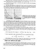
Evaluated sensitivity graphs of ω
0eq
- and Q
eq
-sensitivities on f

c
/ f
0
ratio in Fig. 10 and Fig. 11
show unsuitable values for higher x
c
. This fact limits the use of such biquads to lower values
of x
c
.
Fig. 10. S
ω
0eq
a
i
= f (x
c
)
Fig. 11. S
Q
eq
a
i
= f (x
c
)
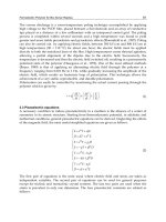
The modified structures containing integrators or differentiators show better sensitivity prop-
erties as is evident from Fig.12 and Fig. 13. The graphs pertain to the non-inverting BD inte-
grator version of Case I structure; similar behavior was found in versions based on FD inte-
grators, mixed BD-FD integrator combinations or differentiator based circuits.

This behavior can be easily explained, because the introduced integrator- and differentiator-
type structures are in fact the special cases of SFG or state-variable based biquad design.
Note that the ω
0eq
and Q
eq
sensitivities to the gain constants α
i
,
i=1,2
of integrator- and
differentiator-type building blocks are typically 0.5 - 1 and decrease to the limit value S
Q
eq
a
i
=
0.5 for x
c
 1. Similar values were obtained in the case of ω
0eq
sensitivities. Table 1 illus-
trates the sensitivity properties of the chosen Case I structure versions for starting parameters
f
0
= 2 kHz, f
c
= 48 kHz, Q = 1/
√
2.

Here symbol "M" denotes the "original" structure containing SI memory cells, "BD int" denotes
the version using BD integrators and similarly "FD int" denotes the version using FD integra-
tors. Case "FD+BD int" corresponds to the arrangement where FB1 block is implemented as
the FD integrator and FB2 block as the BD integrator. The order of FBs is important, a changed
arrangement results in increased sensitivities. The last row contains sensitivity values for a BD
differentiator based circuit.
Common features of analog sampled-data and digital lters design 73
Fig. 8. Case I. SI circuit
Fig. 9. Case II. SI circuit
To obtain a more complex overview about the circuits behavior, the following versions were
considered:
1. The SI-FBs are realized by memory cells in compliance with the digital prototype. These
are simple in the case of direct form 1, multiple-output under Fig.2 in the case of direct
form 2. The weighted outputs are set using changed W/L output transistor ratios.
2. Memory cells are replaced by non-inverting BD and FD integrators.
3. SI-FBs are realized by BD differentiators under Fig. 4, described by the transfer function
H
(z) = α (1 − z
−1
).
The following evaluative criteria were used for comparing all the considered structures:
• Sensitivity properties: With respect to the discrete-time character of SI circuits, the "equiv-
alent sensitivity" approach has been applied. A more detailed explanation of this ap-
proach has been published in Ref. Tichá (2006), and it is shortly indicated in Section 5.
• Losses influence: The important imperfections of SI circuits are caused by parasitic out-
put conductances of SI cells. In the following, these parasitics will be characterized by
output conductance g
o
or by ratio x
g

=
g
m
g
o
, where g
m
represents transistor transcon-
ductance.
• Transistor parameters spread: With respect to the technological limitations, the limits of
spread α
= W/L of transistors are crucial. In our considerations the maximum available
spread is expected to be in the interval α
max
/α
min
< 50. In general, the given limit
influences the maximum ratio of sampling frequency f
c
to ω
0eq
.
The necessary symbolic analysis were made using MAPLE libraries PraSCan and PraCAn,
developed by Biˇcák & Hospodka (2006), Biˇcák et al. (1999) for symbolic and numerical analysis
of sampled-data circuits.
4.1 Results obtained
Sensitivity evaluation:
At first, let us consider the "original SI networks" under Figs. 8 and 9. The transfer function
of both structures corresponds directly to the Eq. (15), and the sensitivity properties can be
expressed using procedure described in Sec. 5 in the form (25) and (26), as the functions of pa-

rameters a
1
, a
2
. More suitable for practical design are the sensitivity functions of "continuous-
time" H
(s) parameters ω
0
, Q and sampling period T. In this case the sensitivities can be
expressed by (29) and (30).
Evaluated sensitivity graphs of ω
0eq
- and Q
eq
-sensitivities on f
c
/ f
0
ratio in Fig. 10 and Fig. 11
show unsuitable values for higher x
c
. This fact limits the use of such biquads to lower values
of x
c
.
Fig. 10. S
ω
0eq
a
i

= f (x
c
)
Fig. 11. S
Q
eq
a
i
= f (x
c
)
The modified structures containing integrators or differentiators show better sensitivity prop-
erties as is evident from Fig.12 and Fig. 13. The graphs pertain to the non-inverting BD inte-
grator version of Case I structure; similar behavior was found in versions based on FD inte-
grators, mixed BD-FD integrator combinations or differentiator based circuits.
This behavior can be easily explained, because the introduced integrator- and differentiator-
type structures are in fact the special cases of SFG or state-variable based biquad design.
Note that the ω
0eq
and Q
eq
sensitivities to the gain constants α
i
,
i=1,2
of integrator- and
differentiator-type building blocks are typically 0.5 - 1 and decrease to the limit value S
Q
eq
a

i
=
0.5 for x
c
 1. Similar values were obtained in the case of ω
0eq
sensitivities. Table 1 illus-
trates the sensitivity properties of the chosen Case I structure versions for starting parameters
f
0
= 2 kHz, f
c
= 48 kHz, Q = 1/
√
2.
Here symbol "M" denotes the "original" structure containing SI memory cells, "BD int" denotes
the version using BD integrators and similarly "FD int" denotes the version using FD integra-
tors. Case "FD+BD int" corresponds to the arrangement where FB1 block is implemented as
the FD integrator and FB2 block as the BD integrator. The order of FBs is important, a changed
arrangement results in increased sensitivities. The last row contains sensitivity values for a BD
differentiator based circuit.
Digital Filters74
Fig. 12. S
ω
0eq
a
i
= f (x
c
)

Fig. 13. S
Q
eq
a
i
= f (x
c
)
Type S
ω
0eq
a
1
S
ω
0eq
a
2
S
Q
eq
a
1
S
Q
eq
a
2
S
Q

eq
α
1
S
Q
eq
α
2
M -14.6 5.97 -14.1 8.42 - -
BD int 0.109 0.491 -1.29 0.693 -0.601 0.693
FD int -0.075 0.491 -0.739 0.323 -0.416 0.323
FD+BD int -0.092 0.508 -0.907 0.491 -0.416 0.491
BD diff -0.075 -0.416 -0.739 0.416 -0.323 0.416
Table 1. Sensitivity properties
Losses influence:
As mentioned, the finite output conductances of the basic SI cells and current copiers (current
mirrors) are crucial in SI circuit design together with the number of blocks in the signal path.
With regard to this, it is necessary to distinguish between the Case I and Case II structures.
Some simulations showed slightly better behavior of the Case II arrangement. Simultane-
ously it is important to take into account the finite "on" resistance of switches. Especially
differentiator-based circuits are sensitive to switch imperfections.
Table 2 documents typical frequency response errors for the realizations introduced in Table1.
Here the typical ratios x
g
= g
m
/g
o
= 200 and r
on

switches equal to the input resistance of
current building blocks were considered.
Transistor parameters spread
This is markedly determined by the designed structure type and f
c
/ f
0
ratio. For illustration,
let us assume the LP biquad designed under the same conditions documented in Table 1 and
Table 2.
As is evident from Table 3, the maximum values spread shows the memory cell based version,
the max-to-min ratio equals 114.3. The differentiator and integrator based versions are less
demanding, the max-to-min ratio was evaluated from 48.5 to 69.9.
Type ε ε
max
ε(0) ε(ω
0
)
M-Case I 0.0346 0.426 0.426 0.176
M-Case II 0.0274 0.335 0.335 0.142
BD int Case I 0.0136 0.123 0.106 0.0853
BD int Case II 0.0147 0.139 0.126 0.0905
FD int Case I 0.0149 0.127 0.109 0.0915
BD diff Case I 0.0124 0.116 0.109 0.0458
Table 2. Frequency response errors
Note that the last versions have two free parameters α
1
, α
2
which can be exploited for design

optimization; unfortunately changes to these parameters do not allow any minimization of
values spread.
Type b
0
b
1
b
2
a
1
a
2
M 0.0143 0.285 0.0143 -1.635 0.692
BD int 0.0143
0.057
α
1
0.057
α
1
α
2
0.365
α
1
0.057
α
1
α
2

FD int 0.0206
0.0824
α
1
0.0824
α
1
α
2
−
0.3626
α
1
0.0824
α
1
α
2
FD+BD int 0.0206 0
0.0824
α
1
α
2
−
0.445
α
1
0.0824
α

1
α
2
BD diff 1 −
1
α
1
−
0.25
α
1
α
2
4.402
α
12.139
α
1
α
2
Table 3. design parameters for f
0
= 2 kHz
Type b
0
b
1
b
2
a

1
a
2
M 0.00391 0.00781 0.00391 -1.816 0.831
BD int 0.00391
0.0156
α
1
0.0156
α
1
α
2
0.184
α
1
0.0156
α
1
α
2
FD int 0.0047
0.0188
α
1
0.0188
α
1
α
2

−
0.184
α
1
0.0156
α
1
α
2
FD+BD int 0.0047 0
0.0188
α
1
α
2
−
0.203
α
1
0.0188
α
1
α
2
BD diff 1 −
1
α
1
−
0.25

α
1
α
2
9.804
α
53.21
α
1
α
2
Table 4. design parameters for f
0
= 1 kHz
The influence of the f
c
/ f
0
ratio to the transistor parameters spread is demonstrated in Table 4,
showing parameter changes for the lowered f
0
= 1 kHz from the previous design.
Common features of analog sampled-data and digital lters design 75
Fig. 12. S
ω
0eq
a
i
= f (x
c

)
Fig. 13. S
Q
eq
a
i
= f (x
c
)
Type S
ω
0eq
a
1
S
ω
0eq
a
2
S
Q
eq
a
1
S
Q
eq
a
2
S

Q
eq
α
1
S
Q
eq
α
2
M -14.6 5.97 -14.1 8.42 - -
BD int 0.109 0.491 -1.29 0.693 -0.601 0.693
FD int -0.075 0.491 -0.739 0.323 -0.416 0.323
FD+BD int -0.092 0.508 -0.907 0.491 -0.416 0.491
BD diff -0.075 -0.416 -0.739 0.416 -0.323 0.416
Table 1. Sensitivity properties
Losses influence:
As mentioned, the finite output conductances of the basic SI cells and current copiers (current
mirrors) are crucial in SI circuit design together with the number of blocks in the signal path.
With regard to this, it is necessary to distinguish between the Case I and Case II structures.
Some simulations showed slightly better behavior of the Case II arrangement. Simultane-
ously it is important to take into account the finite "on" resistance of switches. Especially
differentiator-based circuits are sensitive to switch imperfections.
Table 2 documents typical frequency response errors for the realizations introduced in Table1.
Here the typical ratios x
g
= g
m
/g
o
= 200 and r

on
switches equal to the input resistance of
current building blocks were considered.
Transistor parameters spread
This is markedly determined by the designed structure type and f
c
/ f
0
ratio. For illustration,
let us assume the LP biquad designed under the same conditions documented in Table 1 and
Table 2.
As is evident from Table 3, the maximum values spread shows the memory cell based version,
the max-to-min ratio equals 114.3. The differentiator and integrator based versions are less
demanding, the max-to-min ratio was evaluated from 48.5 to 69.9.
Type ε ε
max
ε(0) ε(ω
0
)
M-Case I 0.0346 0.426 0.426 0.176
M-Case II 0.0274 0.335 0.335 0.142
BD int Case I 0.0136 0.123 0.106 0.0853
BD int Case II 0.0147 0.139 0.126 0.0905
FD int Case I 0.0149 0.127 0.109 0.0915
BD diff Case I 0.0124 0.116 0.109 0.0458
Table 2. Frequency response errors
Note that the last versions have two free parameters α
1
, α
2

which can be exploited for design
optimization; unfortunately changes to these parameters do not allow any minimization of
values spread.
Type b
0
b
1
b
2
a
1
a
2
M 0.0143 0.285 0.0143 -1.635 0.692
BD int 0.0143
0.057
α
1
0.057
α
1
α
2
0.365
α
1
0.057
α
1
α

2
FD int 0.0206
0.0824
α
1
0.0824
α
1
α
2
−
0.3626
α
1
0.0824
α
1
α
2
FD+BD int 0.0206 0
0.0824
α
1
α
2
−
0.445
α
1
0.0824

α
1
α
2
BD diff 1 −
1
α
1
−
0.25
α
1
α
2
4.402
α
12.139
α
1
α
2
Table 3. design parameters for f
0
= 2 kHz
Type b
0
b
1
b
2

a
1
a
2
M 0.00391 0.00781 0.00391 -1.816 0.831
BD int 0.00391
0.0156
α
1
0.0156
α
1
α
2
0.184
α
1
0.0156
α
1
α
2
FD int 0.0047
0.0188
α
1
0.0188
α
1
α

2
−
0.184
α
1
0.0156
α
1
α
2
FD+BD int 0.0047 0
0.0188
α
1
α
2
−
0.203
α
1
0.0188
α
1
α
2
BD diff 1 −
1
α
1
−

0.25
α
1
α
2
9.804
α
53.21
α
1
α
2
Table 4. design parameters for f
0
= 1 kHz
The influence of the f
c
/ f
0
ratio to the transistor parameters spread is demonstrated in Table 4,
showing parameter changes for the lowered f
0
= 1 kHz from the previous design.
Digital Filters76
In this case the max-to-min ratio increases for the memory cell version to 464.4. The best result
is obtained for the differentiator based circuit, where the max-to-min ratio equals 212.8. It is
evident that such designs are hardly realizable and strongly require lower sampling frequency.
5. Sensitivity approach in discrete-time filters design
The sensitivity approach is a worthwile tool for the optimized design of analog continuous-
time and sampled-data filters. Particularly the design of biquadratic sections for cascade re-

alization of higher-order filters is significantly influenced by the sensitivity properties of the
considered circuits. Mainly the sensitivities of ω
0
- and Q- parameters to the filter elements
changes serve as the effective criterion for suitable circuit structure selection and design opti-
mization, because ω
0
and Q uniquely determine the frequency response shape.
The ”main“ sensitivities of the biquadratic transfer function H
(s) (16) are defined by formulas
(17), where x
i
means active and passive circuit elements. The ω
0
and Q parameters are defined
by (18) as the functions of the real and imaginary parts σ
1
, ω
1
of the complex-conjugate poles
of the 2
nd
-order biquadratic transfer function (16).
H
(s) =
k
2
s
2
+ k

1
s + k
0
s
2
+
ω
0
Q
s + ω
2
0
(16)
S
ω
0
x
i
=
∂ω
0
∂x
i
x
i
ω
0
; S
Q
x

i
=
∂Q
∂x
i
x
i
Q
; (17)
ω
0
=

σ
2
1
+ ω
2
1
; Q =
ω
0
2 σ
1
. (18)
Sensitivity concept is less usual in the field of the digital filters, because there is not a direct
equivalent of the ω
0
and Q parameters in the s-plane to the similar parameters in z-plane.
Nevertheless the relevance of sensitivity usage in digital filter design can be more obvious, if

we are aware of the correspondence between rounding errors in "digital area" and tolerances
of circuit element values in the "continuous-time" area. Here the sensitivities represent the
measure for possible rounding without loss of the accuracy of the filter frequency response.
Simultaneously, sensitivities can help to solve problems with the optimum choice of the real-
ization structure with respect to the ”non-standard” design conditions, e.g. in design of the
digital filters and equalizers for audio signal processing.
To apply sensitivity approach in digital filter design effectively, it is necessary to formularize
equivalent sensitivity parameters, transforming z-plane parameters into s-plane and evaluate
them like functions of H
(z). Such a procedure, described in Tichá (2006), will be presented in
the following.
5.1 Equivalent sensitivity evaluation
Let us assume "standard" 2
nd
-order transfer function H (z) in the form (19). The equivalent
parameters ω
0
and Q can be obtained using an appropriate transformation of H(z) into s-
plane and comparison to the ordinary form of H
(s) under (16)
H
(z) =
b
0
+ b
1
z
−1
+ b
2

z
−2
1 − a
1
z
−1
− a
2
z
−2
; (19)
To obtain the generally valid relationship, the z
−s transformation should be symbolic. Using
inverse bilinear transformation (20) of H
(z)
z =
2 + s T
2
−s T
(20)
we obtain equivalent H
eq
(s) in the form (21) and after formal rearrangement the final form
(22) comparable to (16).
H
eq
(s) =
T
2
(

b
0
−b
1
+ b
2
)
s
2
+ 4 T
(
b
0
−b
2
)
s + 4
(
b
0
+ b
1
+ b
2
)
T
2
(
1 + a
1

−a
2
)
s
2
+ 4 T
(
a
2
+ 1
)
s + 4
(
1 − a
1
−a
2
)
; (21)
H
eq
(s) =
(
b
0
−b
1
+b
2
)

1+a
1
−a
2
s
2
+ 4
(
b
0
−b
2
)
T
(
1+a
1
−a
2
)
s + 4
b
0
+b
1
+b
2
T
2
(

1+a
1
−a
2
)
s
2
+ 4
(
a
2
+1
)
T
(
1+a
1
−a
2
)
s + 4
1−a
1
−a
2
T
2
(
1+a
1

−a
2
)
. (22)
A comparison of (22) to (16) gives
ω
0eq
=
2
T

1
− a
1
− a
2
1 + a
1
− a
2
; (23)
Q
eq
=

(1 −a
2
)
2
− a

2
1
2 (1 + a
2
)
. (24)
Now it is possible to express the equivalent sensitivity of ω
0eq
and Q
eq
to the denominator
coefficients a
1
and a
2
using formula (17). The symbolic form of the evaluated sensitivities is
as follows
S
ω
0
a
1
= −
a
1
(1 −a
2
)
(
1 − a

2
)
2
−a
2
1
; S
Q
a
1
= −
a
1
2
(1 −a
2
)
2
−a
2
1
; (25)
S
ω
0
a
2
=
a
1

a
2
(1 −a
2
)
2
−a
2
1
; S
Q
a
2
=
a
2

a
1
2
−2 (1 −a
2
)

(1 + a
2
)

(1 −a
2

)
2
−a
2
1

. (26)
In some cases it is suitable to express the equivalent sensitivities as the functions of ω
0
, Q and
T, or x
c
= f
c
/ω
0
. To extend the expressions (25) - (26), it is necessary to transform coefficients
a
1
, a
2
into s-plane using backward bilinear transformation of H(z) denominator. Doing this,
the following expressions were gained:
a
1
=
2 (4 − ω
2
0
T

2
) Q
2 ω
0
T + 4 Q + ω
2
0
T
2
Q
; (27)
a
2
= −
−
2 ω
0
T + ω
2
0
T
2
Q + 4Q
2 ω
0
T + 4 Q + ω
2
0
T
2

Q
. (28)
Applying (27) and (28) in Eqs. (25) to (26) we obtain the modified sensitivity expressions (29)
– (30). The parameter x
c
is defined by Eq. (31).
S
ω
0
a
1
e
= −
(
16 x
4
c
−1)
16 x
2
c
; S
Q
a
1
e
= −
(
4 x
2

c
−1)
2
16 x
2
c
; (29)
S
ω
0
a
2
e
=
x
2
c
2
−
x
c
4 Q
+
1
16 x
c
Q
−
1
32 x

2
c
; S
Q
a
2
e
= −
1
4
+
x
2
c
2
+
(
1 + 4x
c
) (4Q
2
−1)
16 Q x
c
+
1
32 x
2
c
. (30)

x
c
=
1
T ω
0
=
f
c
ω
0
(31)
Common features of analog sampled-data and digital lters design 77
In this case the max-to-min ratio increases for the memory cell version to 464.4. The best result
is obtained for the differentiator based circuit, where the max-to-min ratio equals 212.8. It is
evident that such designs are hardly realizable and strongly require lower sampling frequency.
5. Sensitivity approach in discrete-time filters design
The sensitivity approach is a worthwile tool for the optimized design of analog continuous-
time and sampled-data filters. Particularly the design of biquadratic sections for cascade re-
alization of higher-order filters is significantly influenced by the sensitivity properties of the
considered circuits. Mainly the sensitivities of ω
0
- and Q- parameters to the filter elements
changes serve as the effective criterion for suitable circuit structure selection and design opti-
mization, because ω
0
and Q uniquely determine the frequency response shape.
The ”main“ sensitivities of the biquadratic transfer function H
(s) (16) are defined by formulas
(17), where x

i
means active and passive circuit elements. The ω
0
and Q parameters are defined
by (18) as the functions of the real and imaginary parts σ
1
, ω
1
of the complex-conjugate poles
of the 2
nd
-order biquadratic transfer function (16).
H
(s) =
k
2
s
2
+ k
1
s + k
0
s
2
+
ω
0
Q
s + ω
2

0
(16)
S
ω
0
x
i
=
∂ω
0
∂x
i
x
i
ω
0
; S
Q
x
i
=
∂Q
∂x
i
x
i
Q
; (17)
ω
0

=

σ
2
1
+ ω
2
1
; Q =
ω
0
2 σ
1
. (18)
Sensitivity concept is less usual in the field of the digital filters, because there is not a direct
equivalent of the ω
0
and Q parameters in the s-plane to the similar parameters in z-plane.
Nevertheless the relevance of sensitivity usage in digital filter design can be more obvious, if
we are aware of the correspondence between rounding errors in "digital area" and tolerances
of circuit element values in the "continuous-time" area. Here the sensitivities represent the
measure for possible rounding without loss of the accuracy of the filter frequency response.
Simultaneously, sensitivities can help to solve problems with the optimum choice of the real-
ization structure with respect to the ”non-standard” design conditions, e.g. in design of the
digital filters and equalizers for audio signal processing.
To apply sensitivity approach in digital filter design effectively, it is necessary to formularize
equivalent sensitivity parameters, transforming z-plane parameters into s-plane and evaluate
them like functions of H
(z). Such a procedure, described in Tichá (2006), will be presented in
the following.

5.1 Equivalent sensitivity evaluation
Let us assume "standard" 2
nd
-order transfer function H (z) in the form (19). The equivalent
parameters ω
0
and Q can be obtained using an appropriate transformation of H(z) into s-
plane and comparison to the ordinary form of H
(s) under (16)
H
(z) =
b
0
+ b
1
z
−1
+ b
2
z
−2
1 − a
1
z
−1
− a
2
z
−2
; (19)

To obtain the generally valid relationship, the z
−s transformation should be symbolic. Using
inverse bilinear transformation (20) of H
(z)
z =
2 + s T
2 − s T
(20)
we obtain equivalent H
eq
(s) in the form (21) and after formal rearrangement the final form
(22) comparable to (16).
H
eq
(s) =
T
2
(
b
0
−b
1
+ b
2
)
s
2
+ 4 T
(
b

0
−b
2
)
s + 4
(
b
0
+ b
1
+ b
2
)
T
2
(
1 + a
1
−a
2
)
s
2
+ 4 T
(
a
2
+ 1
)
s + 4

(
1 − a
1
−a
2
)
; (21)
H
eq
(s) =
(
b
0
−b
1
+b
2
)
1+a
1
−a
2
s
2
+ 4
(
b
0
−b
2

)
T
(
1+a
1
−a
2
)
s + 4
b
0
+b
1
+b
2
T
2
(
1+a
1
−a
2
)
s
2
+ 4
(
a
2
+1

)
T
(
1+a
1
−a
2
)
s + 4
1−a
1
−a
2
T
2
(
1+a
1
−a
2
)
. (22)
A comparison of (22) to (16) gives
ω
0eq
=
2
T

1 − a

1
− a
2
1 + a
1
− a
2
; (23)
Q
eq
=

(1 −a
2
)
2
− a
2
1
2 (1 + a
2
)
. (24)
Now it is possible to express the equivalent sensitivity of ω
0eq
and Q
eq
to the denominator
coefficients a
1

and a
2
using formula (17). The symbolic form of the evaluated sensitivities is
as follows
S
ω
0
a
1
= −
a
1
(1 −a
2
)
(1 −a
2
)
2
−a
2
1
; S
Q
a
1
= −
a
1
2

(1 −a
2
)
2
−a
2
1
; (25)
S
ω
0
a
2
=
a
1
a
2
(1 −a
2
)
2
−a
2
1
; S
Q
a
2
=

a
2

a
1
2
−2 (1 −a
2
)

(1 + a
2
)

(1 −a
2
)
2
−a
2
1

. (26)
In some cases it is suitable to express the equivalent sensitivities as the functions of ω
0
, Q and
T, or x
c
= f
c

/ω
0
. To extend the expressions (25) - (26), it is necessary to transform coefficients
a
1
, a
2
into s-plane using backward bilinear transformation of H(z) denominator. Doing this,
the following expressions were gained:
a
1
=
2 (4 − ω
2
0
T
2
) Q
2 ω
0
T + 4 Q + ω
2
0
T
2
Q
; (27)
a
2
= −

−
2 ω
0
T + ω
2
0
T
2
Q + 4Q
2 ω
0
T + 4 Q + ω
2
0
T
2
Q
. (28)
Applying (27) and (28) in Eqs. (25) to (26) we obtain the modified sensitivity expressions (29)
– (30). The parameter x
c
is defined by Eq. (31).
S
ω
0
a
1
e
= −
(

16 x
4
c
−1)
16 x
2
c
; S
Q
a
1
e
= −
(
4 x
2
c
−1)
2
16 x
2
c
; (29)
S
ω
0
a
2
e
=

x
2
c
2
−
x
c
4 Q
+
1
16 x
c
Q
−
1
32 x
2
c
; S
Q
a
2
e
= −
1
4
+
x
2
c

2
+
(
1 + 4x
c
) (4Q
2
−1)
16 Q x
c
+
1
32 x
2
c
. (30)
x
c
=
1
T ω
0
=
f
c
ω
0
(31)
Digital Filters78
The formulas obtained are valid directly for the 1

st
and the 2
nd
canonic direct form of the
digital filters – see Laipert et al. (2000), Antoniou (1979), Mitra (2005) and others. For the
other 2
nd
-order structures it is necessary to express the transfer function H(z) coefficients
a
i
, b
i
,
i=0,1,2
(19) as the functions of the analyzed structure parameters. The practical use of
this will be explained in the following parts.
5.2 Sensitivity properties of the direct canonic forms of digital filters
As mentioned, the sensitivity properties to the parameters of the 1
st
and the 2
nd
direct form
of the digital 2
nd
-order filters are straightly specified by above presented formulas, because
the coefficients are determined by the multipliers and adders constants of the filter block di-
agram. The filter general sensitivity properties can be in this case characterized preferably
by modified equations (29) and (30) as the functions of equivalent Q-factor and the ratio x
c
given by eq. (31). The following figures Fig. 14 and Fig. 15 show the sensitivity S

ω
0eq
a
1,2
and S
Q
eq
a
1,2
as functions of Q
eq
.
Fig. 14. S
ω
0
a
1,2
= f (Q)
Fig. 15. S
Q
a
1,2
= f (Q)
As evident, S
ω
0eq
a
1
together with S
Q

eq
a
1
do not depend on Q-factor value, in contrast to the S
ω
0
a
2
sensitivities. Note that sensitivities values are higher in comparison to the similar analogue
realizations.
From the practical point-of-view the Figs. 16 and 17 are more important. Here the S
ω
0eq
a
1,2
and
S
Q
eq
a
1,2
sensitivities are depicted in dependence of ratio x
c
, thus indirectly as the functions of ω
0eq
and T. These sensitivities are significantly higher than the previous ones and rapidly increase
for x
c
≥ 10. This bears to the known fact, that direct forms of digital filters are less appropriate
for such implementations, where the sampling frequency is relative high.

5.3 Digital filters derived from SFG graph
These filters are analogous to the continuous-time 2
nd
-order filters designed on two-integrator
feedback loop. A typical example of such a filter is shown in Fig.18. Transfer function of
this filter given by Eq. (32) was evaluated using modified SYRUP library in the mathematical
program MAPLE – see Tichá & Martinek (2007).
Fig. 16. S
ω
0
a
1,2
= f (x)
Fig. 17. S
Q
a
1,2
= f (x)
A sensitivity evaluation was made according to the previous example. The results are as
follows:
H
(z) =
a
5
z
2
+ (a
1
−a
5

+ a
6
) z −a
6
(1 −a
4
) z
2
−(2 + a
2
−a
4
) z + 1
; (32)
ω
0eq
=
2
T

−
a
2
4 + a
2
−2 a
4
; (33)
Q
eq

=

a
2
(
2 a
4
− a
2
−4
)
2 a
4
. (34)
The corresponding sensitivities of ω
0eq
and Q
eq
to the H(z) denominator coefficients a
i
have
the form (35) to (38), and the modified sensitivities the form (39) to (42). Note that parameter
x
c
is defined by Eq. (31)
S
ω
0
a
2

=
2 − a
4
4 + a
2
−2 a
4
; (35) S
Q
a
2
=
2 + a
2
−a
4
4 + a
2
−2 a
4
; (36)
S
ω
0
a
4
=
a
4
4 + a

2
−2 a
4
; (37)
S
Q
a
4
= −
4 + a
2
−a
4
4 + a
2
−2 a
4
; (38)
S
ω
0
a
2
m
=
1
2
+
1
8 x

2
c
; (39) S
Q
a
2
m
=
1
2
−
1
8 x
2
c
; (40)
S
ω
0
a
4
m
= −
1
4 x
c
Q
; (41) S
Q
a

4
m
= −1 +
1
4 x
c
Q
. (42)
Similarly to the previous example the evaluated sensitivities can be presented as the functions
of Q and x
c
. The graphical representation of the functions S
ω
0
a
i
= f (Q) and S
Q
a
i
= f (Q);
i=2,3,4
for given x
c
= 5 is in Fig. 19. The graphs of functions S
ω
0
a
i
= f (x

c
) and S
Q
a
i
= f (x
c
);
i=2,4
for
Q
= 2 are shown in Figs. 20.
Common features of analog sampled-data and digital lters design 79
The formulas obtained are valid directly for the 1
st
and the 2
nd
canonic direct form of the
digital filters – see Laipert et al. (2000), Antoniou (1979), Mitra (2005) and others. For the
other 2
nd
-order structures it is necessary to express the transfer function H(z) coefficients
a
i
, b
i
,
i=0,1,2
(19) as the functions of the analyzed structure parameters. The practical use of
this will be explained in the following parts.

5.2 Sensitivity properties of the direct canonic forms of digital filters
As mentioned, the sensitivity properties to the parameters of the 1
st
and the 2
nd
direct form
of the digital 2
nd
-order filters are straightly specified by above presented formulas, because
the coefficients are determined by the multipliers and adders constants of the filter block di-
agram. The filter general sensitivity properties can be in this case characterized preferably
by modified equations (29) and (30) as the functions of equivalent Q-factor and the ratio x
c
given by eq. (31). The following figures Fig. 14 and Fig. 15 show the sensitivity S
ω
0eq
a
1,2
and S
Q
eq
a
1,2
as functions of Q
eq
.
Fig. 14. S
ω
0
a

1,2
= f (Q)
Fig. 15. S
Q
a
1,2
= f (Q)
As evident, S
ω
0eq
a
1
together with S
Q
eq
a
1
do not depend on Q-factor value, in contrast to the S
ω
0
a
2
sensitivities. Note that sensitivities values are higher in comparison to the similar analogue
realizations.
From the practical point-of-view the Figs. 16 and 17 are more important. Here the S
ω
0eq
a
1,2
and

S
Q
eq
a
1,2
sensitivities are depicted in dependence of ratio x
c
, thus indirectly as the functions of ω
0eq
and T. These sensitivities are significantly higher than the previous ones and rapidly increase
for x
c
≥ 10. This bears to the known fact, that direct forms of digital filters are less appropriate
for such implementations, where the sampling frequency is relative high.
5.3 Digital filters derived from SFG graph
These filters are analogous to the continuous-time 2
nd
-order filters designed on two-integrator
feedback loop. A typical example of such a filter is shown in Fig.18. Transfer function of
this filter given by Eq. (32) was evaluated using modified SYRUP library in the mathematical
program MAPLE – see Tichá & Martinek (2007).
Fig. 16. S
ω
0
a
1,2
= f (x)
Fig. 17. S
Q
a

1,2
= f (x)
A sensitivity evaluation was made according to the previous example. The results are as
follows:
H
(z) =
a
5
z
2
+ (a
1
−a
5
+ a
6
) z −a
6
(1 −a
4
) z
2
−(2 + a
2
−a
4
) z + 1
; (32)
ω
0eq

=
2
T

−
a
2
4 + a
2
−2 a
4
; (33)
Q
eq
=

a
2
(
2 a
4
− a
2
−4
)
2 a
4
. (34)
The corresponding sensitivities of ω
0eq

and Q
eq
to the H(z) denominator coefficients a
i
have
the form (35) to (38), and the modified sensitivities the form (39) to (42). Note that parameter
x
c
is defined by Eq. (31)
S
ω
0
a
2
=
2 − a
4
4 + a
2
−2 a
4
; (35) S
Q
a
2
=
2 + a
2
−a
4

4 + a
2
−2 a
4
; (36)
S
ω
0
a
4
=
a
4
4 + a
2
−2 a
4
; (37)
S
Q
a
4
= −
4 + a
2
−a
4
4 + a
2
−2 a

4
; (38)
S
ω
0
a
2
m
=
1
2
+
1
8 x
2
c
; (39) S
Q
a
2
m
=
1
2
−
1
8 x
2
c
; (40)

S
ω
0
a
4
m
= −
1
4 x
c
Q
; (41) S
Q
a
4
m
= −1 +
1
4 x
c
Q
. (42)
Similarly to the previous example the evaluated sensitivities can be presented as the functions
of Q and x
c
. The graphical representation of the functions S
ω
0
a
i

= f (Q) and S
Q
a
i
= f (Q);
i=2,3,4
for given x
c
= 5 is in Fig. 19. The graphs of functions S
ω
0
a
i
= f (x
c
) and S
Q
a
i
= f (x
c
);
i=2,4
for
Q
= 2 are shown in Figs. 20.
Digital Filters80
Fig. 18. Digital 2
nd
-order integrator-based filter

(a) S
ω
0
a
2,4
= f (Q) (b) S
Q
a
2,4
= f (Q)
Fig. 19. Sensitivities S
ω
0
a
2,4
= f (Q) and S
Q
a
2,4
= f (Q) for x
c
= 5.
In comparison to the direct-form structure all the sensitivities are considerably smaller and do
not exceed unit value. It is important to emphasize the sensitivity independence from ratio x
c
.
It means that such a filter can be implemented successfully under non-standard conditions,
where the limited word length or high ratio of ω
0
and f

c
lead to the significant frequency
response inaccuracy or filter instability.
(a) S
ω
0
a
2,4
= f (x) (b) S
Q
a
2,4
= f (x)
Fig. 20. Sensitivities S
ω
0
a
2,4
= f(x
c
) and S
Q
a
2,4
= f(x
c
) for Q = 2.
6. A tool for symbolic analysis of digital filters
Symbolic and semi-symbolic analysis is considered to be an efficient tool for design and op-
timization of electrical and electronic circuits, not only analogue, but also digital. During

the last period many specialized programs were developed for this purpose, but the most of
them do not allow the direct post-processing of the results obtained. The more prospective
approach is based on the use of mathematical programs oriented to the symbolic mathemat-
ics. Here the MAPLE program, especially developed for symbolic computations, seems to be
the most suitable for this purpose. The symbolic analysis of analogue circuit is supported in
MAPLE program by the SYRUP library Riel (2007). The SYRUP represents simple, but very ef-
ficient universal tool for circuit analysis, similar to the SPICE program in the circuit numerical
analysis area.
As shown in the following, the SYRUP library can be easily adapted for the digital filters sym-
bolic analysis as well. This assertion results from the fact, that circuit equations describing the
digital filter block diagrams are very similar to the ones describing common analogue circuits.
It leads to the direct use of the modified node-voltage equations method after completing the
basic elements library. In contrast to the commonly used programs for circuit analysis, the
input language of the SYRUP library is very flexible and allows to create models of the digital
filter building block by a simple way.
6.1 The MAPLE-SYRUP library extension
To analyze digital filter block diagrams using SYRUP, it is necessary to complete the basic set
of circuit elements models. The most important "digital" building blocks are the delay element
D and general multiple-input summing element SUM. The first of them is presented in Fig. 21
and the second in Fig. 22. Note that A in the summing element equation means summer
gain; i.e. the multiplication operation can be included into this element. Nevertheless, the
multiplication can be realized independently as well by some of "standard" library elements.
Common features of analog sampled-data and digital lters design 81
Fig. 18. Digital 2
nd
-order integrator-based filter
(a) S
ω
0
a

2,4
= f (Q) (b) S
Q
a
2,4
= f (Q)
Fig. 19. Sensitivities S
ω
0
a
2,4
= f (Q) and S
Q
a
2,4
= f (Q) for x
c
= 5.
In comparison to the direct-form structure all the sensitivities are considerably smaller and do
not exceed unit value. It is important to emphasize the sensitivity independence from ratio x
c
.
It means that such a filter can be implemented successfully under non-standard conditions,
where the limited word length or high ratio of ω
0
and f
c
lead to the significant frequency
response inaccuracy or filter instability.
(a) S

ω
0
a
2,4
= f (x) (b) S
Q
a
2,4
= f (x)
Fig. 20. Sensitivities S
ω
0
a
2,4
= f(x
c
) and S
Q
a
2,4
= f(x
c
) for Q = 2.
6. A tool for symbolic analysis of digital filters
Symbolic and semi-symbolic analysis is considered to be an efficient tool for design and op-
timization of electrical and electronic circuits, not only analogue, but also digital. During
the last period many specialized programs were developed for this purpose, but the most of
them do not allow the direct post-processing of the results obtained. The more prospective
approach is based on the use of mathematical programs oriented to the symbolic mathemat-
ics. Here the MAPLE program, especially developed for symbolic computations, seems to be

the most suitable for this purpose. The symbolic analysis of analogue circuit is supported in
MAPLE program by the SYRUP library Riel (2007). The SYRUP represents simple, but very ef-
ficient universal tool for circuit analysis, similar to the SPICE program in the circuit numerical
analysis area.
As shown in the following, the SYRUP library can be easily adapted for the digital filters sym-
bolic analysis as well. This assertion results from the fact, that circuit equations describing the
digital filter block diagrams are very similar to the ones describing common analogue circuits.
It leads to the direct use of the modified node-voltage equations method after completing the
basic elements library. In contrast to the commonly used programs for circuit analysis, the
input language of the SYRUP library is very flexible and allows to create models of the digital
filter building block by a simple way.
6.1 The MAPLE-SYRUP library extension
To analyze digital filter block diagrams using SYRUP, it is necessary to complete the basic set
of circuit elements models. The most important "digital" building blocks are the delay element
D and general multiple-input summing element SUM. The first of them is presented in Fig. 21
and the second in Fig. 22. Note that A in the summing element equation means summer
gain; i.e. the multiplication operation can be included into this element. Nevertheless, the
multiplication can be realized independently as well by some of "standard" library elements.
Digital Filters82
Y
out
(z) =
[
X
a
(z) + X
b
(z)
]
z

−1
>
.subckt MEM out a b
>
Vout out 0
(v[a]+v[b])/z
>
.ends
Fig. 21. The Delay element model
Y
out
(z) = A
[
X
a
(z) + X
b
(z) + X
c
(z)
]
>
.subckt SUM out a b c
>
Vout out 0
A
*
(v[a]+v[b]+v[c])
>
.ends

Fig. 22. The general summer model
All the mentioned blocks can be represented by sub-circuits, based on "voltage" description,
as demonstrated by listings in SYRUP language – see Fig. 21 and 22. It is important to say
that the multiple-input delay element model can be easily created, and, in this modified form
it makes possible significant simplification of the block diagram and its description in the
SYRUP input file.
6.2 Post-processing of the results
The MAPLE program environment offers an efficient processing of the symbolic terms includ-
ing simplification of algebraic expressions, solution of the sets of symbolic or semi-symbolic
equations, symbolic differentiation or integration and so forth. This gives facilities for effec-
tive post-processing of the symbolic analysis results, especially for the purpose of the analyzed
networks optimized design. The following topics can be typically solved:
• Derivation of the design formulas.
The "standard" procedure compares the given numerical transfer function with the sym-
bolic one of the filter designed. It leads to the system of equations for unknown parame-
ters of building blocks (usually multipliers). In the case of the direct form structures the
design procedure is the simplest with respect to the canonical character of the solved
filter. The general solution of design formulas for the uncanonical structures is not so
simple and usually requires any auxiliary tool.
Design of the IIR filters usually starts from the prewarped continuous-time transfer
function H
(s), obtained using approximation procedure. Here the necessary H(s) →
H(z) transformation can be integrated with the designed filter parameters computa-
tion, similarly to the design of analogue sampled-data filters. Especially for the 2
nd
-
order partial transfer functions it is easy to derive the direct formulas based on H
(s)
parameters ω
0

and Q. The use for cascade realization of the higher-order digital filters
is evident.
• Sensitivity properties computations.
The relevance of sensitivity computation in digital filter design can be more obvious,
if we are aware of the correspondence between rounding errors in "digital area" and
tolerances of element values in the "continuous-time area". Therein the sensitivities
represent the measure for possible rounding without loss of the accuracy of the filter
frequency response.
• Optimization with respect to the building blocks parameter values spread, dynamics and sensi-
tivity properties.
The dynamics optimization is important with respect to the data-overflow. The op-
timization is based on the partial transfer maxims comparison and their equalization
with respect to the "main" transfer maximum. The optimization procedure can be sup-
ported by symbolic partial transfers computation and the critical parameter finding. As
proved, symbolic analysis is the excellent tool for complex optimization solving all the
mentioned criteria.
6.3 Examples
The usage of the extended library is demonstrated on the analysis of some typical examples of
digital filters, represented by block diagrams. Note that the obtained transfer functions H
(z)
can be easily post-processed in MAPLE environment and used for the optimized design of the
simulated systems.
The simplest example of symbolic analysis seems to be the 2
nd
-order digital filter direct form
II. structure. The block diagram is shown in Fig.23 and the SYRUP data file in the Fig. 24.
HK2 :
=
b0 z
2

+ b1 z + b2
z
2
+ a1 z + a2
Fig. 23. The 2
nd
-order direct form II.
>
obvod5:= "
>
Vn 1 0
>
XS1 3 1 7 0 SUM(A=1)
>
XS2 7 6 11 0 SUM(A=1)
>
XM1 5 3 0 MEM
>
XM2 10 5 0 MEM
>
Ea1 6 0 5 0 -a1
>
Ea2 11 0 10 0 -a2
>
Eb0 4 0 3 0 b0
>
Eb1 8 0 5 0 b1
>
XS3 9 12 8 0 SUM(A=1)
>

Eb2 12 0 10 0 b2
>
XS4 2 4 9 0 SUM(A=1)
>
.subckt SUM out a b c
>
Vd out 0
A
*
(v[a]+v[b]+v[c])
>
.ends
>
.subckt MEM out a b
>
Vg out 0 (v[a]+v[b])/z
>
.ends
>
.end ":
Fig. 24. Data-file SYRUP
Common features of analog sampled-data and digital lters design 83
Y
out
(z) =
[
X
a
(z) + X
b

(z)
]
z
−1
>
.subckt MEM out a b
>
Vout out 0
(v[a]+v[b])/z
>
.ends
Fig. 21. The Delay element model
Y
out
(z) = A
[
X
a
(z) + X
b
(z) + X
c
(z)
]
>
.subckt SUM out a b c
>
Vout out 0
A
*

(v[a]+v[b]+v[c])
>
.ends
Fig. 22. The general summer model
All the mentioned blocks can be represented by sub-circuits, based on "voltage" description,
as demonstrated by listings in SYRUP language – see Fig. 21 and 22. It is important to say
that the multiple-input delay element model can be easily created, and, in this modified form
it makes possible significant simplification of the block diagram and its description in the
SYRUP input file.
6.2 Post-processing of the results
The MAPLE program environment offers an efficient processing of the symbolic terms includ-
ing simplification of algebraic expressions, solution of the sets of symbolic or semi-symbolic
equations, symbolic differentiation or integration and so forth. This gives facilities for effec-
tive post-processing of the symbolic analysis results, especially for the purpose of the analyzed
networks optimized design. The following topics can be typically solved:
• Derivation of the design formulas.
The "standard" procedure compares the given numerical transfer function with the sym-
bolic one of the filter designed. It leads to the system of equations for unknown parame-
ters of building blocks (usually multipliers). In the case of the direct form structures the
design procedure is the simplest with respect to the canonical character of the solved
filter. The general solution of design formulas for the uncanonical structures is not so
simple and usually requires any auxiliary tool.
Design of the IIR filters usually starts from the prewarped continuous-time transfer
function H
(s), obtained using approximation procedure. Here the necessary H(s) →
H(z) transformation can be integrated with the designed filter parameters computa-
tion, similarly to the design of analogue sampled-data filters. Especially for the 2
nd
-
order partial transfer functions it is easy to derive the direct formulas based on H

(s)
parameters ω
0
and Q. The use for cascade realization of the higher-order digital filters
is evident.
• Sensitivity properties computations.
The relevance of sensitivity computation in digital filter design can be more obvious,
if we are aware of the correspondence between rounding errors in "digital area" and
tolerances of element values in the "continuous-time area". Therein the sensitivities
represent the measure for possible rounding without loss of the accuracy of the filter
frequency response.
• Optimization with respect to the building blocks parameter values spread, dynamics and sensi-
tivity properties.
The dynamics optimization is important with respect to the data-overflow. The op-
timization is based on the partial transfer maxims comparison and their equalization
with respect to the "main" transfer maximum. The optimization procedure can be sup-
ported by symbolic partial transfers computation and the critical parameter finding. As
proved, symbolic analysis is the excellent tool for complex optimization solving all the
mentioned criteria.
6.3 Examples
The usage of the extended library is demonstrated on the analysis of some typical examples of
digital filters, represented by block diagrams. Note that the obtained transfer functions H
(z)
can be easily post-processed in MAPLE environment and used for the optimized design of the
simulated systems.
The simplest example of symbolic analysis seems to be the 2
nd
-order digital filter direct form
II. structure. The block diagram is shown in Fig.23 and the SYRUP data file in the Fig. 24.
HK2 :=

b0 z
2
+ b1 z + b2
z
2
+ a1 z + a2
Fig. 23. The 2
nd
-order direct form II.
>
obvod5:= "
>
Vn 1 0
>
XS1 3 1 7 0 SUM(A=1)
>
XS2 7 6 11 0 SUM(A=1)
>
XM1 5 3 0 MEM
>
XM2 10 5 0 MEM
>
Ea1 6 0 5 0 -a1
>
Ea2 11 0 10 0 -a2
>
Eb0 4 0 3 0 b0
>
Eb1 8 0 5 0 b1
>

XS3 9 12 8 0 SUM(A=1)
>
Eb2 12 0 10 0 b2
>
XS4 2 4 9 0 SUM(A=1)
>
.subckt SUM out a b c
>
Vd out 0
A
*
(v[a]+v[b]+v[c])
>
.ends
>
.subckt MEM out a b
>
Vg out 0 (v[a]+v[b])/z
>
.ends
>
.end ":
Fig. 24. Data-file SYRUP
Digital Filters84
The presented structure does not require any special procedure for design formulas. On the
other hand, it could be interesting to analyze the sensitivity properties.
The obtained expressions are suitable for the estimation of the "starting continuous-time pa-
rameters" influence to the digital filter parameters changes. As an example, the following
graph in Fig.25 illustrates the S
Q

a
1
,a
2
sensitivity dependence on the Q-factor, when the ratio
x
c
=
f
c
ω
0
is set to x
c
= 5. The graph in Fig.26 presents the S
Q
a
1
,a
2
sensitivities changes for
fixed Q
= 2 and variable x
c
. This graph simultaneously explains the realization problems of
direct-form structures in the case of relatively high sampling frequencies f
c
. Similar results
were gained in the case of S
ω

0
a
1
,a
2
sensitivities.
Fig. 25. S
Q
a
1,2
= f (Q)
Fig. 26. S
Q
a
1,2
= f (x)
Note that the formulas obtained are valid directly for the first and the second canonic direct
form of the digital filters – see Mitra (2005), Laipert et al. (2000), Antoniou (1979) and oth-
ers. For the other 2
nd
-order structures it is necessary to express the transfer function H(z)
coefficients a
1
a
2
as the functions of the analyzed network parameters.
The second example presents the 2
nd
-order allpass filter from Mitra (2005), based on lattice struc-
ture. The block diagram is showed in Fig. 27 and the computed symbolic transfer function in

Fig. 28.
The following computations show better sensitivities of the analyzed filter in comparison to
the direct-form structure; the symbolic expressions for the S
Q
k
1
,k
2
and S
ω
0
k
1
,k
2
sensitivities were
computed in the form
S
ω
0
k
1
= −
k
1
k
1
2
−1
; S

Q
k
1
=
k
1
2
k
1
2
−1
; (43)
S
ω
0
k
2
= 0 ; S
Q
k
2
= −
2 k
2
k
2
2
−1
. (44)
The numerical values for ω

0
= 2π ∗ 1000, Q = 2 and x = 5 are S
Q
k
1
= −24.50245745, S
Q
k
2
=
10.07523914 and S
ω
0
k
1
= −24.99745744.
Fig. 27. The 2
nd
-order all-pass.
>
A9:= syrup(obvod9,ac):
>
assign(A9):
>
H9:= collect(v[11]/v[1],
>
z,factor);
H9 :
=
k

2
z
2
+ k
1
(k
2
+ 1) z + 1
z
2
+ k
1
(k
2
+ 1) z + k
2
Fig. 28. The all-pass simulation result.
The third example introduces state-space structure from Mitra (2005) whose block diagram is in
Fig. 29. This structure contains 9 unknown parameters, which represents 4 freedom degrees
in design conditions. Symbolic transfer function is expressed by Eqs.(45)–(47)
H
14
=
NH
14
DH
14
(45)
where
NH

14
= d z
2
+ (c
1
b
1
+ c
2
b
2
−d (a
22
+ a
11
)) z + d ∆ + (−c
1
a
22
+ c
2
a
21
) b
1
+ (c
1
a
12
−c

2
a
11
) b
2
(46)
DH
14
= z
2
−(a
22
+ a
11
) z + ∆ ; ∆ = a
11
a
22
−a
12
a
21
. (47)
The design conditions can be solved directly in the z-plane, or, after transformation to the
s-plane. In this case, the transformed denominator receives the form (48)
DH
14s
= s
2
+

4 (1 − ∆) s
T
(1 + a
11
+ a
22
+ ∆)
+
4 (1 − a
22
+ ∆ −a
11
)
T
2
(1 + a
11
+ a
22
+ ∆)
(48)
A comparison of Eq. (48) to the denominator of the standard form of H
(s) (16) allows easily
to solve the expressions for ω
0eq
and Q
eq
parameters. Free parameters then are chosen with
respect to the prescribed optimization criteria.
Similarly the other digital filters or their parts were analyzed as well; e.g. SFG-based 2

nd
-
order sections, published in Tichá (2006), equalizers for audio-signal processing, or a tunable
2
nd
-order bandpass/bandstop filter structure. All the solved structures were evaluated with
the excellent results and MAPLE environment was found as fully acceptable and sufficiently
flexible for the required post-processing of the results obtained.
Common features of analog sampled-data and digital lters design 85
The presented structure does not require any special procedure for design formulas. On the
other hand, it could be interesting to analyze the sensitivity properties.
The obtained expressions are suitable for the estimation of the "starting continuous-time pa-
rameters" influence to the digital filter parameters changes. As an example, the following
graph in Fig.25 illustrates the S
Q
a
1
,a
2
sensitivity dependence on the Q-factor, when the ratio
x
c
=
f
c
ω
0
is set to x
c
= 5. The graph in Fig.26 presents the S

Q
a
1
,a
2
sensitivities changes for
fixed Q
= 2 and variable x
c
. This graph simultaneously explains the realization problems of
direct-form structures in the case of relatively high sampling frequencies f
c
. Similar results
were gained in the case of S
ω
0
a
1
,a
2
sensitivities.
Fig. 25. S
Q
a
1,2
= f (Q)
Fig. 26. S
Q
a
1,2

= f (x)
Note that the formulas obtained are valid directly for the first and the second canonic direct
form of the digital filters – see Mitra (2005), Laipert et al. (2000), Antoniou (1979) and oth-
ers. For the other 2
nd
-order structures it is necessary to express the transfer function H(z)
coefficients a
1
a
2
as the functions of the analyzed network parameters.
The second example presents the 2
nd
-order allpass filter from Mitra (2005), based on lattice struc-
ture. The block diagram is showed in Fig. 27 and the computed symbolic transfer function in
Fig. 28.
The following computations show better sensitivities of the analyzed filter in comparison to
the direct-form structure; the symbolic expressions for the S
Q
k
1
,k
2
and S
ω
0
k
1
,k
2

sensitivities were
computed in the form
S
ω
0
k
1
= −
k
1
k
1
2
−1
; S
Q
k
1
=
k
1
2
k
1
2
−1
; (43)
S
ω
0

k
2
= 0 ; S
Q
k
2
= −
2 k
2
k
2
2
−1
. (44)
The numerical values for ω
0
= 2π ∗ 1000, Q = 2 and x = 5 are S
Q
k
1
= −24.50245745, S
Q
k
2
=
10.07523914 and S
ω
0
k
1

= −24.99745744.
Fig. 27. The 2
nd
-order all-pass.
>
A9:= syrup(obvod9,ac):
>
assign(A9):
>
H9:= collect(v[11]/v[1],
>
z,factor);
H9 :
=
k
2
z
2
+ k
1
(k
2
+ 1) z + 1
z
2
+ k
1
(k
2
+ 1) z + k

2
Fig. 28. The all-pass simulation result.
The third example introduces state-space structure from Mitra (2005) whose block diagram is in
Fig. 29. This structure contains 9 unknown parameters, which represents 4 freedom degrees
in design conditions. Symbolic transfer function is expressed by Eqs.(45)–(47)
H
14
=
NH
14
DH
14
(45)
where
NH
14
= d z
2
+ (c
1
b
1
+ c
2
b
2
−d (a
22
+ a
11

)) z + d ∆ + (−c
1
a
22
+ c
2
a
21
) b
1
+ (c
1
a
12
−c
2
a
11
) b
2
(46)
DH
14
= z
2
−(a
22
+ a
11
) z + ∆ ; ∆ = a

11
a
22
−a
12
a
21
. (47)
The design conditions can be solved directly in the z-plane, or, after transformation to the
s-plane. In this case, the transformed denominator receives the form (48)
DH
14s
= s
2
+
4 (1 − ∆) s
T (1 + a
11
+ a
22
+ ∆)
+
4 (1 − a
22
+ ∆ −a
11
)
T
2
(1 + a

11
+ a
22
+ ∆)
(48)
A comparison of Eq. (48) to the denominator of the standard form of H
(s) (16) allows easily
to solve the expressions for ω
0eq
and Q
eq
parameters. Free parameters then are chosen with
respect to the prescribed optimization criteria.
Similarly the other digital filters or their parts were analyzed as well; e.g. SFG-based 2
nd
-
order sections, published in Tichá (2006), equalizers for audio-signal processing, or a tunable
2
nd
-order bandpass/bandstop filter structure. All the solved structures were evaluated with
the excellent results and MAPLE environment was found as fully acceptable and sufficiently
flexible for the required post-processing of the results obtained.
Digital Filters86
Fig. 29. The general state-space structure.
7. An example of digital filter design
7.1 Introduction
Digital filter design, especially based on cascade connection of the 2nd-order sections usually
does not bring problems. But, in the case of non-standard operating conditions, e.g. too high
ratio of the sampling-frequency-to-cut-off-filter-frequency, the "standard" direct-form struc-
tures fail to satisfy the given requirements. Here the usage of more sophisticated filter sections

could be the possible solution. Nevertheless, such structures require more demanding design
with respect to the inherency of free design parameters. The two-integrator based sections or
state-space biquads introduced in Laipert et al. (2000), Antoniou (1979) or Mitra (2005) should
serve as the examples. The design of such sections needs more complex approach, respecting
not only the "basic" requirements, but also dynamics, sensitivity, building blocks parameters
spread and others.
An efficient design of such filters should be based either on an rigorous mathematical de-
scription of the main parameters, or an effective global optimization procedure. This section
describes the second way, where the Differential Evolutionary Algorithms were used as the
powerful design tool. The reason is in good experience with DE algorithms usage in analog
filter optimized design.
The method used is explained on a practical example of state-space 2nd-order IIR section de-
sign procedure. The DE algorithms were implemented in MAPLE mathematical program,
allowing symbolical computations. Design includes the "basic" computation of the main fil-
ter parameters and multi-criteria optimization covering sensitivity properties, dynamics and
partial blocks parameter spread. To accelerate necessary computations, filter transfer func-
tion, sensitivity expressions and other parameters were preprocessed in symbolic form using
SYRUP library. The symbolic analysis of digital filters using SYRUP was described in Tichá &
Martinek (2007), sensitivity computations use the "equivalent sensitivity" approach presented
at the last DT Workshop Tichá (2006).
7.2 Design conditions
Let us start by remembering the basic principle of biquad design. It is based on a comparison
of a given transfer function H
(z) coefficients to the symbolically expressed coefficients of the
designed circuit transfer function H
s
(z). The comparison leads to the system of design equa-
tions for unknown filter component values. Considering "standard" H
(z) notation in the form
(49)

H
(z) =
NH(z)
DH(z)
=
n
2
z
2
+ n
1
z + n
0
z
2
+ d
1
z + d
0
, (49)
H
s
(z) = (d z
2
+ (c
1
b
1
+ c
2

b
2
−d (a
11
+ a
22
)) z + d (a
11
a
22
−a
21
a
12
) −c
2
a
11
b
2
−c
1
a
22
b
1
+ c
1
b
2

a
12
+ c
2
a
21
b
1
)/(z
2
−(a
11
+ a
22
) z + a
11
a
22
−a
21
a
12
) (50)
five equations for unknown filter component parameters are necessary. Provided that the
filter structure is canonical, the solution of the design equations system is unique for five
multiplier constants. If it be to the contrary, we have some freedom parameters on disposal
which usually influence filter sensitivity properties, dynamic behavior and component values
spread and can be set independently. They are suitable for the filter design optimization.
As mentioned, the complex design respecting all the additional optimization criteria is hardly
solved by rigorous mathematical procedure. An application of the global optimization algo-

rithms, in our case the differential evolutionary algorithm (DEA) was found to be simpler
and more efficient way. Its usage is demonstrated on the example of the state-space biquad
described in Mitra (2005), whose block diagram is shown in Fig. 29.
Symbolical analysis of the filter block diagram was performed in the previous Section 6 and
the resulting transfer function is expressed in the Eqs. (45) - to - (48). It contains 9 unknown
component parameters, which represent 4 freedom degrees in design conditions. It means, all
the additional optimization criteria can be taken into account.
A "basic" design
is usually solved either directly by comparison of the corresponding coefficients of the given
H
(z) and the symbolical H
s
(z) under (50) in the z-plane, or after z ⇔ s transformation of
the H
s
(z) to s-plane, similarly to the sampled-data biquad design procedure. Note that both
ways are possible in MAPLE program environment, but the first is preferred with respect to
the simpler design equations. In contrast to the mentioned procedures, the application of DE
algorithm does not require creation of the design equations.
Sensitivity optimization
is based on equivalent ω
0
and Q sensitivities, discussed in Section 5.
Filter dynamics optimization
serves for equalization of the signal maxims inside filter structure. The critical points are
usually inputs or outputs of delay elements and outputs of the summers and multipliers. In
the case of the solved state-space biquad the outputs of delay elements D were considered.
Common features of analog sampled-data and digital lters design 87
Fig. 29. The general state-space structure.
7. An example of digital filter design

7.1 Introduction
Digital filter design, especially based on cascade connection of the 2nd-order sections usually
does not bring problems. But, in the case of non-standard operating conditions, e.g. too high
ratio of the sampling-frequency-to-cut-off-filter-frequency, the "standard" direct-form struc-
tures fail to satisfy the given requirements. Here the usage of more sophisticated filter sections
could be the possible solution. Nevertheless, such structures require more demanding design
with respect to the inherency of free design parameters. The two-integrator based sections or
state-space biquads introduced in Laipert et al. (2000), Antoniou (1979) or Mitra (2005) should
serve as the examples. The design of such sections needs more complex approach, respecting
not only the "basic" requirements, but also dynamics, sensitivity, building blocks parameters
spread and others.
An efficient design of such filters should be based either on an rigorous mathematical de-
scription of the main parameters, or an effective global optimization procedure. This section
describes the second way, where the Differential Evolutionary Algorithms were used as the
powerful design tool. The reason is in good experience with DE algorithms usage in analog
filter optimized design.
The method used is explained on a practical example of state-space 2nd-order IIR section de-
sign procedure. The DE algorithms were implemented in MAPLE mathematical program,
allowing symbolical computations. Design includes the "basic" computation of the main fil-
ter parameters and multi-criteria optimization covering sensitivity properties, dynamics and
partial blocks parameter spread. To accelerate necessary computations, filter transfer func-
tion, sensitivity expressions and other parameters were preprocessed in symbolic form using
SYRUP library. The symbolic analysis of digital filters using SYRUP was described in Tichá &
Martinek (2007), sensitivity computations use the "equivalent sensitivity" approach presented
at the last DT Workshop Tichá (2006).
7.2 Design conditions
Let us start by remembering the basic principle of biquad design. It is based on a comparison
of a given transfer function H
(z) coefficients to the symbolically expressed coefficients of the
designed circuit transfer function H

s
(z). The comparison leads to the system of design equa-
tions for unknown filter component values. Considering "standard" H
(z) notation in the form
(49)
H
(z) =
NH(z)
DH(z)
=
n
2
z
2
+ n
1
z + n
0
z
2
+ d
1
z + d
0
, (49)
H
s
(z) = (d z
2
+ (c

1
b
1
+ c
2
b
2
−d (a
11
+ a
22
)) z + d (a
11
a
22
−a
21
a
12
) −c
2
a
11
b
2
−c
1
a
22
b

1
+ c
1
b
2
a
12
+ c
2
a
21
b
1
)/(z
2
−(a
11
+ a
22
) z + a
11
a
22
−a
21
a
12
) (50)
five equations for unknown filter component parameters are necessary. Provided that the
filter structure is canonical, the solution of the design equations system is unique for five

multiplier constants. If it be to the contrary, we have some freedom parameters on disposal
which usually influence filter sensitivity properties, dynamic behavior and component values
spread and can be set independently. They are suitable for the filter design optimization.
As mentioned, the complex design respecting all the additional optimization criteria is hardly
solved by rigorous mathematical procedure. An application of the global optimization algo-
rithms, in our case the differential evolutionary algorithm (DEA) was found to be simpler
and more efficient way. Its usage is demonstrated on the example of the state-space biquad
described in Mitra (2005), whose block diagram is shown in Fig. 29.
Symbolical analysis of the filter block diagram was performed in the previous Section 6 and
the resulting transfer function is expressed in the Eqs. (45) - to - (48). It contains 9 unknown
component parameters, which represent 4 freedom degrees in design conditions. It means, all
the additional optimization criteria can be taken into account.
A "basic" design
is usually solved either directly by comparison of the corresponding coefficients of the given
H
(z) and the symbolical H
s
(z) under (50) in the z-plane, or after z ⇔ s transformation of
the H
s
(z) to s-plane, similarly to the sampled-data biquad design procedure. Note that both
ways are possible in MAPLE program environment, but the first is preferred with respect to
the simpler design equations. In contrast to the mentioned procedures, the application of DE
algorithm does not require creation of the design equations.
Sensitivity optimization
is based on equivalent ω
0
and Q sensitivities, discussed in Section 5.
Filter dynamics optimization
serves for equalization of the signal maxims inside filter structure. The critical points are

usually inputs or outputs of delay elements and outputs of the summers and multipliers. In
the case of the solved state-space biquad the outputs of delay elements D were considered.
Digital Filters88
Optimization requires an evaluation of partial transfers from filter input to the considered
block outputs and their maximum magnitude. As sufficient was found to test partial transfer
magnitudes at frequency corresponding to ω
0eq
and their comparison to the "full" transfer
magnitude value.
7.3 Algorithm used
Differential Evolutionary Algorithms applied previously in solution of the analog filter design
presented e.g. in Tichá & Martinek (2005) were successfully used in the described tasks as
well. To improve computation efficiency, a convergence accelerator using simplex built-in
procedure was used. Objective function is critical for the optimum design and it was defined
as follows
f it
= w
e
5
∑
i=0
δ
2
i
+ w
p
m
max
m
min

+ w
s
PPs + w
d
PPd , (51)
where δ
i
means transfer function coefficient relative errors, PPs represents penalty function
for sensitivity optimization defined as
PPs
=
4
∑
i=1
|S
ω
0eq
m
i
|+
4
∑
i=1
|S
Q
eq
m
i
|, (52)
and PPd represents dynamics error

PPd
=
2
∑
i=1
max|(H(jω))|
max|(H
Di
(jω))|
−
1 . (53)
Parameters w
e
, w
p
, w
s
and w
d
characterize weights of objective function components.
7.4 Results
The described optimized design procedure was tested for more examples of biquadratic func-
tions under different operating conditions. As the first example the band-pass section with
equivalent parameters f
0
= 1 kHz, Q
eq
= 5, gain constant h = 1 and sampling frequency
f
c

= 48 kHz is introduced.
Design was made with respect to the sensitivity and building block parameters minimization,
without other limitations. No free parameters were numerically defined.
The design results are:
a
11
= 0.9787125, a
12
= −0.0564576, a
21
= 0.290288, a
22
= 0.9787125, b
1
= 0.0762136, b
2
=
−
0.1492225, c
1
= 0.150311, c
2
= −0.0917967, d = 0.0136064.
Parameter values spread
m
max
m
min
= 71.93 and sensitivity values
S

ω
0
a
11
= S
ω
0
a
22
= −0.8648, S
ω
0
a
12
= S
ω
0
a
21
= 0.4845 S
Q
a
11
= S
Q
a
22
= 36.85, S
Q
a

12
= S
Q
a
21
= 1.126.
Transfer function coefficient errors were typically δ
i
≈ 10
−7
.
DE algorithm parameters: Number of members in population typically NP
= 90 −120, con-
trol parameters CR
= 0.75, F = 0.8. The results were obtained after approximately 100 − 200
generations (iteration cycles).
It is important to say, similar other results were gained as well, with respect to more free
parameters.
The second example concerns LP section design with similar parameters to the previous ex-
ample: f
0
= 1 kHz, Q
eq
= 5, gain constant h = 1 and sampling frequency f
c
= 48 kHz. Here
the dynamics optimization was preferred (of course with respect to the previously defined).
The design results are:
a
11

= 0.962724, a
12
= 0.0892054, a
21
= −0.186585, a
22
= 0.994701, b
1
= 0.0442087e − 1,
b
2
= −0.116697, c
1
= −0.994701, c
2
= −0.517322, d = 0.0120655e −1.
Parameter values spread
m
max
m
min
= 82.44 and sensitivity values
S
ω
0
a
11
= −0.3957, S
ω
0

a
22
= −1.349, S
ω
0
a
12
= S
ω
0
a
21
= 0.4920 S
Q
a
11
= 37.31, S
Q
a
22
= 36.36, S
Q
a
12
= S
Q
a
21
=
1.143.

Transfer function coefficient errors were similarly to the previous example typically δ
i
≈ 10
−7
.
Filter dynamic behavior optimization gives all the partial frequency responses approximately
equal with maximum error
≤ 1.8 dB.
8. Conclusions
This chapter introduces some “non-standard” views to the sampled-data and digital filter
properties and design. The main goals can be formulated as follows:
As shown, the digital filter direct form prototype can serve for a wider area of implementa-
tions. Comparing the implementation using SI memory cells to the modified ones based on
simple BD or FD integrators and differentiators, the "exact" implementation shows problems
with higher sensitivities and parameter values spread. On the other hand, an influence of
SI-blocks parasitics is lower, especially the output conductances g
o
cause less frequency shifts
and can be respected in design procedure. One possible improvement would be to insert some
free parameters into this circuit, e.g. optional gain of the memory cells, but this is a topic for
further research.
Sensitivity concept and symbolic analysis are efficient tools for digital filter design, especially
when "non-standard" design conditions are required. As shown, the equivalent sensitivity
principle allows the appropriate selection of filter structure and, after re-computation, to check
the acceptable word-length and ω
0eq
to f
c
ratio.
A new application area of the MAPLE program and its library SYRUP has been introduced.

In contrast to the commonly used programs for digital filter design, the presented approach
offers wider possibility in filter properties analysis and the evaluated results post-processing.
The last section aims at presenting new ways in "complex" design of digital and analog filters
using stochastic algorithms. As shown, especially Differential Evolutionary Algorithms are
very suitable tool for this purpose and give excellent results in multi-criteria design. Their
use in digital filter design presented here is rather demonstrative, more complicated tasks
can be successfully solved. The new in this approach is the conjoined application of more
design criteria and possibility to prefer such criterion which is more important in particular
design. The design procedure is implemented in mathematical program and this allows its
easy modification and/or post-processing of the gained results if necessary.
Acknowledgment
This work has been supported by the research program "Research in the Area of the Prospec-
tive Information and Navigation Technologies" No. MSM6840770014 of the Czech Technical
University in Prague.
Common features of analog sampled-data and digital lters design 89
Optimization requires an evaluation of partial transfers from filter input to the considered
block outputs and their maximum magnitude. As sufficient was found to test partial transfer
magnitudes at frequency corresponding to ω
0eq
and their comparison to the "full" transfer
magnitude value.
7.3 Algorithm used
Differential Evolutionary Algorithms applied previously in solution of the analog filter design
presented e.g. in Tichá & Martinek (2005) were successfully used in the described tasks as
well. To improve computation efficiency, a convergence accelerator using simplex built-in
procedure was used. Objective function is critical for the optimum design and it was defined
as follows
f it
= w
e

5
∑
i=0
δ
2
i
+ w
p
m
max
m
min
+ w
s
PPs + w
d
PPd , (51)
where δ
i
means transfer function coefficient relative errors, PPs represents penalty function
for sensitivity optimization defined as
PPs
=
4
∑
i=1
|S
ω
0eq
m

i
|+
4
∑
i=1
|S
Q
eq
m
i
|, (52)
and PPd represents dynamics error
PPd
=
2
∑
i=1
max|(H(jω))|
max|(H
Di
(jω))|
−
1 . (53)
Parameters w
e
, w
p
, w
s
and w

d
characterize weights of objective function components.
7.4 Results
The described optimized design procedure was tested for more examples of biquadratic func-
tions under different operating conditions. As the first example the band-pass section with
equivalent parameters f
0
= 1 kHz, Q
eq
= 5, gain constant h = 1 and sampling frequency
f
c
= 48 kHz is introduced.
Design was made with respect to the sensitivity and building block parameters minimization,
without other limitations. No free parameters were numerically defined.
The design results are:
a
11
= 0.9787125, a
12
= −0.0564576, a
21
= 0.290288, a
22
= 0.9787125, b
1
= 0.0762136, b
2
=
−

0.1492225, c
1
= 0.150311, c
2
= −0.0917967, d = 0.0136064.
Parameter values spread
m
max
m
min
= 71.93 and sensitivity values
S
ω
0
a
11
= S
ω
0
a
22
= −0.8648, S
ω
0
a
12
= S
ω
0
a

21
= 0.4845 S
Q
a
11
= S
Q
a
22
= 36.85, S
Q
a
12
= S
Q
a
21
= 1.126.
Transfer function coefficient errors were typically δ
i
≈ 10
−7
.
DE algorithm parameters: Number of members in population typically NP
= 90 −120, con-
trol parameters CR
= 0.75, F = 0.8. The results were obtained after approximately 100 − 200
generations (iteration cycles).
It is important to say, similar other results were gained as well, with respect to more free
parameters.

The second example concerns LP section design with similar parameters to the previous ex-
ample: f
0
= 1 kHz, Q
eq
= 5, gain constant h = 1 and sampling frequency f
c
= 48 kHz. Here
the dynamics optimization was preferred (of course with respect to the previously defined).
The design results are:
a
11
= 0.962724, a
12
= 0.0892054, a
21
= −0.186585, a
22
= 0.994701, b
1
= 0.0442087e − 1,
b
2
= −0.116697, c
1
= −0.994701, c
2
= −0.517322, d = 0.0120655e −1.
Parameter values spread
m

max
m
min
= 82.44 and sensitivity values
S
ω
0
a
11
= −0.3957, S
ω
0
a
22
= −1.349, S
ω
0
a
12
= S
ω
0
a
21
= 0.4920 S
Q
a
11
= 37.31, S
Q

a
22
= 36.36, S
Q
a
12
= S
Q
a
21
=
1.143.
Transfer function coefficient errors were similarly to the previous example typically δ
i
≈ 10
−7
.
Filter dynamic behavior optimization gives all the partial frequency responses approximately
equal with maximum error
≤ 1.8 dB.
8. Conclusions
This chapter introduces some “non-standard” views to the sampled-data and digital filter
properties and design. The main goals can be formulated as follows:
As shown, the digital filter direct form prototype can serve for a wider area of implementa-
tions. Comparing the implementation using SI memory cells to the modified ones based on
simple BD or FD integrators and differentiators, the "exact" implementation shows problems
with higher sensitivities and parameter values spread. On the other hand, an influence of
SI-blocks parasitics is lower, especially the output conductances g
o
cause less frequency shifts

and can be respected in design procedure. One possible improvement would be to insert some
free parameters into this circuit, e.g. optional gain of the memory cells, but this is a topic for
further research.
Sensitivity concept and symbolic analysis are efficient tools for digital filter design, especially
when "non-standard" design conditions are required. As shown, the equivalent sensitivity
principle allows the appropriate selection of filter structure and, after re-computation, to check
the acceptable word-length and ω
0eq
to f
c
ratio.
A new application area of the MAPLE program and its library SYRUP has been introduced.
In contrast to the commonly used programs for digital filter design, the presented approach
offers wider possibility in filter properties analysis and the evaluated results post-processing.
The last section aims at presenting new ways in "complex" design of digital and analog filters
using stochastic algorithms. As shown, especially Differential Evolutionary Algorithms are
very suitable tool for this purpose and give excellent results in multi-criteria design. Their
use in digital filter design presented here is rather demonstrative, more complicated tasks
can be successfully solved. The new in this approach is the conjoined application of more
design criteria and possibility to prefer such criterion which is more important in particular
design. The design procedure is implemented in mathematical program and this allows its
easy modification and/or post-processing of the gained results if necessary.
Acknowledgment
This work has been supported by the research program "Research in the Area of the Prospec-
tive Information and Navigation Technologies" No. MSM6840770014 of the Czech Technical
University in Prague.
Digital Filters90
9. References
Antoniou, R., (1979) Digital Filters: Analysis and Design. McGraw-Hill, New York, 1979.
Biˇcák, J.; Hospodka, J. & Martinek, P. (2001). Analysis of SI Circuits in MAPLE Program.

Proceedings of ECCTD’01, Helsinki: Helsinki University of Technology, 2001, vol. 3,
pp. 121-124, ISBN 951-22-5572-3.
Biˇcák, J. & Hospodka, J. (2006) Symbolic Analysis of Periodically Switched Linear Circuits.
SMACDt’06 - Proceedings of the IX. International Workshop on Symbolic Methods and Ap-
plications to Circuit Design [CD-ROM]. Firenze: Universita degli Studi, 2006, vol. 1,
ISBN 88-8453-509-3.
Kurth, C. F. & Moschytz, G. S. (1979). Nodal analysis of switched-capacitor networks. IEEE
Transaction on CAS, Vol. 26, No. 2, February 1979, pp. 93-104.
Laipert, M.; Davídek, V.; Vlˇcek M. (2000) Analogové a ˇcíslicové filtry. Vydavatelství
ˇ
CVUT, Praha,
2000.
Martinek P.; BorešP.; HospodkaJ. (2003) Elektrické filtry [In Czech], Vydavatelství
ˇ
CVUT,
Praha, 2003, ISBN 80-01-02765-1
Martinek, P. & Tichá, D. (2007) SI-Biquad based on Direct-Form Digital Filters. Proceedings of
2007 European Conference on Circuit Theory and Design, Piscataway: IEEE, 2007, vol.1,
p.432-435. ISBN 1-4244-1342-7.
Mitra, S.K. (2005) Digital Signal Processing. McGraw-Hill, New York, 2005, ISBN 0-07304-837-2.
Mucha, I., (1999) Ultra Low Voltage Class AB Switched Current Memory Cells Based on Float-
ing Gate Transistors. Analog Integrated Circuits and Signal Processing, Vol.20, No.1, July
1999, pp. 43-62.
Riel, J. (2007) SYRUP – Symbolic circuit analyzer for MAPLE URL:,
March 2007.
Šubrt, O. (2003) A Versatile Structure of S3I-GGA-casc Switched-Current Memory Cell with
Complex Suppression of Memorizing Errors, Proc. IEEE Conf. ESSCIRC 2003, Estoril,
Portugal, pp. 587-590, 2003 ISBN 0-7803-7996-9.
Tichá,D. (2006) A sensitivity approach in digital filter design. Proceedings of the Digital Tech-
nologies 2006 International Workshop. University of Žilina, Žilina, Slovak Republic,

November 2006.
Tichá,D. & Martinek,P. (2007) MAPLE Program as a Tool for Symbolic Analysis of Digital
Filters. Proceedings of the 17th International Conference Radioelektronika 07, Brno, Czech
Republic, 2007, pp.29-33. ISBN 1-4244-0821-0
Tichá,D. & Martinek, P. (2005) OTA-C Lowpass Design Using Evolutionary Algorithms. Proc.
of 2005 European Conference on Circuit Theory and Design, University College Cork,
Cork, 2005, Vol. 2, s. 197-200. ISBN 0-7803-9066-0
Toumazou, C.; Hughes, J. B. & Battersby, N. C. (1993). SWITCHED-CURRENTS an analogue
technique for digital technology, Peter Peregrinus Ltd., London 1993, ISBN 0-86341-294-
7.
Toumazou, C.; Battersby, N.C.; Porta S. (1996). Circuits and Systems Tutorials IEEE Press, Piscat-
away, 1996, ISBN 0-7803-1170-1.
Yuan, F. & Opal, A. (2003). Computer Methods for Switched Circuits. IEEE Transactions on CAS
I, Vol. 50, pp. 1013-1024, Aug. 2003.