Supply Chain Management 2011 Part 16 ppt

A Generalized Algebraic Model for Optimizing Inventory Decisions in a Centralized or
Decentralized Three-Stage Multi-Firm Supply Chain with Complete Backorders for Some Retailers

551

1,nnJnJ
SB
α
−
=
+ , (12)
and

1
1
n
niJ
i
C
β
−
=
=
∑
. (13)
Assume that there is an uninterrupted production run. In the case of lot streaming in stage
(1, , 1)in=−" , shipments can be made from a production batch even before the whole
batch is finished. According to Joglekar (1988, pp. 1397-8), the average inventory with lot
streaming, for example, in stage 2 of a 3-stage supply chain, is
32
22

2
2
[(1)]
j
TD
j
j
K
ϕ
ϕ
+− units,
which is the same as equation (7) of Ben-Daya and Al-Nassar (2008).
Without lot streaming, no shipments can be made from a production batch until the whole
batch is finished. The opportunity of lot streaming affects supplier's average inventory.
According to Goyal (1988, p. 237), the average inventory without lot streaming, for example,
in stage 2 of a 3-stage supply chain, is
32
22 2
2
(1)
j
TD
j
KK
ϕ
+
− units, which is the same as term
2 in equation (5) of Khouja (2003).
The total relevant cost per year of firm
(1, ,)

i
jJ
=
" in stage (1, , 1)in
=
−" is given by

2
1
2
1
1
()
()
22
()(1)

22

ij
ij
nnn
knij k knij
ki ki ki
ij ij ij ij ij ij
ij
D
nn
n
kknij

ki ki
P
knij
ki
i
j
i
j
i
j
i
j
ij
ij ij ij
nn
kn kn k
ki ki ki
KTD K KTD
TC g h h
P
KKTD
KTD
hh
P
SA B
KT KT K
χχ
χ
χ
===+

==+
=+
===+
⋅−
=⋅++ ⋅
−−
⋅
+⋅+ ⋅
+++
⋅⋅
∏∏∏
∏∏
∏
∏∏
1
,
ij ij
n
n
CD
T
+
⋅
∏
(14)
where without lot streaming, term 1 represents the sum of holding cost of raw material
while they are being converted into finished goods and the cost of holding finished goods
during the production process, and term 2 represents the holding cost of finished goods
after production; but with lot streaming, term 1 represents the sum of holding cost of raw
material while they are being converted into finished goods, and terms 3 and 4 represent the

holding cost of finished goods during a production cycle; term 5 represents the setup cost,
and the last three terms represent the sum of inspection costs.
Incorporating designation (2) in equation (14) yields
1
1
[(1)][()]
22
for 1, , 1; 1, , .
nn
i
j
i
j
i
j
i
j
i
j
i
j
i
j
i
j
nki
j
i
j
i

j
i
j
i
j
nk
ij ij
ki ki
ij
ij ij ij
ij ij i
nn
nkn k
ki ki
D
g
hh T KDh T K
TC
SA B
CD i n j J
TKT K
ϕχϕχ φ χϕϕχ
==+
==+
+++ −−
=+
+
++ + =−=
∏∏
∏∏

""
(15)
The total relevant cost per year of retailer
(1, , )
n
jJ
=
" , each associated with complete
backorders and each backorder penalized by a linear cost, is given by
Supply Chain Management

552

22
()
22
n
j
n
j
n
j
n
jjj
n
j
nj
nnn
Dh T t Dbt S
TC

TTT
−
=++
for
1, ,
n
jJ= "
, (16)
where term 1 represents the holding cost of finished goods, term 2 represents the
backordering cost of finished goods, and term 3 represents the ordering cost.
Expanding equation (16) and grouping like terms yield
2
()2
22
n
jj
n
j
n
j
n
j
n
j
n
j
nn
j
nj j
n

j
n
j
n
Db h hTt DhT S
TC t
Tbh T
⎡⎤
+
=−++
⎢⎥
+
⎢⎥
⎣⎦
.
Using the complete squares method (by taking half the coefficient of v
j
) advocated in Leung
(2008a,b, 2010a), we have

2
2
()
22()2
n
jj
n
j
n
j

nn
j
n
j
nn
j
n
j
nn
j
nj j
n
j
n
jj
n
j
n
Db h hT DhT DhT S
TC t
Tbhbh T
⎛⎞
+
⎜⎟
=−−++
⎜⎟
++
⎝⎠

2
()
22()
n
jj
n
j
n
j
nn
jj
n
j
nn
j
j
n
j
n
jj
n
j
n
Db h hT DbhT S
t
TbhbhT
⎛⎞
+
⎜⎟
=−++

⎜⎟
++
⎝⎠
. (17)
3. An algebraic solution to an integrated model of a three-stage multi-firm
supply chain
Incorporating designations (3) to (9) with 3n
=
in equations (15) and (17) yield the total
relevant cost per year in stage
(1, 2, 3)i
=
given by

1
11 1
1123 123
11
1
123 23
22
J
JJ J
j
J
j
SA B
HKKT GKT
TC C
KKT KT

=
+
=++++
∑
, (18)

2
222
2 1 23 23
22
1
23 3
()
22
J
JJJ
j
J
j
SAB
HGKTGT
TC C
KT T
=
+
−
=++++
∑
, (19)
and

33 3
2
33 3 3
3
3
333
11 1
3333
1
()
22()
JJ J
jjjj
J
jjjjj
jj j
jj jj
hT Dbh
S
T
TC D b h t
TbhbhT
== =
⎛⎞
⎜⎟
=+−+ +
⎜⎟
++
⎝⎠
∑∑ ∑

3
2
(b)
33
3
23
3
33
1
33 3
()
1
()
22
J
j
J
jj j j
j
jj
hT
S
HGT
Db h t
TT bh
=
⎛⎞
−

⎜⎟
=+++−
⎜⎟
+
⎝⎠
∑
. (20)
The joint total relevant cost per year for the supply chain integrating multiple suppliers
1
(1; 1,,)ij J==" , multiple manufacturers
2
(2; 1,,)ij J==" and multiple retailers
3
(3; 1,,)ij J==" is given by
A Generalized Algebraic Model for Optimizing Inventory Decisions in a Centralized or
Decentralized Three-Stage Multi-Firm Supply Chain with Complete Backorders for Some Retailers

553

3
12
123 1 2 3
111
(,,,)
J
JJ
jjjj
jjj
JTC K K T t TC TC TC
===

=++
∑∑∑
. (21)
Substituting equations (18) to (20) in (21) and incorporating designations (10) to (13) with
3
n = yield

3
(b)
12 112223
123 3 3
312 2
2
33
33 3
1
33
1
(,,,)
2
1
( ) .
2
j
J
j
jj j j
j
jj
HKKHKH

JTC K K T t T
TKK K
hT
Db h t
Tbh
αα
α
β
=
⎛⎞
⎛⎞
++
=+++
⎜⎟
⎜⎟
⎝⎠
⎝⎠
⎛⎞
⎜⎟
++−+
⎜⎟
+
⎝⎠
∑
(22)
Adopting the perfect squares method advocated in Leung (2008a, p. 279) to terms 1 and 2 of
equation (22), we have

2
(b)

1 2 112223
123 3 3
312 2
(b)
12
3112223
12 2
33
3
1
(,,,)
2
2 ( )
1
(
2
j
jj j
HKKHKH
JTC K K T t T
TKK K
HKKHKH
KK K
Db h
T
αα
α
αα
α
⎡

⎤
⎛⎞
⎛⎞
++
⎢
⎥
=++−
⎜⎟
⎜⎟
⎢
⎥
⎝⎠
⎝⎠
⎣
⎦
⎛⎞
+++ ++
⎜⎟
⎝⎠
++
3
2
33
3
1
3
).
J
j
j

j
jj
hT
t
bh
β
=
⎛⎞
⎜⎟
−+
⎜⎟
+
⎝⎠
∑
(23)

For two fixed positive integral values of the decision variables K
1
and K
2
, equation (23) has a
unique minimum value when the two quadratic non-negative terms, depending on T
3
and t
j
,
are made equal to zero. Therefore, the optimal value of the decision variables and the
resulting minimum cost are denoted and determined by

12

12 3
(b)
12 2
112 22
3
1
(,) 2TKK
KK K
HKK HK H
αα
α
⎛⎞
⎛⎞
=++
⎜⎟
⎜⎟
⎜⎟
++
⎝⎠
⎝⎠
D
, (24)

312
12
3
(,)
(,)
j
j

jj
hT K K
tKK
bh
=
+
D
D
for
3
1, ,jJ
=
" , (25)
and
12 12 12 12
(,) [,,(,),(,)]
j
JTCKK JTCKKTKK tKK≡
DDD


(b)
12
311222 3
3
12 2
2( )HKKHKH
KK K
αα
α

β
⎛⎞
=++ +++
⎜⎟
⎝⎠
. (26)

Multiplying out the two factors inside the square root in equation (26) yields
Supply Chain Management

554
(b) (b)
21
33
12
1212
(b)
12 211 322 3112 11 22 3 3
3
(,) 2
HH
H
KKKK
JTC K K H K H K H K K H H H
αα
α
α
αααααβ
=⋅ + + + + + + + + +
D

.

Clearly, to minimize
12
(,)JTC K K
D
is equivalent to minimize

(b) (b)
21
33
12
1212
12 211 322 3112
(,)
HH
H
KKKK
K K HK HK HKK
αα
α
ζααα
=+ + + + + . (27)
We observe from equation (27) that there are two options to determine the optimal integral
values of K
1
and K
2
as shown below.
Option (1): Equation (27) can be written as

(b)
1
2
3
12 1
12
()
(1)
12 211 3 11 22
(,) ( )
K
H
H
KK
KK HK HK HK
α
α
α
ζα α
+
=+ + + + .
To minimize
(1)
12
(,)KK
ζ
is equivalent to separately minimize

(b)
1

2
3
1
2
()
(1)
12 3 11 22
2
(,) ( )
K
H
K
KK HK HK
α
α
φα
+
≡++, (28)
and

12
1
(1)
1211
1
()
H
K
KHK
α

φα
≡+ . (29)
The validity of the equivalence is based on the following two-step minimization procedure.
Step (1): Because
(1) (1)
(1)
12 1 12
12
(,) () (,)KK K KK
ζφφ
=+
, it is partially minimized by
minimizing
(1)
1
1
()K
φ
. As a result, the optimal integral value of K
1
, denoted by
(1)
1
K
∗
and
given by expression (32) is obtained.
Step (2): Because
(1)
1

K
∗
is fixed, to minimize
(1)
(1)
2
1
(,)KK
ζ
∗
is equivalent to minimize
(1) (1)
2
21
(,)KK
φ
∗
. As a result, a local optimal integral value of K
2
, denoted by
(1)
2
K
∗
and given
by expression (33), and a local minimum, namely
(1) (1)
(1)
12
(,)KK

ζ
∗
∗
are obtained.
Hence, the joint total relevant cost per year can be minimized by first choosing
(1)
1
1
KK
∗
=
and next
(1) (1)
22
21
()KK KK
∗
∗
=≡ such that

(1) (1)
11
11
() ( 1)KK
φφ
<
− and
(1) (1)
11
11

() ( 1)KK
φφ
≤
+ , (30)
and

(1)(1) (1)(1)
22
21 21
(,) (,1)KK KK
φφ
∗∗
<
−
and
(1) (1) (1) (1)
22
21 21
(,) (,1)KK KK
φφ
∗∗
≤
+
. (31)
Two closed-form expressions, derived in the Appendix, for determining the optimal integral
values of K
1
and K
2
are denoted and given by

(1)
12
1
21
0.25 0.5
H
K
H
α
α
∗
⎢
⎥
=++
⎢
⎥
⎢
⎥
⎣
⎦
, (32)
and
A Generalized Algebraic Model for Optimizing Inventory Decisions in a Centralized or
Decentralized Three-Stage Multi-Firm Supply Chain with Complete Backorders for Some Retailers

555

1
(1)

1
(b)
2
3
(1)
2
(1)
31 2
1
()
0.25 0.5
()
K
H
K
HK H
α
α
α
∗
∗
∗
⎢
⎥
+
⎢
⎥
=++
⎢
⎥

+
⎢
⎥
⎣
⎦
, (33)

where
x
⎢⎥
⎣⎦
is the largest integer ≤ x.
Option (2): Equation (27) can also be written as
(b)
3
(b)
12
2
3
2
21
()
(2)
12 322 12 321
(,) ( )
H
K
H
H
KK

KK HK H KK
α
α
ζα αα
+
=+ + + + .

To minimize
(2)
12
(,)KK
ζ
is equivalent to separately minimize
(b)
3
12
2
1
()
(2)
12 12 321
2
(,) ( )
H
K
H
K
KK H KK
α
φαα

+
≡++,

and
(b)
2
3
2
(2)
2322
1
()
H
K
KHK
α
φα
≡+ .

Similarly, the joint total relevant cost per year can be minimized by first choosing
(2)
2
2
KK
∗
=
and next
(2) (2)
11
12

()KK KK
∗
∗
=≡ determined by

(b)
(2)
2
3
2
32
0.25 0.5
H
K
H
α
α
∗
⎢
⎥
⎢
⎥
=++
⎢
⎥
⎣
⎦
, (34)
and

(b)
3
(2)
2
12
(2)
1
(2)
12 3
2
()
0.25 0.5
()
H
K
H
K
HK
α
αα
∗
∗
∗
⎢
⎥
+
⎢
⎥
=++
⎢

⎥
+
⎢
⎥
⎢
⎥
⎣
⎦
. (35)

Both options must be evaluated for a problem (see the numerical example in Section 6).
However, Option (1), evaluating in the order of K
1
and K
2
, might dominate Option (2),
evaluating in the order of K
2
and K
1
, when the holding costs decrease from upstream to
downstream firms. A formal analysis is required to confirm this conjecture.
3.1 Deduction of Leung's (2010a) model without inspection
Suppose that for 1, 2i
=
and all j; 1
ij
χ
=
and 0

ij ij ij
ABC
=
==. Then we obtain the results
shown in Subsection 3.1 of Leung (2010a).
Suppose that for 1, 2i
=
and all j; 0
ij
χ
=
and 0
ij ij ij
ABC
=
==. Then we obtain the results
shown in Subsection 3.2 of Leung (2010a).
Supply Chain Management

556
3.2 Deduction of Leung's (2010b) model without shortages
Suppose that for all j,
j
b
=
∞ . Then
(b)
3
H
becomes

3
3332
1
J
jj
j
HDhG
=
≡+
∑
. Then, we obtain the
results shown in Section 3 of Leung (2010b).
4. The global minimum solution
It is apparent from the term in equation (26), namely
3
33
3
(b)
2
3
1
jj j
jj
J
Dbh
bh
j
HG
+
=

=−
∑
that it will be
optimal to incur some backorders towards the end of an order cycle if neither
3 j
h =∞ nor
j
b =∞
occurs.
This brief checking is also valid for any n-stage
(2, 3,)n
=
" single/multi-firm supply chain
with/without lot streaming and with complete backorders. However, when both a linear
and fixed backorder costs are considered, the checking of global minimum is not so obvious,
see Sphicas (2006).
5. Expressions for sharing the coordination benefits
Recall that the basic cycle time and the associated integer multipliers in a decentralized
supply chain are denoted by
n
τ
and
121
,,,
n
λ
λλ
−
"
together with

1
n
λ
≡
, respectively. Then
equation (20) can be written as

3
2
(b)
33
3
23
3
333
1
33 3
()
1
(, ) ( )
22
J
j
J
jjjjj
j
jj
h
S
HG

TC D b h
bh
τ
τ
τμ μ
ττ
=
⎛⎞
−
⎜⎟
=+++−
⎜⎟
+
⎝⎠
∑
, (36)
which, on applying the perfect squares method to the first two terms, yields the economic
order interval and backordering intervals for each retailer in stage 3 given by

3
3
(b)
2
3
2
J
S
HG
τ
∗

=
−
, (37)

33
3
j
j
jj
h
bh
τ
μ
∗
∗
=
+
, (38)
and the resulting minimum total relevant cost per year given by

(b)
33 3 2
3
(, ) 2 ( )
jJ
TC TC S H G
τμ
∗∗∗
≡= −. (39)
Assume that the demand for the item with which each distributor in stage 2 is faced is a

stream of
33
j
D
τ
∗
units of demand at fixed intervals of
3
τ
∗
year. Given these streams of
demand, Rosenblatt and Lee (1985, p. 389) showed that each distributor's economic
production interval should be some integer multiple of
3
τ
∗
. As a result, equation (19) can be
written as
A Generalized Algebraic Model for Optimizing Inventory Decisions in a Centralized or
Decentralized Three-Stage Multi-Firm Supply Chain with Complete Backorders for Some Retailers

557

22 2
213 23
22 2
2
33
()
1

()
22
JJ J
J
SA B
HG G
TC C
ττ
λλ
λ
ττ
∗∗
∗∗
⎡⎤⎛+⎞
−
=++++
⎜⎟
⎢⎥
⎜⎟
⎢⎥
⎣⎦⎝⎠
. (40)
Hence, the total relevant cost in stage 2 per year can be minimized by choosing
22
λ
λ
∗
= such
that
22

() ( 1)TC TC
λ
λ
<
− and
22
() ( 1)TC TC
λ
λ
≤
+ ,

which, on following the derivation given in the Appendix, yields a closed-form expression
for determining the optimal integral value of
2
λ
given by

22
2
2
213
2( )
0.25 0.5
()()
JJ
SA
HG
λ
τ

∗
∗
⎢
⎥
+
=++
⎢
⎥
−
⎢
⎥
⎣
⎦
. (41)

Similarly, equation (18) can be written as

11 1
123 123
11 1
1
23 23
1
()
22
JJ J
J
SA B
HG
TC C

λτ λτ
λλ
λ
λτ λτ
∗∗ ∗∗
∗∗ ∗∗
⎛⎞⎛+⎞
=+ +++
⎜⎟⎜ ⎟
⎜⎟⎜ ⎟
⎝⎠⎝ ⎠
, (42)

which can be minimized by choosing
11
λ
λ
∗
=
given by

11
1
2
123
2( )
0.25 0.5
()
JJ
SA

H
λ
λτ
∗
∗∗
⎢
⎥
+
=++
⎢
⎥
⎢
⎥
⎣
⎦
. (43)

We readily deduce from equations (36) to (43) the expressions for
(2, 3, 4, )n = "
stages
given by

(b)
1
2
nJ
n
nn
S
HG

τ
∗
−
=
−
, (44)

n
j
n
j
j
n
j
h
bh
τ
μ
∗
∗
=
+
, (45)
1
n
λ
∗
≡ and
2
1

1
2( )
0.25 0.5
()
iJ iJ
i
n
ii n k
ki
SA
HG
λ
τλ
∗
∗∗
−
=+
⎢
⎥
⎢
⎥
+
⎢
⎥
=++
⎢
⎥
⎛⎞
⎢
⎥

−
⎜⎟
⎢
⎥
⎝⎠
⎣
⎦
∏
for 1, ,1in
=
− " , (46)

(b)
1
(, ) 2 ( )
nnj nJnn
TC TC S H G
τμ
∗∗∗
−
≡= −, (47)

and
Supply Chain Management

558
1
1
1
()

() for 1,,1
22
nn
iJ iJ iJ
iin k in k
ki ki
ii iJ
nn
nkn k
ki ki
SA B
HG G
TC TC C i n
τλτ λ
λ
τλτ λ
∗∗∗ ∗
−
∗∗
==+
∗∗∗ ∗
==+
+
−
≡= + + + + =−
∏∏
∏∏
"
. (48)

The judicious scheme for allocating the coordination benefits, originated from Goyal (1976),
is explicitly expressed as follows:

1
11
Share Total saving ( )
n
ii
iin
i
nn
ii
ii
TC TC
TC JTC
TC TC
∗∗
∗∗
=
∗
∗
==
=×=−×
∑
∑∑
, (49)

where
12 1
(,,, )

nn
JTC JTC K K K
∗∗∗∗
−
≡
D
"
. Hence, the total relevant cost, after sharing the benefits,
in stage i per year is denoted and given by

1
Share
i
ii i n
n
i
i
TC
TC TC JTC
TC
∗
∗∗
∗
=
=− = ×
∑
D
. (50)

In addition, the percentages of cost reduction in each stage and the entire supply chain are

the same because
1
Total savin
g
Share
ii i
n
ii
i
i
TC TC
TC TC
TC
∗
∗∗
∗
=
−
==
∑
D
, and total saving and
1
n
i
i
TC
∗
=
∑

are constants.
More benefits have to be allocated to retailers so as to convince them of their coordination
when
nn
TC TC
∗∗
>
D
, where
1
2()
j
n
jj
b
J
nnjnjnj
j
bh
TC S D h
∗∗
=
+
≡
∑
= the minimum total relevant cost
of all retailers based on the EOQ model with complete backorders penalized by a linear
shortage cost (see, e.g. Moore et al. 1993, pp. 338-344). Even if
nn
TC TC

∗∗
≤
D
, additional
benefits should be allocated to the retailers to enhance their interests in coordination. The
reason is that if the retailers insist on employing their respective EOQ cycle times, then
clearly the corresponding total relevant cost of all firms in stage
(1, , 1)in
=
−"
denoted by
i
TC
+
is higher than
i
TC
∗
which in turn is higher than
i
TC
D
, i.e.
(1,, 1)
iii
TC TC TC i n
+∗
≥≥ = −
D
" . As a result, the retailers are crucial to realize the

coordination.
Because we consider a non-serial supply chain (where each stage has more than one firm,
but a serial supply chain has only one firm), not necessarily tree-like, a reasonable scheme is
explicitly proposed as follows:
11
11
111
111
11
11
[Share ( )( )](1 ) for 1, , 1,
A
djusted Share
Share ( )( ) [Share ( )( )]( ) for
ii
nn
ii
ii
iii
nnn
iii
iii
JJ
inn
JJ
i
nn
JJJ
nnn inn
JJJ

ii
TC TC i n
TC TC TC TC i
χ
χχ
− −
= =
− − −
= = =
∗∗
−−
∗∗ ∗∗
==
−− − =−
∑∑
=
+
−+−− =
∑∑∑
∑∑
D
DD
"
,
n
⎧
⎪
⎪
⎨
⎪

⎪
⎩
(51)
where
0 if ,
1 if .
nn
nn
TC TC
TC TC
χ
∗
∗
∗
∗
⎧
≤
⎪
=
⎨
>
⎪
⎩
D
D
Obviously, if
1
1
()Share
n

nn i
i
TC TC
−
∗∗
=
−>
∑
D
, then no coordination
exists.
The rationale behind equation (51) is that we compensate, if applicable, the retailers for the
increased cost of
(0)
nn
TC TC
∗∗
−
>
D
, and share additional coordination benefits to them, in
A Generalized Algebraic Model for Optimizing Inventory Decisions in a Centralized or
Decentralized Three-Stage Multi-Firm Supply Chain with Complete Backorders for Some Retailers

559
proportion to the number of firms in each of the upstream stages. In addition, equation (51)
is simplified to
111
111
111

111
11
11
Share (1 ) ( )( )(1 ) for 1, , 1,
A
d
j
usted Share
Share Share() ( )()(1 ) for
.
iii
nnn
iii
iii
iii
nnn
iii
iii
JJJ
inn
JJJ
i
nn
JJJ
ni nn
JJJ
ii
TC TC i n
TC TC i n
χ

χ
−−−
===
−−−
===
∗∗
−−
∗∗
==
⎧
−
−− − =−
∑∑∑
=
+
+− − =
∑∑∑
∑∑
D
D
"
⎪
⎪
⎨
⎪
⎪
⎩
(52)
Hence, the total relevant costs, after adjusting the shares of the benefits, in stage i per year
are denoted and given by

Ad
j
usted Share for 1, ,
ii i
TC TC i n
∗
=− =
DD
" , (53)
and the adjusted percentages of cost reduction are given by
(1,,)
ii
i
TC TC
TC
in
∗
∗
−
=
DD
" or
nn
n
TC TC
TC
∗∗
∗∗
−
DD

if 1
χ
= .
6. A numerical example
(A 3-stage multi-firm centralized/decentralized supply chain, with/without lot streaming,
with/without linear backorder costs, and with inspections)
Suppose that an item has almost the same characteristics as those on page 905 of Leung
(2010b) as follows:
Two suppliers
(1; 1, 2)ij
=
= :
11
0
χ
= ,
11
100,000D = units per year,
11
300,000P
=
units per year,
11
$0.08g = per unit per year,
11
$0.8h
=
per unit per year,
11

$600S
=
per setup,
11
$30A = per setup,
11
$3B
=
per delivery,
11
$0.0005C
=
per unit,
12
1
χ
= , D
12
= 80,000, P
12
= 160,000, g
12
= 0.09, h
12
= 0.75, S
12
= 550,
12
50A
=

,
12
4B = ,
12
0.0007C = .
Four manufacturers
(2; 1,,4 )ij
=
= " :
21
1
χ
= ,
21
70,000D = ,
21
140,000P
=
,
21
0.83g
=
,
21
2h
=
,
21
300S
=

,
21
50A
=
,
21
8B = ,
21
0.001C = ;
22
0
χ
= ,
22
50,000D = ,
22
150,000P
=
,
22
0.81g
=
,
22
2.1h
=
,
22
310S
=

,
22
45A
=
,
22
7B = ,
22
0.0009C = ;
23
0
χ
= ,
23
40,000D = ,
23
160,000P
=
,
23
0.79g
=
,
23
1.8h
=
,
23
305S
=

,
23
48A
=
,
23
7.5B = ,
23
0.0012C = ;
24
1
χ
= ,
24
20,000D = ,
24
100,000P
=
,
24
0.85g
=
,
24
2.2h
=
,
24
285S
=

,
24
60A
=
,
24
9.5B = ,
24
0.0015C = .
Six retailers
(3; 1,,6)ij==" :
31
40,000D = ,
1
$3.5b
=
per unit per year,
31
5h
=
,
31
$50S
=
per order;
32
30,000D = ,
2
5.3b =
,

32
5.1h =
,
32
48S
=
;
Supply Chain Management

560
33
20,000D = ,
3
4.8b
=
,
33
4.8h
=
,
33
51S
=
;
34
35,000D
=
,
4
5.3b

=
,
34
4.9h
=
,
34
52S = ;
35
45,000D =
,
5
5.2b =
,
35
h
=
∞
,
35
50S =
;
36
10,000D =
,
6
b
=
∞
,

36
5h
=
,
36
49S =
.
Table 1 shows the optimal results of the integrated approach, obtained using designations
(2) to (13), and equations (18) to (20), (24) to (26) and (32) to (35). Detailed calculations to
reach Table 1 are given in the Appendix. Thus, each of the two suppliers fixes a setup every
41.67 days, each of the four manufacturers fixes a setup every 41.67 days and each of the six
retailers places an order every 13.89 days, coupled with the respective backordering times:
8.17, 6.81, 6.95, 6.67, 13.89 and 0 days.
Note that the yearly cost saving, compared with no shortages, is 8.20%
69,719.47 63,999.43
69,719.47
()
−
= ,
where the figure $69,719.47 is obtained from the last column of Table 1 in Leung (2010b).
The comparison is feasible because the assignments of
5
5.2b
=
and
35
h
=
∞ (causing all
negative inventory) has the same cost effect as

5
b
=
∞ and
35
5.2h = (all positive inventory)
on retailer 5.

Stage Integer
multiplier
Cycle time
(year)
Cycle time
(days)
Yearly cost ($)
Suppliers 1 0.11415 41.67 13,337.04

Manufacturers 3 0.11415 41.67 31,716.19
Retailers − 0.03805 13.89 18,946.20
Entire supply chain − − − 63,999.43
Table 1. Results for the centralized model
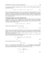
When the ordering decision is governed by the adjacent downstream stage, Table 2 shows
the optimal results of the independent approach, obtained using equations (44), (46) to (48)
with 3n = . Table 3 shows the results after sharing the coordination benefits, obtained using
equations (49) and (50). Detailed calculations to reach Tables 2 and 3 are also given in the
Appendix.

Stage Integer
multiplier
Cycle time

(year)
Cycle time
(days)
i
TC
∗
($ per
year)
Suppliers 1 0.09636 35.16 14,955.80

Manufacturers 3 0.09636 35.16 31,283.07
Retailers − 0.03212 11.72 18,677.85
Entire supply chain − − − 64,916.72
Table 2. Results for the decentralized model

Stage
Yearly
saving ($)
or penalty (−$)
Share
($ per year)
i
TC
D

($ per year)
Yearly cost
reduction (%)
Suppliers 1618.76 211.33 14,744.47 1.41

Manufacturers
−433.12
442.04 30,841.03 1.41
Retailers −268.35 263.92 18,413.93 1.41
Entire supply chain 917.29 917.29 63,999.43 1.41
Table 3. Results after sharing the coordination benefits
A Generalized Algebraic Model for Optimizing Inventory Decisions in a Centralized or
Decentralized Three-Stage Multi-Firm Supply Chain with Complete Backorders for Some Retailers

561
Table 3 shows that the centralized replenishment policy increases the costs of the four
manufacturers and six retailers, while decreases the cost of the two suppliers. According to
Goyal's (1976) saving-sharing scheme, the increased costs of the manufacturers and retailers
must be covered so as to motivate them to adopt the centralized replenishment policy, and
the total yearly saving of $917.29 is shared to assure equal yearly cost reduction of 1.41%
through all three stages or the entire chain.
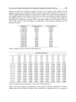
Because
33
18, 413.93 17,913.57TC TC
∗∗
=> =
D
, we have 1
χ
=
. Table 4 shows the adjusted
results, obtained using equations (52) and (53), and indicates that the retailers' yearly cost
reduction increases from 1.41% to 4.56% (which is rather significant), and the suppliers' and
manufacturers' yearly cost reductions are at least (
ii ii

ii
TC TC TC TC
TC TC
+∗
+∗
−−
≥
DD DD
because
, 1, 2
iii
TC TC TC i
+∗
≥≥ =
D
) 0.20% and 0.12%, respectively. However, if the retailers regard
0.49% as the relevant comparison figure and as insignificant, all the coordination benefit
may be allocated to them, and hence this figure becomes 0.85%
17,913.57 17,826.42 29.70 36.16
17,913.57
()
−++
=
.
If they consider 0.85% insignificant, negotiation between all the upstream stages and the
retailers is the last resort.

Stage
Adjusted share
($ per year)

i
TC
DD

($ per year)
Adjusted yearly
cost reduction (%)
Suppliers 29.70 14,926.10 0.20
Manufacturers 36.16 31,246.91 0.12
Retailers 851.43 17,826.42 4.56 (or 0.49)
Entire supply chain 917.29 63,999.43 1.41
Table 4. Results after adjusting the shares of the coordination benefits
The final remark for this example is that we need not assume that, for instance, supplier 1
supplies manufacturers 1 and 2, and supplier 2 supplies manufacturers 3 and 4. The mild
condition for a non-serial supply chain is to satisfy the equality:
123
123
111
JJJ
jjj
jjj
DDD
===
==
∑∑∑
.
7. Conclusions and future research
The main contribution of the chapter to the literature is threefold: First, we establish the n-
stage
(2, 3, 4,)n = " model, which is more pragmatic than that of Leung (2010b), by

including Assumption (13). Secondly, we derive expressions for sharing the coordination
benefits based on Goyal's (1976) scheme, and on a further sharing scheme. Thirdly, we
deduce and solve such special models as Leung (2009a, 2010a,b).
The limitation of our model manifest in the numerical example is that the number of
suppliers in Stage 1 is arbitrarily assigned. Concerning the issue of "How many suppliers are
best?", we can refer to Berger
et al. (2004), and Ruiz-Torres and Mahmoodi (2006, 2007) to
decide the optimal number of suppliers at the very beginning.
Three ready extensions of our model that warrant future research endeavors in this field are:
First, following the evolution of three-stage multi-firm supply chains shown in Section 3, we
can readily formulate and algebraically analyze the integrated model of a four- or higher-
stage multi-firm supply chain. In addition, a remark relating to determining optimal integral
Supply Chain Management

562
values of K's is as follows: To be more specific, letting 4n
=
, we have at most 6 (= 3×2×1)
options to determine the optimal values of
K
1
, K
2
and K
3
(see Leung 2009a, 2010a,b).
However, Option (1), evaluating in the order of
K
1
, K

2
and K
3
, might dominate other options
when the holding costs decrease from upstream to downstream firms. Although this
conjecture is confirmed by the numerical example in this chapter and those in Leung
(2010a,b), a formal analysis is still necessary.
Secondly, using complete and perfect squares, we can solve the integrated model of a
n-
stage multi-firm supply chain either for an equal-cycle-time, or an integer multiplier at each
stage, with not only a linear (see Leung 2010a) but also a fixed shortage cost for either the
complete, or a fixed ratio partial backordering allowed for some/all downstream firms (i.e.
retailers), and with lot streaming allowed for some/all upstream firms (i.e. suppliers,
manufacturers and assemblers).
Thirdly, severity of green issues gives rise to consider integrated deteriorating production-
inventory models incorporating the factor of environmental consciousness such as Yu
at al.
(2008), Chung and Wee (2008), and Wee and Chung (2009). Rework, a means to reduce
waste disposal, is examined in Chiu
et al. (2006) or Leung (2009b) who derived the optimal
expressions for an EPQ model with complete backorders, a random proportion of
defectives, and an immediate imperfect rework process while Cárdenas-Barrón (2008)
derived those for an EPQ model with no shortages, a fixed proportion of defectives, and an
immediate or a
N-cycle perfect rework process. Reuse, another means to reduce waste
disposal, is investigated in El Saadany and Jaber (2008), and Jaber and Rosen (2008).
Incorporating rework or reuse in our model will be a challenging piece of future research.
Appendix
A1. Derivation of equations (32) and (33)
Substituting equation (29) in the two conditions of (30) yields the following inequality

12
21
11 11
(1) (1)
H
H
KK KK
α
α
−
<< +.

We can derive a closed-form expression concerning the optimal integer
(1)
1
K
∗
as follows:

12
21
11 11
( 1) 0.25 0.25 ( 1) 0.25
H
H
KK KK
α
α
−+ < + < ++
12

21
22
11
( 0.5) 0.25 ( 0.5)
H
H
KK
α
α
⇔− < + <+


12
21
11
0.5 0.25 0.5
H
H
KK
α
α
⇔−< + <+


12 12
21 21
1
0.25 0.5 0.25 0.5
HH
HH

K
αα
αα
⇔+−≤<++.

From the last inequality, we can deduce that the optimal integer
(1)
1
K
∗
is represented by
expression (32). In an analogous manner, the optimal integer
(1)
2
K
∗
represented by
expression (33) is derived.
A Generalized Algebraic Model for Optimizing Inventory Decisions in a Centralized or
Decentralized Three-Stage Multi-Firm Supply Chain with Complete Backorders for Some Retailers

563
A2. Detailed calculations for the numerical example
Designations (2) to (13) give
1
11
3
ϕ
=
,

12
0.5
ϕ
= ,
21
0.5
ϕ
= ,
1
22
3
ϕ
=
,
23
0.25
ϕ
= ,
24
0.2
ϕ
= ,
1
1150 80 1230
α
=+=,
2
1200 203 7 1410
α
=++=,

3
300 32 332
α
=+=,
3
50 56 70 45 48 30 299
β
=
+++++= ,
0
0G
≡
,
12
1
33
100,000(0.8) 80,000(0.75)( ) 100,000G =− + − =− ,
2
70,000(2)(0.5 0.5) 50,000(2.1) 40,000(1.8) 20,000(2.2)(0.2 0.8) 203,400G =−−−+ −=−,
1
1
3
100,000( 0.88 0.8) 80,000(0.5 0.09 0.5 0.75) 142,933.33H =×++ ×+×= ,
1
2
3
70,000(0.5 0.83 0.5 2) 50,000( 2.91 2.1) 40,000(0.25 2.59 1.8) 20,000(0.2 0.85 0.8 2.2)
100,000 99,050 153,500 97,900 38,600 100,000 289,050,
H =×+×+×++ ×++×+×
−=+++−=

40,000(3.5)(5) 30,000(5.3)(5.1) 20,000(4.8)(4.8) 35,000(5.3)(4.9)
(b)
3
3.55 5.35.1 4.84.8 5.34.9
45,000(5.2) 10,000(5) 203, 400 378,036.84H
++ + +
=+ + + + +−= .

Equations (32), (33) and (26) give
1230(289,050)
(1)
1
1410(142,933.33)
0.25 0.5 1.92 1K
∗
⎢⎥
=
++= =
⎢⎥
⎣⎦
⎢⎥
⎣⎦
,
1230
1
378,036.84( 1410)
(1)
2
332(142,933.33 1 289,050)

0.25 0.5 3.18 3K
+
∗
×+
⎢⎥
=
++= =
⎢⎥
⎣⎦
⎢⎥
⎣⎦
,
1230 1410
33
(1, 3) 2( 332)(142,933.33 3 289,050 3 378,036.84) 299JTC =++ ×+ ×+ +
D


2(1212)(1,673,986.83) 299 $63,999.42=+=
per year.

Equations (34), (35) and (26) give
1410(378,036.84)
(2)
2
332(289,050)
0.25 0.5 2.91 2K
∗
⎢⎥
=

++= =
⎢⎥
⎣⎦
⎢⎥
⎣⎦
,
378,036.84
2
1230(289,050 )
(2)
1
142,933.33(1410 332 2)
0.25 0.5 1.99 1K
+
∗
+×
⎢⎥
=
++= =
⎢⎥
⎢⎥
⎣⎦
⎣⎦
,
1230 1410
22
(1, 2) 2( 332)(142,933.33 2 289,050 2 378,036.84) 299JTC =++ ×+ ×+ +
D

2(1652)(1,242,003.50) 299 $64,358.19=+=
per year.
Supply Chain Management

564
Hence, the optimal integral values of K
1
and K
2
are 1 and 3, and equations (24) and (25) give
the optimal basic cycle time and backordering times:
2(1212)
3
1,673,986.83
(1, 3) 0.03805
y
ear 13.89 da
y
sTT
∗
≡= = ≅
D
,
5(0.03805)
11
3.5 5
(1, 3) 0.02238
y
ear 8.17 da
y

stt
∗
+
≡= = ≅
D
,
5.1(0.03805)
22
5.3 5.1
(1, 3) 0.01866
y
ear 6.81 da
y
stt
∗
+
≡= = ≅
D
,
4.8(0.03805)
33
4.8 4.8
(1, 3) 0.01903
y
ear 6.95 da
y
stt
∗
+
≡= = ≅

D
,
4.9(0.03805)
44
5.3 4.9
(1, 3) 0.01828
y
ear 6.67 da
y
stt
∗
+
≡= = ≅
D
,
55
(1, 3) 0.03805
y
ear 13.89 da
y
stt
∗
≡= ≅
D
(all backorders),
66
(1, 3) 0tt
∗
≡
=

D
(no backorders).
The three yearly costs are obtained using equations (18) to (20) as follows:
2
142,933.33(1)(3)(0.03805) 100,000(3)(0.03805)
1150 80
7
1
2 2 1(3)(0.03805) 3(0.03805)
1
50 $13,337.04
j
j
TC
+
=
=−+++=
∑
per year,
4
(289,050 100,000)(3)(0.03805) 203,400(0.03805)
1200 203 32
2
2 2 3(0.03805) 0.03805
1
249 $31,716.19
j
j
TC
+

+
=
=−+++=
∑
per year,
6
(378,036.84 203,400)(0.03805)
300
3
2 0.03805
1
$18,946.20
j
j
TC
+
=
=+=
∑
per year.

In particular, the optimal solution to the model based on the equal-cycle-time coordination
mechanism is as follows:

(1, 1) 2(1230 1410 332)(142,933.33 289,050 378,036.84) 299JTC =++ ++ +
D

2(2972)(810,020.17) 299=+ $69,687.47
=
per year,

which is 8.89%
69,687.47 63,999.42
63,999.42
()
−
= higher than
3
(1, 3)JTC JTC
∗
≡
D
,
2(2972)
810,020.17
(1, 1) 0.08566
y
ear 31.27 da
y
sT == ≅
D
.

When the ordering decision is governed by the adjacent downstream stage, equations (44)
and (46) with 3
n = give
A Generalized Algebraic Model for Optimizing Inventory Decisions in a Centralized or
Decentralized Three-Stage Multi-Firm Supply Chain with Complete Backorders for Some Retailers

565

2(300)
3
378,036.84 203,400
0.03212 year 11.72 days
τ
∗
+
==≅
,
2
2(1200 203)
2
(289,050 100,000)(0.03212)
0.25 0.5 3.19 3
λ
+
∗
+
⎢⎥
=
++= =
⎢⎥
⎣⎦
⎢⎥
⎣⎦
,
2
2(1150 80)
1
142,933.33(3 0.03212)

0.25 0.5 1.95 1
λ
+
∗
×
⎢⎥
=
++= =
⎢⎥
⎣⎦
⎢⎥
⎣⎦
.

The three yearly costs are obtained using equations (47) and (48) with 3n
=
as follows:
3
2(300)(378,036.84 203,400) $18,677.85TC
∗
=+= per year,
(289,050 100,000)(3)(0.03212) 203,400(0.03212)
1200 203 32
2
2 2 3(0.03212) 0.03212
249 $31,283.07TC
+
∗
+
=−+++= per year,

142,933.33(1)(3)(0.03212) 100,000(3)(0.03212)
1150 80
7
1
2 2 1(3)(0.03212) 3(0.03212)
50 $14,955.80TC
∗
+
=−+++= per year.

The results for the decentralized model are summarized in Table 2, and the results after
sharing the coordination benefits are summarized in Table 3, in which columns 3 and 4 are
obtained using equations (49) and (50), respectively.
8. References
Banerjee, A., 1986. A joint economic-lot-size model for purchaser and vendor. Decision
Sciences 17 (3), 292-311.
Ben-Daya, M., Al-Nassar, A., 2008. An integrated inventory production system in a three-
layer supply chain. Production Planning and Control 19 (2), 97-104.
Ben-Daya, M., Darwish, M., Ertogral, K., 2008. The joint economic lot sizing problem: review
and extensions. European Journal of Operational Research 185 (2), 726-742.
Berger, P.D., Gerstenfeld, A., Zeng, Z.A., 2004. How many suppliers are best? A decision-
analysis approach. Omega 32 (1), 9-15.
Bhatnagar, R., Chandra, P., Goyal, S.K., 1993. Models for multi-plant coordination. European
Journal of Operational Research 67 (2), 141-160.
Cárdenas-Barrón, L.E., 2001. The economic production quantity (EPQ) with shortage
derived algebraically. International Journal of Production Economics 70 (3), 289-
292.
Cárdenas-Barrón, L.E., 2007. Optimal inventory decisions in a multi-stage multi-customer
supply chain: a note. Transportation Research Part E: Logistics and Transportation
Review 43 (5), 647-654.

Cárdenas-Barrón, L.E., 2008. Optimal manufacturing batch size with rework in a single-
stage production system: a simple derivation. Computers and Industrial
Engineering 55 (4), 758-765.
Cha, B.C., Moon, I.K., Park, J.H., 2008. The joint replenishment and delivery scheduling of
the one-warehouse,
n-retailer system. Transportation Research Part E: Logistics and
Transportation Review 44 (5), 720-730.
Supply Chain Management

566
Chan, C.K., Kingsman, B.G., 2007. Coordination in a single-vendor multi-buyer supply chain
by synchronizing delivery and production cycles. Transportation Research Part E:
Logistics and Transportation Review 43 (2), 90-111.
Chiou, C.C., Yao, M.J., Tsai, J.T., 2007. A mutually beneficial coordination mechanism for a
one-supplier multi-retailers supply chain. International Journal of Production
Economics 108 (1-2), 314-328.
Chiu, Y.S.P., Lin, H.D., Cheng, F.T., 2006. Technical note: Optimal production lot sizing with
backlogging, random defective rate, and rework derived without derivatives.
Proceedings of the Institution of Mechanical Engineers Part B: Journal of
Engineering Manufacture 220 (9), 1559-1563.
Chung, C.J., Wee, H.M., 2007. Optimizing the economic lot size of a three-stage supply chain
with backordered derived without derivatives. European Journal of Operational
Research 183 (2), 933-943.
Chung, C.J., Wee, H.M., 2008. Green-component life-cycle value on design and reverse
manufacturing in semi-closed supply chain. International Journal of Production
Economics 113 (2), 528-545.
El Saadany, A.M.A., Jaber, M.Y., 2008. The EOQ repair and waste disposal model with
switching costs. Computers and Industrial Engineering 55 (1), 219-233.
Goyal, S.K., 1976. An integrated inventory model for a single supplier single customer
problem. International Journal of Production Research 15 (1), 107-111.

Goyal, S.K., 1988. "A joint economic-lot-size model for purchaser and vendor": a comment.
Decision Sciences 19 (1), 236-241.
Goyal, S.K., Gupta, Y.P., 1989. Integrated inventory models: the buyer-vendor coordination.
European Journal of Operational Research 41 (3), 261-269.
Goyal, S.K., Deshmukh, S.G., 1992. Integrated procurement-production systems: a review.
European Journal of Operational Research 62 (1), 1-10.
Grubbstrom,

R.W., 1995. Modeling production opportunities: an historical overview.
International Journal of Production Economics 41 (1-3), 1-14.
Grubbstrom,

R.W., Erdem, A., 1999. The EOQ with backlogging derived without
derivatives. International Journal of Production Economics 59 (1-3), 529-530.
Hill, R.M., 1997. The single-vendor single-buyer integrated production-inventory model
with a generalized policy. European Journal of Operational Research 97 (3), 493-
499.
Jaber, M.Y., Rosen, M.A., 2008. The economic order quantity repair and waste disposal
model with entropy cost. European Journal of Operational Research 188 (1), 109-
120.
Joglekar, P.N., 1988. Comments on "A quantity discount pricing model to increase vendor
profits". Management Science 34 (11), 1391-1398.
Khouja, M., 2003. Optimizing inventory decisions in a multi-stage multi-customer supply
chain. Transportation Research Part E: Logistics and Transportation Review 39 (3),
193-208.
Leng, M.M., Parlar, M., 2009a. Lead-time reduction in a two-level supply chain: non-
cooperative equilibria vs. coordination with a profit-sharing contract. International
Journal of Production Economics. 118 (2), 521-544.
A Generalized Algebraic Model for Optimizing Inventory Decisions in a Centralized or
Decentralized Three-Stage Multi-Firm Supply Chain with Complete Backorders for Some Retailers

567
Leng, M.M., Parlar, M., 2009b. Allocation of cost savings in a three-level supply chain with
demand information sharing: a cooperative game approach. Operations Research
57 (1), 200-213.
Leng, M.M., Zhu, A., 2009. Side-payment contracts in two-person non-zero supply chain
games: review, discussion and applications. European Journal of Operational
Research 196 (2), 600-618.
Leung, K.N.F., 2008a. Technical note: A use of the complete squares method to solve and
analyze a quadratic objective function with two decision variables exemplified via a
deterministic inventory model with a mixture of backorders and lost sales.
International Journal of Production Economics 113 (1), 275-281.
Leung, K.N.F., 2008b. Using the complete squares method to analyze a lot size model when
the quantity backordered and the quantity received are both uncertain. European
Journal of Operational Research 187 (1), 19-30.
Leung, K.N.F., 2009a. A technical note on "Optimizing inventory decisions in a multi-stage
multi-customer supply chain". Transportation Research Part E: Logistics and
Transportation Review 45 (4), 572-582.
Leung, K.N.F., 2009b. A technical note on "Optimal production lot sizing with backlogging,
random defective rate, and rework derived without derivatives". Proceedings of the
Institution of Mechanical Engineers Part B: Journal of Engineering Manufacture 223
(8), 1081-1084.
Leung, K.N.F., 2010a. An integrated production-inventory system in a multi-stage multi-
firm supply chain. Transportation Research Part E: Logistics and Transportation
Review 46 (1), 32-48.
Leung, K.N.F., 2010b. A generalized algebraic model for optimizing inventory decisions in a
centralized or decentralized multi-stage multi-firm supply chain. Transportation
Research Part E: Logistics and Transportation Review 46 (6), 896-912.
Lu, L., 1995. A one-vendor multi-buyer integrated inventory model. European Journal of
Operational Research 81 (2), 312-323.

Maloni, M.J., Benton, W.C., 1997. Supply chain partnerships: opportunities for operations
research. European Journal of Operational Research 101 (3), 419-429.
Moore L.J., Lee S.M., Taylor B.W., 1993. Management Science. Allyn and Bacon, Boston.
Rosenblatt, M.J., Lee, H.L., 1985. Improving profitability with quantity discounts under
fixed demand. IIE Transactions 17 (4), 388-395.
Ruiz-Torres, A.J., Mahmoodi, F., 2006. A supplier allocation model considering delivery
failure, maintenance and supplier cycle costs. International Journal of Production
Economics 103 (2), 755-766.
Ruiz-Torres, A.J., Mahmoodi, F., 2007. The optimal number of suppliers considering the
costs of individual supplier failure. Omega 35 (1), 104-115.
Sarmah, S.P., Acharya, D., Goyal, S.K., 2006. Buyer vendor coordination models in supply
chain management. European Journal of Operational Research 175 (1), 1-15.
Seliaman, M.E., Ahmad, A.R., 2009. A generalized algebraic model for optimizing inventory
decisions in a multi-stage complex supply chain. Transportation Research Part E:
Logistics and Transportation Review 45 (3), 409-418.
Silver E.A., Pyke D.F., Peterson, R., 1998. Inventory Management and Production Planning
and Scheduling (3rd Edition). Wiley, New York.
Supply Chain Management

568
Sphicas, G.P., 2006. EOQ and EPQ with linear and fixed backorder costs: Two cases
identified and models analyzed without calculus. International Journal of
Production Economics 100 (1), 59-64.
Sucky, E., 2005. Inventory management in supply chains: a bargaining problem.
International Journal of Production Economics 93-94 (1-6), 253-262.
Wee, H.M., Chung, C.J., 2007. A note on the economic lot size of the integrated vendor-
buyer inventory system derived without derivatives. European Journal of
Operational Research 177 (2), 1289-1293.
Wee, H.M., Chung, C.J., 2009. Optimizing replenishment policy for an integrated production
inventory deteriorating model considering green component-value design and

remanufacturing. International Journal of Production Research 47 (5), 1343-1368.
Wu, K.S., Ouyang, L.Y., 2003. An integrated single-vendor single-buyer inventory system
with shortage derived algebraically. Production Planning and Control 14 (6), 555-
561.
Yang, P.C., Wee, H.M., 2002. The economic lot size of the integrated vendor-buyer inventory
system derived without derivatives. Optimal Control Applications and Methods 23
(3), 163-169.
Yu, C.P.J., Wee, H.M., Wang, K.J., 2008. Supply chain partnership for three-echelon
deteriorating inventory model. Journal of Industrial and Management
Optimization 4 (4), 827-842.
27
Life Cycle Costing, a View of Potential
Applications: from Cost Management Tool to
Eco-Efficiency Measurement
Francesco Testa
1
, Fabio Iraldo
1,2
, Marco Frey
1,2
and

Ryan O’Connor
2

1
Sant’Anna School of Advanced Studies, Piazza Martiri della Libertà 33, 56127 Pisa,
2
IEFE – Institute for Environmental and Energy Policy and Economics,
Via Roentgen 1, 20136, Milano

Italy
1. Introduction
In the field of modern production contexts, the complexity of processes combined with an
increasingly dynamic competitive environment has created, in business management, the
need to monitor and analyze, in terms of generation costs, not only the internal production
phase but all stages both upstream and downstream in order to minimize the total cost of
the product throughout the entire life cycle.
The approach of life-cycle cost analysis was used primarily as a tool to support investment
decisions and complex projects in the field of defence, transportation, the construction sector
and other applications where cost constitutes the strategic analysis of cost components of a
project throughout its useful life.
The analysis methodology of Life Cycle Costing (LCC) concerns the estimate of the cost in
monetary terms, originated in all phases of the life of a work, i.e. construction, operation,
maintenance and eventual disposal / recovery. The aim is to minimize the combined costs
associated with each phase of the life cycle, appropriately discounted, thus providing
economic benefits to both the producer and the end user.
Life Cycle Costing (LCC) is a tool used in consolidated management accounting (Horngren,
2003, Atkinson et al., 2002), which aims to achieve a reduction in carbon dioxide. Whole life
cost. This identifies, with reference to the system, the functional activities within the
appropriate stages of design, production, use and disposal of waste, and appropriates a cost
(Fabricky Blanchard, 1991) in order to clarify the causal relationship between resulting
architecture of product design alternatives and cost estimates of fees, which will probably be
supported by the various actors within the economic life of the product [Fixson, 2004].
Life Cycle Costing is an analytical tool and method which belongs to the set of life cycle
approach. Traditionally, LCC was used to support purchasing decisions of products or
capital equipment involving a large outlay of financial resources (Huppes et al., 2005). In the
definition provided by Rebitzer & Hunkeler (2005) LCC incorporates all costs, both internal
and external, associated with the life cycle of a product, and are directly related to one or
more actors in the supply chain.
Supply Chain Management

570
In recent years, the spread of life cycle thinking within business planning and management
has led to an evolution of LCC methodology by extending the scope of integrated analysis of
the three pillars comprising sustainable development - economic, environmental and social
– in a financial representation.
Analysis of different applications undertaken in recent years identifies three types of Life
Cycle Costing, for separate purposes and methods of application: Business LCC,
Environmental LCC and Social LCC.
Business LCC, or traditional LCC, is commonly used as a method of cost analysis and
business decision support in procurement and investment. Cost categories and principles
that are to be followed in the measurement procedure need to be established in advance,
and the functional unit is represented by just one product.
Environmental LCC in the product or system under study is usually less complex and the
functional unit is chosen according to international standards as specified by ISO 14040 (i.e.
1m² of floor). Unlike the traditional LCC, it is not used as a tool for procurement decisions or
control, but to analyze the environmental and economic impact of a product or system. The
cost estimate is obviously simpler than what occurs in the traditional LCC approach and is
usually characterized by a static (steady state). In Environmental LCC, the integration of the
instrument in Life Cycle Assessment is one of the fundamental aspects.
The Social LCC is the third component of the measure of sustainable development, in
addition to the LCA and Environmental LCC (Hunkeler et al., 2006). The goal is to allow the
organization to conduct its business in a responsible manner by providing information on
potential social impacts caused to individuals by the product during its life cycle.
The analysis of social impacts, as is the case for environmental LCC, takes into account both
the internal and external costs. Internal costs are those that the various actors involved
during the lifecycle of a product must support, such as production costs or the costs of use;
while the external costs, also called externalities, are related to the effects of monetized
environmental and social impacts generated by a given product. These costs are usually not
directly borne by the consumer or derived from making or using the product, but affect the

entire community indiscriminately.
The following chapter will highlight the main applications of Life Cycle Costing
methodology, both as a tool for minimizing business costs for a project or a product and as
an essential component of sustainability-oriented life cycle management. In the final section,
we will see a short description of the possible application of LCC for the construction of eco-
efficiency indicators
2. Business life cycle costing
The issue of life cycle costing arrives in the context of at least two aspects: one related to the
development of new products, the other in the evaluation of strategic investments (Ciroth,
2003).
The first refers to the application of Life Cycle Costing to identify, measure and evaluate the
costs associated with the entire life cycle of a new product, especially in the case of complex
and durable products. The second concerns the application of LCC as a tool for comparative
analysis of long-term investment projects and in managing the cost of a new product.
The application of LCC in the management of the product can be seen from two distinct
perspectives:
Life Cycle Costing, a View of Potential Applications:
from Cost Management Tool to Eco-Efficiency Measurement

571
1. From the economic perspective of a producer, to support management in planning and
managing the product throughout its life cycle;
2. From the economic perspective of a customer, or as an aid in the purchasing stage
aimed at determining the total cost for the entire life cycle.
From the perspective of the producer, calculations consist of the estimation of the costs of
design, engineering, industrialization and production of a new product and in the analysis
of these costs throughout the life cycle (Asiedu & Gu, 1998).
Once the life cycle duration of the product has been identified and individual cost elements
produced in the various stages has been identified and measured, a detailed analysis can
highlight the relationships between the individual cost items of each phase.

The decisions taken during planning and design can have an impact on the costs incurred in
subsequent phases. An example can be durable consumer goods, such as appliances: the
choice between different technological solutions in the design phase can strongly influence
the efficiency of the product and thus reduce or increase its usage cost. Efficiency measures
the relation between outputs from and inputs to a process, the higher the output for a given
input, or the lower the input for a given output, the more efficient is an activity, product, or


Source: Vitali, 2004 (adapted from Susman, 1995)
Fig. 1. The life cycle of a product
Supply Chain Management

572
business (Burritt & Saka 2006). The traditional cost accounting systems tend to focus on the
production phase, underestimating the importance of cost information relating to upstream
and downstream stages. An integrated view of the different phases of the lifecycle, however,
show that the maximization of value added does not depend strictly on cost minimization or
revenue maximization at each stage.
Following the product throughout its life cycle ensures a useful flow of information to all
business functions regarding the elements that determine the success of a product, allowing
them to react promptly and effectively to resolve any weaknesses. From this perspective,
Life Cycle Costing moves from a mere trend costing instrument to assuming a key role in
the support strategies and decisions of business management.
From the perspective of the customer, the LCC aspect of the concept of Total Cost of
Ownership (TCO) is defined as a philosophy of cost calculation aimed at determining the

total cost of purchase, possession and use of a particular product (Ellram, 1995). This
philosophy recognizes that the purchase price represents only one component of the total
cost of a product throughout its useful life and can be applied both to the process of
purchasing goods and as a capital investment tool by organisations (Ellram & Sifred, 1998).

TCO, compared to traditional methods of cost analysis of the life cycle, has some distinctive
features: the range of costs considered is wider considering the cost of the first purchase.
Moreover, while LCC considers only the costs as quantifiable monetary values, TCO also
extends to the costs associated with the low quality of a product and related services, and all
the opportunity costs associated with such low quality (Pitzalis, 2003b).
A survey of consumers conducted in the 1970’s by Hutton and Wilkie found that consumers
who make buying decisions using the LCC approach could lead to a reduction in the
consumption of energy equal to a saving of $ 4 billion annually (Hutton and Wilkie, 1980).
The use of LCC in the procurement phase is also desirable from the economic perspective of
the buyer. Taking Italy as an example, we find that the volume of public spending of Public
Administration represents 17% of the Gross Domestic Product (GDP), compared to 18% on
average in the EU, and 15% in the USA (Iraldo et al. 2008).
A survey conducted by ICLEI - Local Governments for Sustainability - in 2007 on behalf of
the European Commission, shows how the use of LCC during purchasing would allow, for
certain types of products, financial savings as well as offering significant environmental
benefits.
3. The product lifecycle and Life Cycle Assessment (LCA)
In recent years, different methodologies have been developed as a direct response to
increasing environmental threats, in order to study and evaluate the environmental impacts
associated with a product. The need to develop operational and technical management tools
in this area is gained as a result of a more environmental focus and mounting pressure from
external partners of the undertaking, who increasingly request guarantees regarding the
environmental compatibility of products. In order to address these challenges,
environmental considerations need to be integrated into a number of different types of
decisions made both by business, individuals, and public administrations and policymakers
(Nilsson and Eckerberg, 2007) This has prompted companies, scientific institutions and
standardisation bodies (national and international) to study, develop and progressively
refine methodologies that would respond to the needs of public authorities, business
partners, consumers and, more generally, by all stakeholders of an organisation.
Life Cycle Costing, a View of Potential Applications:

from Cost Management Tool to Eco-Efficiency Measurement

573
The first problem we find in the definition of methodological tools of environmental
assessment is the correct measurement of the impacts as related to a product. It is known
that a product passes through different stages during its lifetime: from the initial
manufacture through the process of production, consumption throughout the use of the
product, and finally the “death” (and disposal) with the exhaustion of its function. During
each of these stages, the product has a number of impacts on the environment. The
significance of these impacts may vary depending on the stage of the lifecycle that is treated;
if the study of the impact, for example, is limited to a single phase, the outcome could be
misleading. The main tool, available to scholars to conduct an examination congruent with
the requirements mentioned, is the method known as "Life Cycle Assessment". This tool,
developed to overcome these potential drawbacks, has as its focal point the performance
analysis of systems, applied to assess the potential environmental impacts and resources
used throughout a product’s lifecycle, i.e., from raw material acquisition, via production and
use phases, to waste management (ISO, 2006a).
This approach is also defined as "cradle to grave". The comprehensive scope of LCA is
useful in order to avoid problem-shifting, for example, from one phase of the life-cycle to
another, from one region to another, or from one environmental problem to another
(Finnveden et al 2009).
LCA-methodology and the term was first coined during a SETAC (Society of Environmental
Toxicology and Chemistry) conference in 1990 in Vermont (USA), and is defined as "an
objective process of evaluation of environmental burdens associated with a product ( )
through identifying and quantifying energy and materials used and waste released into the
environment, to assess the impact of these uses of energy and materials and releases into the
environment and to evaluate and implement environmental improvement opportunities.
The assessment includes the entire lifecycle of the product ( ), including extraction and
processing of raw materials, manufacture, transport, distribution, use, reuse, recycling and
final disposal" ( SETAC, 1993).

The first LCA studies were undertaken in the late sixties and covered some aspects of the
life cycle of materials and products, to highlight issues such as energy efficiency,
consumption of raw materials and waste disposal. Starting from these early experiences,
there has been a gradual spread of use of such means, promoted by the positive results that
first applications produced. Simultaneously, however, there were obvious limits to this
methodology due, mainly, to the non-comparability of results, owing to the development
with different approaches and methodologies [Baldo, 2000]. To fill this gap, in the 1990s,
efforts were made by standardisation bodies at national and international levels, aiming to
rationalize and harmonize the references in this field.
The development of LCA methodology culminated in the codification of a family of
standards, ISO 14040 (Environmental Management - Life cycle assessment), published in
1997. Today the ISO 14040 constitutes the most important reference for the dissemination of
these methodologies. The provision recognizes the LCA tool utility in identifying
opportunities for improving the environmental aspects of product in the various stages of
the lifecycle, in identifying the most appropriate indicators for measuring the environmental
performance, guiding the design of new products/processes in order to minimise its
environmental impact and strategic planning in support of businesses and policy maker
(ISO, 1996). In this logic, LCA is also used as the basis of scientific information
communication strategies of organisations, that is, in the definition of instruments that can
Supply Chain Management

574
be used for this purpose, such as those assertions of type II (environmental product
declarations) or of type I (eco-labelling programmes). The European ecolabel, for example,
utilises LCA for processing of ecological criteria and environmental product statements are
to be assured by the results of a life cycle analysis, according to the specifications in ISO
14025.
There exists a wealth of data and methods for LCA throughout the world today, with
government bodies and international organisations recognising that there is an increasing
need for guidance on what to use. The UNEP/SETAC Life Cycle Initiative is an example of

one of the international activities underway to disseminate life cycle approaches throughout
the world, with a focus on developing countries (UNEP 2002). The life cycle initiative and
other related life cycle activities, such as the International Reference Life Cycle Data System
(ILCD) (European Commission 2008) are instrumental in expanding LCA approaches and in
supporting the increasing understanding and application of life cycle assessments. In this
way, the expansion of LCA is an approach based on expanding the usefulness of LCA whilst
not increasing the complexity of the LCA, thereby decreasing it’s value.
According to ISO, LCA is a technique for assessing the environmental aspects and potential
impacts throughout the life cycle of a product or process or service, which is divided into
four phases (see the figure 2):
1. Setting the goals and boundaries of the system (goal and scope definition - ISO 14041)
2. Data collection (inventory analysis - ISO 14041);
3. Environmental impact assessment (impact assessment - ISO 14042);
4. Interpretation of results and improvement (improvement analysis - ISO 14043).
The 4 phases of LCA should not be seen as a fixed sequence or standard of methodological
steps, but rather as a cycle of iterations, with frequent changes and revisions of the contents
of each, as each phase is interdependent with others.
1) The first stage indicates clearly and coherently the planned application, the reasons why
the LCA is developed, the intended use of the results and the intended audience of the
study. In particular, in defining the scope of the study, certain elements must be clearly


Fig. 2. The phases of LCA
Life Cycle Costing, a View of Potential Applications:
from Cost Management Tool to Eco-Efficiency Measurement

575
described and taken into account, including: the functions of the product system (or systems
product in the case of comparative studies, as LCA can be used to compare the alternative
products or processes); the functional unit; the system of the product (defined in the

standard as "the set of elementary units of the combined process with regard to the matter
and energy, pursuing one or more defined function"); the types of impacts, methodologies
for evaluating the impact and the subsequent interpretation to be used; the quality
requirements of initial data, etc.
Within this phase, a fundamental step is the definition of the functional unit, whose purpose
is to provide a reference in which to bind the inflows and outflows (defined as inflows of
matter or energy that enters a process unit consisting of raw materials or products, and
outflow matter or energy that leaves a unit process, formed from raw materials,
intermediate products, products, emissions or waste), as we assume that the measures and
evaluations are conducted according to the provision of the system under consideration. In
other words, the system covered by the study is the product, defined not so much by its
physical characteristics, as in its function, i.e. in the service that it provides (European
Environmental Agency, 1998). If the function performed by the painting of a steel artifact,
for example, is the protection of atmospheric corrosion, the functional unit could be defined
as the unit of area protected to a predetermined period of time.
Another key step in conducting a LCA study is the definition of borders of the system
studied, namely the identification of individual operations (units) that make up the process
and their inputs and outputs, which must be included in the study. All transactions, or
"process units", within the confines of the system are interrelated: they receive their input
from the unit "upstream" while their output constitutes the inputs of “downstream” units,
according to the outline of the process studied.
The criteria used to define the boundaries must always be identified and justified in order to
clearly spell out the scope of the study.
2) The successive step in the undertaking of LCA’s is the lifecycle inventory phase (LCI).
This phase involves collecting data and calculation procedures that enable the quantification
of the types of interaction that the system has with the environment; these interactions may
cover the use of resources and emissions in the air, the releases into water or soil associated
with the system-product (Frankl, Rubik, 2000). The process of how to conduct an analysis is
iterative in nature: inventory or data collection allows an increased level of knowledge of
the system and, consequently, new data requirements may emerge or new requirements or

limitations concerning data already collected may be identified. All this may entail a change
to collection procedures and methodologies for calculation, in order to maintain a study
coherent with objectives and allow, then, the achievement of a consistent audit. A review of
the purpose or scope of the study may also be demanded by the emergence of problems
related to the non-availability of required information. In relation to the latter issue, it
should be noted that recent years have been characterised by a strong development of
commercial and public databases both in the private and public domain. National or
regional databases, which evolved from publicly funded projects, provide inventory data on
a variety of products and basic services that are needed in every LCA, such as raw materials,
electricity generation, transport processes, and waste services as well as sometimes complex
products (Finnveden et al. 2009). In the private sector, as understanding grew of the
increasing importance that the LCA tool has in environmental strategies of enterprises, and
in public sector entities, in order to support enterprises in its application. This development