MIMO Systems Theory and Applications Part 6 doc

b) When r > t, then
C
=
r
∑
k=1
t
−1
∑
j=0
log
2
e
t
I
−k + 1 + j
+
log
2
e ·
∑
t
h
=1
| D(h) |
|V(Δ)|
(40)
where D
(h)=(d
i,j
(h)) is an r ×r matrix satisfying

d
i,j
(h)=
⎧
⎪
⎪
⎪
⎨
⎪
⎪
⎪
⎩
∑
j−1
k
=0
(−j+1)
k
(t−j+ 1)
k
δ
r−j+k
i
(t+t
I
−j+1)
k
k!
, j = h, j ≤ t
δ

r−j
i
, j = h, j > t
h
i,j
−(
∑
t−j
b
=0
1
t
I
+b
)
∑
j−1
k
=0
(−j+1)
k
(t−j+ 1)
k
δ
r−j+k
i
(t+t
I
−j+1)
k

k!
, j = h.
(41)
Here
h
i,j
= δ
r−j
i
Γ(t + t
I
− j + 1)
Γ(t
I
)Γ(t − j + 1)

1
0
x
t−j
(1 − x)
t
I
−1
(1 −δ
i
x)
j−1
[ln(1 −δ
i

x) −ln(1 − x)]dx. (42)
3.4 Numerical examples and remarks
Now we offer some numerical examples validating the analysis and showing the effect of
various system parameters on the ergodic capacity of MIMO systems. For simplicity, we adopt
the correlation model of exponential type (see [Loyka (2001)] and [Kiessling (2005)]) at the
receiver with
Σ
=[β
|i−j|
] (43)
Σ
I
=[β
|i−j|
I
] (44)
The correlation coefficients β and β
I
are for the desired user and interferers, respectively. They
range from 0 to 1. Here 0 means that the correlation is the weakest, and 1 means that the
correlation is the strongest. Furthermore, the SIR in dB is defined by 10 log
10

E
s
t
I
E
I


which
characterizes the signal to interference ratio in the considered physical condition.
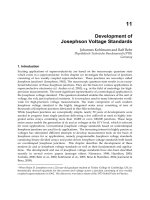
The ergodic capacity versus the SIR is depicted in Fig.1 where the four curves are shown for
four different correlation coefficients equal to β
= 0.3, 0.6, 0.8, 0.9, respectively. The considered
MIMO system possesses 4 transmit antennas and 4 receive antennas with 10 interfering
antennas. The correlation coefficient β
I
is set at 0.4. As expected, the ergodic capacity decreases
with increasing β. It can be further seen that the effect of strong correction on the capacity is
significant.
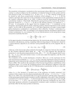
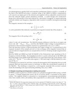
Fig.2 depicts the ergodic capacity versus the SIR for four different correlations. The four
curves in Fig.2 are shown for interfering correlation coefficients equal to β
I
= 0.3, 0.6, 0.8, 0.9,
respectively. The considered MIMO system is with 2 transmit antennas and 4 receive antennas
and interfered by a user with 8 antennas. The correlation coefficient is set at β
= 0.5. It can be
seen from Fig.2 that the impact of correlation for interferers on the ergodic capacity increases
with increased interfering correlation coefficient β
I
. Therefore, the interference correlation is
beneficial, especially the strong correlation.
Simulation results are included in Figs.1-2 for comparison. Each point in the simulation curves
are obtained by averaging over 100, 000 independent computer runs. The theoretical and
simulation results are nearly identical verifying the validity of the theory. Consequently, in
the following evaluations, we only consider the theoretical results.
164
MIMO Systems, Theory and Applications
−5 0 5 10 15 20 25 30

0
5
10
15
20
25
30
35
40
SIR (dB)
Ergodic Capacity (bit)


Theory results, β=0.3
Theory results, β=0.6
Theory results, β=0.8
Theory results, β=0.9
Monte−Carlo simulation results
Fig. 1. Ergodic capacity versus SIR for different signal channel correlations.
−5 0 5 10 15 20 25 30
0
5
10
15
20
25
30
SIR (dB)
Ergodic Capacity (bit)

Theory results, β
I
=0.3
Theory results, β
I
=0.6
Theory results, β
I
=0.8
Theory results, β
I
=0.9
Monte−Carlo simulation results
Fig. 2. Ergodic capacity versus SIR for different interfering correlations.
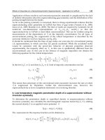
In Fig.3, a MIMO system with 4 transit antennas and 4 receive antennas is considered. We
assume only 1 interferer is involved in this system. We observe the ergodic capacities with
various interference antennas. In Fig.3, the four curves correspond to the number of total
interfering transmit antennas t
I
= 4, 5, 6, 7, respectively. It can be observed that the ergodic
capacity drops as t
I
increases, and the drop becomes gradually slow.
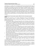
Finally, in Fig.4, we compare our analytical results (neglecting the noise component) with the
Monte-Carlo simulation results with Gaussian noise involved in the corresponding physical
conditions. We set the transmit power in the interest system at 30dB, and let β and β
I
be qual
to 0.4 and 0.8, respectively. Furthermore, we assume the system is interfered by a user with 10

antennas. We plot the curves with t
= r = 2, 3 and 4, respectively. As shown in the figure, our
165
Analysis of MIMO Systems in the Presence of Co-channel Interference and Spatial Correlation
−5 0 5 10 15 20 25 30
0
5
10
15
20
25
30
35
40
45
SIR (dB)
Ergodic Capacity (bit)


Theory results, t
I
=4
Theory results, t
I
=5
Theory results, t
I
=6
Theory results, t
I

=7
Fig. 3. Ergodic capacity versus SIR for various interfering antenna configurations.
−5 0 5 10 15 20 25 30
0
5
10
15
20
25
30
35
SIR (dB)
Ergodic Capacity (bit)


Theory results without noise, t=2,r=2
Theory results without noise, t=3,r=3
Theory results without noise, t=4,r=4
Monte−Carlo simulation results with noise
Fig. 4. Ergodic capacity versus SIR for various antenna configurations.
analytical results match the simulation results under low SIRs, however, we lose the precision
gradually as SIR grows.
4. Outage performance of TRD MIMO systems with interference and correlation
4.1 System model
Suppose the intended user employs r antennas to receive signals transmitted from t antennas.
The channels that link the t transmit and r receive antennas are characterized by an r
×t matrix
H, which is assumed to follow the joint complex Gaussian distribution with mean matrix M
166
MIMO Systems, Theory and Applications

and covariance matrix Σ ⊗Ψ. Symbolically, we will write
H
∼ CN
r,t
(M, Σ ⊗Ψ) (45)
where Ψ and Σ define the correlation structure at the transmit and receive ends, respectively.
It is assumed that the intended signal is corrupted by
 independent interferers, and the ith
interferer transmits its signal with t
i
antennas where i = 1, ,. The desired information
symbol b
0
is weighted by the transmit beamformer u before being feeded to the t transmit
antennas. The transmit beamformer is normalized to have a unit norm u
†
u = 1 so that the
transmit energy equals E
s
= |b
0
|
2
.Ther × 1 vector at the desired user’s receiver can thus be
written as
y
= b
0
Hu +


∑
i=1
H
i
s
i
+ n, (46)
where H
i
is the r × t
i
the channel matrix characterizing the links from the desired user’s r
receive antennas to the t
i
transmit antennas of interferer i;ands
i
is the symbols transmitted
by interferer i,suchthat
E[s
i
s
†
i
]=E
i
I
t
i
with E
i

denoting the average symbol energy. In the
way similar to defining H, we assume
H
i
∼ CN
r,t
i
(M
i
, Σ
i
⊗Ψ
i
) (47)
We assume the additive noise vector n to follow the r
× 1 complex Gaussian distribution of
mean zero and covariance matrix R
n
. Conditioned on H
i
, i = 1, ,, the covariance matrix
of interference-plus-noise component is given by
R
c
=

∑
i=1
E
i

H
i
H
†
i
+ R
n
. (48)
4.2 Formulation
The TRD system transmits one symbol at a time, and employs a weighting vector
w to combine received vector y to form a single decision variable. The transmit and
receive weighting vectors, u and w should be chosen to maximize the output signal to
interference-plus-noise ratio (SINR) at every time instant, as defined by
γ
=
w
†
(Hu)(Hu)
†
w
w
†
E
n

(
∑

i=1
H

i
s
i
+ n)(
∑

i=1
H
i
s
i
+ n)
†

w
(49)
where
E
n
denotes the expectation with respect to n. The result of expectation equals R
c
given in (48). Optimization of γ is the problem of Rayleigh quotient. Given the channel-state
information and conditional on u, we optimize γ with respect to w to obtain [Kang & Alouini
(2004b)]
γ
(u)=
u
†
(E
s

H
†
R
−1
c
H)u
u
†
u
(50)
where we have used the fact that u
†
u = 1 to represent the second line in the form of Rayleigh
quotient. Thus, we can upper bound γ
(u) by
γ
max
= λ
(1)
(51)
167
Analysis of MIMO Systems in the Presence of Co-channel Interference and Spatial Correlation
where λ
(1)
≥ λ
(2)
≥···λ
(q)
are the non-zero eigenvalues of the matrix product
F

= E
s
H
†
R
−1
c
H (52)
in the descending order, and v
(1)
, v
(2)
, ··· , v
(q)
are their corresponding eigenvectors.
The non-ordered eigenvalues and eigenvectors will be denoted by λ
1
, λ
2
, ··· , λ
q
and
v
1
, v
2
, ··· , v
q
, respectively.
The outage probability of TRD systems can be defined directly in terms of the instantaneous

SINR γ
max
= λ
(1)
or by channel capacity [Kang et al. (2003)]
C
= log
2
(1 + λ
(1)
). (53)
Both leads to the same expression for an outage event: λ
(1)
< Λ, but with the protection ratio
Λ defined differently as shown by
Λ
=

γ
0
, outage in terms of γ
2
C
0
−1, outage in terms of C.
(54)
In either case, we can write the outage probability as
P
out
= Pr{λ

(1)
< Λ}. (55)
To determine the outage performance, the central issue is to determine the probability density
function (PDF) of λ
(1)
or equivalently, its cumulative density function (CDF).
Determination of the CDF of the principal eigenvalue of a rank-q non-negative definite matrix
of the form F
= E
s
H
†
R
−1
c
H has been addressed intensively in the literature [Muirhead (1982)].
The predominant methodology, however, is to arrange the sample eigenvalues in a descending
order and then to determine the PDF of the largest one. The methodology is also prevailing
in the area of communications [Kang & Alouini (2004b)]. Such methodology, however, often
leads to mathematically intractability except for some simple cases. In this paper, we therefore
consider the non-ordered sample eigenvalues instead. The key step is to represent the outage
event λ
(1)
< Λ, alternatively, by virtue of non-ordered eigenvalues. To this end, we write the
sample space
{F : λ
(1)
< Λ)} = {F : ∩
q
i

=1
(
λ
i
< Λ
)
}
. (56)
The right-hand side is further expressible in matrix form. Hence,
{F : λ
(1)
< Λ} = {F : F < ΛI} (57)
where F
< ΛI means that (ΛI − F) is a positive definite matrix. The equivalence of the two
expressions is obvious, in much the same way as what we do in selection combining. Let V
denote the matrix of eigenvectors of F.Namely,V
=(v
1
, ··· , v
q
, ··· , v
t
). Hence we can write
ΛI
−F = Vdiag(Λ −λ
1
, ··· , Λ −λ
q
,0,···,0)V
†

(58)
The positive definiteness of
(ΛI −F) implies that all of eigenvalues Λ − λ
i
are positive, and
vice versa, thus showing the correctness of (57). This equivalence was previously used in
Chapter 9 of [Muirhead (1982)].
We use it here to represent the outage probability yielding
P
out
= Pr{F < ΛI}. (59)
168
MIMO Systems, Theory and Applications
The matrix representation of outage event, though simple in principle, provides a novel
framework to tackle the outage issue of the optimal TRD system. The key to success along
this direction is to find the joint cumulative distribution function of matrix F.
For ease of presentation, we define variables
u
= max{r, t} (60)
v
= min{r, t} (61)
and the v
×u complex matrix
Υ
=

Σ
−1/2
MΨ
−1/2

, r < t
Ψ
−1/2
M
†
Σ
−1/2
, t ≤ r.
(62)
4.3 Outage performance with co-channel interference
We first proceed to operational environments with co-channel interference. For mathematical
tractability, let us first simplify the interference covariance matrix given in (48). We assume
that the operating environment is interference-dominated, so that the noise component is
negligible. Hence, we can rewrite (48) as
R
c
=

∑
i=1
E
i
H
i
H
†
i
(63)
where H
i

H
†
i
∼ CW
r
(t
i
, Σ
i
). For the case with E
1
= E
2
= ···= E

= E
I
and Σ
1
= Σ
2
= ···=
Σ

= Σ
I
, it is easy to use Theorem 3.2.4 of Muirhead [Muirhead (1982)] to assert that R
c
,upto
a factor of E

I
, follows the Wishart distribution, as shown by
R
c
∼ CW
r
(t
I
, Σ
I
) (64)
where t
I
=
∑

i=1
t
i
. Clearly, this is the extension of the closure property of chi-square
distribution. For the general setting of E
i
’s, we can accurately approximate R
c
by using a single
Wishart-distributed matrix, say Q
1
, in much the same as what we do for a sum of chi-square
variables [Pearson & Hartley (1976)]. The resulting matrix Q
1

has the following distribution
Q
1
∼ CW
r
(t
1
, Σ
1
), (65)
for which the parameters t
1
and Σ
1
can be determined by equating the first two moments of
Q
1
and R
c
; for details, see Chapter 3 of [Gupta & Nagar (2000)]. From the above analysis, it
follows that we can use a single a Wishart-distributed matrix, say Q
1
,toreplaceR
c
to simplify
the analysis. It also follows that t
1
is usually much greater than the number of antennas of the
intended user. Thus, without loss of the generality, we can write the decision matrix (52) as
F

=(E
s
/E
1
)H
†
Q
−1
1
H (66)
whereby, for a given power protection ratio Λ, the outage probability can be written as
P
out
(x)=Pr{F < ΛI}
=
Pr{J < xI} (67)
169
Analysis of MIMO Systems in the Presence of Co-channel Interference and Spatial Correlation
where x = ΛE
1
/E
s
and J is defined in terms of random channel matrices H and Q
1
,asshown
by
J
= H
†
Q

−1
1
H. (68)
We assume the signal suffers from Rician fading so that the corresponding channel matrix
H
∼ CN
r,t
(M, Σ ⊗ Ψ). Suppose that the interferer employs t
1
transmit antennas such that
r
≤ t
1
. We also assume that the t
1
channel-gain vectors for the interferer that link each transmit
antenna to the r receive antennas are independent and identically distributed as CN
r
(0, Σ
1
).
Then, we can assert that Q
1
∼ CW
r
(t
1
, Σ
1
). Under these assumptions and by introducing the

following matrix notations:
Δ
=

Σ
−1
Σ
1
, t ≤ r
Ψ
−1
, r < t
(69)
and
Θ
=

Σ
−1
Σ
1
, r < t
Ψ
−1
, t ≤ r
(70)
we can explicitly work out the outage probability defined in (67), obtaining results
summarized in the following theorem. The proof of this theorem is placed in 7.1.
Theorem 3. The outage probability of the optimal TRD system with co-channel interference is given
by

P
out
(x)=d
∞
∑
k=0
x
uv+ k
k!
∑
κ
[t + t
1
]
κ
[u + v]
κ
P
κ
(Υ, Δ, Θ) (71)
where
d
=
˜
Γ
v
(t + t
1
)
˜

Γ
v
(v)
˜
Γ
v
(t + t
1
−u)
˜
Γ
v
(u + v)
|
Δ|
v
|Θ|
u
·etr[−ΥΥ
†
]
The above generalized Hermite polynomial P
κ
(·, ·, · ), though difficult in numerical calculation
[Gupta & Nagar (2000)], serve as a fundamental tool in the study of the distribution of some
quadratic forms. Eq.(71) is a general formula, providing a solid foundation for further study.
This combination can be treated as a special Rayleigh case by setting M
= 0.Namely,H ∼
CN
r,t

(0, Σ ⊗Ψ). With the condition, Theorem 3 leads to the following corollary.
Corollary 1. Let M
= 0.Then
P
out
(x)=d
1
x
uv
2
˜
F
(u,v)
1
(u, t + t
1
; u + v; xΔ, −Θ) (72)
where
d
1
=
∼
Γ
v
(t + t
1
)
∼
Γ
v

(v)
∼
Γ
v
(t + t
1
−u)
∼
Γ
v
(u + v)
|
Δ|
v
|Θ|
u
(73)
The corollary is made by inserting M
= 0 into (71) and invoking Property 9 in Section 2 (i.e.
the complex counterpart of Expression (1.8.3) in [Gupta & Nagar (2000)]).
Our concern is whether (72) can be further simplified. To this end, we note that when r
= t,the
hypergeometric function
2
˜
F
(u,v)
1
involved in (72) can be converted to scalar hypergeometric
functions which are much easier to calculate by using for example, the built-in functions in

Matlab, Mathematica and Maple. The simplification can be done by invoking the following
lemma (see Lemma 2 in [Kiessling (2005)]).
170
MIMO Systems, Theory and Applications
Lemma 2. Let A = eig(X)=diag(λ
1
, ,λ
p
) and B = eig(Y)=diag(ω
1
, ,ω
p
) with λ
1
>
> λ
p
and ω
1
> > ω
p
. Furthermore define
Γ
p
(p)=
p
∏
i=1
Γ(p −i + 1), (74)
α

p
(A)=
∏
i<j
(λ
i
−λ
j
) (75)
and
Ψ
p
n
(b)=
p
∏
i=1
n
∏
j=1
(b
j
−i + 1)
i−1
(76)
for b
=(b
1
, b
2

, ,b
n
).Then
m
˜
F
(p,p)
n
(a
1
, ,a
m
; b
1
, ,b
n
; X, Y)=
Γ
p
(p)Ψ
p
n
(b) | L |
α
p
(A)α
p
(B)Ψ
p
m

(a)
(77)
where L
=[l
ij
] with
l
ij
=
m
F
n
(a
1
− p + 1, ,a
m
− p + 1; b
1
− p + 1, ,b
n
− p + 1; λ
i
ω
j
) (78)
for i, j
= 1, 2, . . . , p.
When some of the λ
i
’s or ω

j
’s are equal, we obtain the results as limiting case on the right of
(77) via L’Hospital’s rule (see [Kiessling (2005)] for a detail process.)
Let us return to the general case with r
= t. There is a simple method to convert this problem
into the corresponding one with r
= t. The basic skill is to obtain the exact outage probability
as the result of a limiting process. The interested reader is referred to [Kiessling (2005)] for
details. By the same token, we can simplify (72) to obtain an alternative expression which is
much easier in numerical calculation.
Corollary 2. Let D
Δ
= eig(Δ)=diag(δ
1
, ,δ
u
) and D
Θ
= eig(Θ)=diag(θ
1
, ,θ
v
) with
δ
1
> > δ
u
and θ
1
> > θ

v
.Then
P
out
(x)=d
2
x
uv− u(u−1)/2
|Z| (79)
where d
2
is defined as follows
d
2
=
(−
1)
u(u−1)/2
Γ
v
(v)[Γ(t + t
1
−u + 1)]
v
|Δ|
v
|Θ|
v
Γ
v

(t + t
1
−u)[Γ(v + 1)]
v
α
u
(D
Δ
)α
v
(D
Θ
)
(80)
and the entries of matrix Z
=[z
ij
] are given by
z
ij
=
⎧
⎨
⎩
2
F
1
(1, t + t
1
−u + 1; v + 1; −xθ

i
δ
j
), i ≤ v;
(xδ
j
)
(i −v−1)
, i > v.
(81)
The expression in (71) is a general result. Its correctness can be examined by showing that the
main result of [Kang & Alouini (2004b)] is one of its special cases.
171
Analysis of MIMO Systems in the Presence of Co-channel Interference and Spatial Correlation
Corollary 3. Let M = 0 and Ψ = I
t
.Then
P
out
(x)=
v
∏
i=1
| β(
x
1+x
) |·Γ(t + t
1
−i + 1)
Γ(t + t

1
−u −i + 1)Γ(u −i + 1)Γ(v − i + 1)
(82)
where β
(y) is an v × v matrix function of the scalar y with entries
[β(y)]
ij
= β
y
(u −v + i + j − 1, t
1
−r + 1).
The function β
y
(p, q) is called the incomplete beta function (see [Gradshteyn & Ryzhik (1994)],
Eqn.[8.391]).
This result is exactly the same as Eqn.(11) of [Kang & Alouini (2004b)]. The proof is a little
complicated, yet not important to us, and thus is omitted.
4.4 Outage performance without co-channel interference
When co-channel interference is absent, we can set E
i
= 0, i = 1, , to rewrite (48) as
R
c
= N
0
Φ
n
(83)
where Φ

n
has been normalized to signify the branch noise correlation matrix whereas N
0
denotes the noise variance at each branch. Now we need a difference treatment due to the
replacement of the random matrix summation R
c
=
∑

i=1
E
i
H
i
H
†
i
with a constant matrix
N
0
Φ
n
in the quadratic form F. Nevertheless, the procedure is parallel.
Given the change in covariance matrix R
c
, we need to modify x and J accordingly, as shown
by
x
= ΛN
0

/E
s
, J = H
†
Φ
−1
n
H. (84)
Correspondingly, matrices Δ and Θ are modified to
Δ
=

Σ
−1
Φ
n
, t ≤ r
Ψ
−1
, r < t.
(85)
and
Θ
=

Σ
−1
Φ
n
, r < t

Ψ
−1
, t ≤ r.
(86)
With these notations, we can write P
out
= Pr{J < xI} which, after some manipulations as
shown in 7.2, leads to the following result.
Theorem 4. The outage probability of the optimal TRD system without co-channel interference is
given by
P
out
(Q < xI)=c
∞
∑
k=0
x
uv+ k
k!
∑
κ
P
κ
(Υ, Δ, Θ)
[u + v]
κ
(87)
where
c
=

˜
Γ
v
(v)
˜
Γ
v
(u + v)
|
Δ|
v
|Θ|
u
·etr[−ΥΥ
†
]. (88)
An important case is Rayleigh faded signals for which M
= 0 and (87) can be simplified.
172
MIMO Systems, Theory and Applications
Corollary 4. when M = 0,wehavethat
P
out
= c
1
x
uv
1
˜
F

(u,v)
1
(u; u + v; xΔ, −Θ) (89)
where
c
1
=
˜
Γ
v
(v)
˜
Γ
v
(u + v)
|
Δ|
v
|Θ|
u
. (90)
This corollary’s proof is similar to that of Corollary 2 and thus is omitted.
Similar to
2
˜
F
(u,v)
1
, the hypergeometric function
1

˜
F
(u,v)
1
involved in (89) can be also
easily calculated by representing it in terms of scalar hypergeometric functions for ease of
calculation. Specifically, by using the same techniques as used by Kiessling [Kiessling (2005)],
we can obtain the following corollary.
Corollary 5. Let D
Δ
= eig(Δ)=diag(δ
1
, ,δ
u
) and D
Θ
= eig(Θ)=diag(θ
1
, ,θ
v
) with
δ
1
> > δ
u
and θ
1
> > θ
v
.

P
out
(x)=c
2
x
uv− u(u−1)/2
|Y| (91)
where c
2
is given by
c
2
=
(−
1)
u(u−1)/2
Γ
v
(v)|Δ|
v
|Θ|
v
[Γ( v + 1)]
v
α
u
(D
Δ
)α
v

(D
Θ
)
, (92)
andtheentryofthematrixY
=[y
ij
] is given by
y
ij
=

1
F
1
(1; v + 1; −xθ
i
δ
j
), i ≤ v;
(xδ
j
)
(i −v−1)
, i > v.
(93)
To examine the correctness of our results given in (89), let us consider the special case of
independent noise and i.i.d. fading Rayleigh channels such that Φ
n
= I and Ψ = Σ = I.These

conditions, when inserted into (89) and simplified, leads to (94) shown below.
Corollary 6. Let Φ
n
= I and Ψ = Σ = I.Then
P
out
=
|
A(x) |
∏
v
k=1
Γ(u −k + 1)Γ(v −k + 1)
(94)
where A
(x) is a v ×v matrix function with its (i, j)th entries given by
[A(x)]
ij
= γ(u −v + i + j −1, x)
for i, j = 1, 2, . . . , v.
This result is identical to the corresponding one in [Dighe et al. (2001)] and [Kang & Alouini
(2003b)]. If we further set v
= 2, then (94) can be rewritten as
P
out
=
γ(u −1, x)γ(u + 1, x) −γ(u, x)
2
Γ(u)Γ(u −1)
, (95)

which is exactly the same as the known result described in [Kang & Alouini (2004a)]. Its proof
is not difficult but not important and thus, is omitted.
173
Analysis of MIMO Systems in the Presence of Co-channel Interference and Spatial Correlation
4.5 Numerical results and remarks
The validity of Theorem 3 and Theorem 4 has been rigorously examined by showing that they
include most of existing results in the literature as special cases. In this section, we examine the
correctness of Corollary 1 and Corollary 4 with numerical results. For simplicity, we assume
that the spatial correlation among antennas follows the exponential model with correlation
between antennas p and q given by c
(p, q)=g
|p−q|
exp(j(p − q)π/12). Physically, g
|p−q|
denotes the correlation magnitude, and g stands for the correlation coefficient.
We assume that the receiver is equipped with r antennas for the reception of Rayleigh
faded signals from t intended transmit antennas. The received signals are corrupted by
Rayleigh faded interference from
 interferers. Thus, Corollaries 2 and 5 are applicable in
theoretical evaluation. Simulation results are also included for comparison. Each point in the
simulated curves is produced by averaging over at least 100, 000 independent computer runs.
Throughout this section, we set t
= 4andr = 2, and assume that the correlation at the
intended transmit and receive ends is characterized by g
t
and g
r
, respectively.
We first investigate the case with co-channel interference. For ease of illustration, assume
the presence of only one co-channel interferer (i.e.,

 = 1) which employs t
1
antennas for
transmission. Further assume that the correlation structure at the both sides of the t
1
× r
interfering channel matrix is the same, characterized by g
1
.
Fig.5 shows the variation of outage probability with the number of the interferer’s transmit
antennas. The parameter setting is: g
t
= 0.5, g
r
= 0.9, and g
1
= 0.5. The curves in the figure
are for t
1
= 2, 3, 4, 10, 14, respectively. As expected, the outage performance becomes worse
as t
1
increases, but the decrease magnitude becomes smaller and smaller. It is also observed
that the simulated results coincide with their theoretical counterparts.
0 5 10 15 20
10
−4
10
−3
10

−2
10
−1
10
0
SIR(dB)
Outage Probability


Theory results, t
1
=2
Theory results, t
1
=3
Theory results, t
1
=4
Theory results, t
1
=10
Theory results, t
1
=14
Monte−Carlo simulation results
Fig. 5. Variation of outage probability with the number of interfering antennas.
The influence of the interferer’s correlation coefficient on the outage probability is shown in
Fig 6 where t
1
is set to 3 and the three curves are shown for g

1
= 0.3, 0.8 and 0.9, respectively.
Other parameters are set to be g
t
= 0.5 and g
r
= 0.95. We observe that over the region
of moderate and high SIR, the outage performance improves with increased g
1
.Thisisis
easy to understand since a higher interference correlation implies a sharper directional beam
174
MIMO Systems, Theory and Applications
which is easier to be nullified by using interference-covariance matrix inversion involved in
our quadratic form. Clearly, unlike the effect of the intended user’s correlation, the spatial
correlation of co-channel interference is an advantage to the outage performance of TRD
systems. From these curves, we can see, again, a nearly perfect agreement between the
theoretical and simulated results.
0 5 10 15 20
10
−8
10
−7
10
−6
10
−5
10
−4
10

−3
10
−2
10
−1
10
0
SIR(dB)
Outage Probability


Theory results, g
1
=0.3
Theory results, g
1
=0.8
Theory results, g
1
=0.9
Monte−Carlo simulation results
Fig. 6. Influence of interference correlation g
1
on the outage performance.
In Fig.7, the outage probability versus the number of transmit antennas under different SIRs
are plotted. The parameters are set at r
= 2, g
t
= 0.5, g
r

= 0.9 and g
1
= 0.5. The three curves in
the figure are for SIR
= 10dB, 15dB and 20dB, respectively. As shown in the figure, the outage
performances improves almost linearly with the number of transmit antennas t increasing.
3 4 5 6 7 8 9 10
10
−10
10
−8
10
−6
10
−4
10
−2
10
0
The number of transmit antennas t
Outage Probability


Theory Results, SIR=10dB
Theory Results, SIR=15dB
Theory Results, SIR=20dB
Fig. 7. Influence of signal transmit correlation on the outage probability.
Fig.8 considers the case when 2 interfering users involved. The 2 interfering channel matrixes
are with the same correlation coefficient g
1

= 0.5, in the receive end. The equivalent t
1
and
175
Analysis of MIMO Systems in the Presence of Co-channel Interference and Spatial Correlation
Σ
1
are determined by equating the first two moments of Q
1
and R
c
as we introduced in
the previous section. The other parameters are set at t
= 3, r = 3, g
t
= 0.5 and g
r
= 0.9.
We observe the loss of precision as we change the interference power distribution which is
denoted by a ratio 
= E
1
/E
2
. It is shown in the figure that our analysis has high precision
when the ratio  is close to 1, however, when the ratio loses balance, say 
= 5, the theory
curve can only be considered as a lower bound of the real performance.
0 5 10 15 20
10

−4
10
−3
10
−2
10
−1
10
0
SIR(dB)
Outage Probability


Theory results, ε=1:1
Theory results, ε=1:2
Theory results, ε=1:5
Simulation results,ε=1:1
Simulation results,ε=1:2
Simulation results,ε=1:5
Fig. 8. Influence of the number of transmit antennas on the outage probability.
We next consider the case without co-channel interference. Fig.9 shows the outage probability
as a function of SIR for different values of g
t
. Here we set g
r
= 0.5. The three curves are for
g
t
= 0.1, 0.5 and 0.9, respectively. It is clear that the outage performance drops with increased
transmit correlation coefficient g

t
. This is quite intuitive since high transmit correlation means
the lose of more degrees of freedom in transmit diversity. A perfect agreement between
simulation and theoretic results are observed again.
5. Conclusions
Wireless transmission using multiple antennas has attracted much interest due to its
capability to exploit the tremendous capacity inherent in MIMO channels. However, the
performance of MIMO systems is very sensitive to the presence of co-channel interference
or spatial fading correlation. In this chapter, based on the theory of complex matrix variate
distributions, we have investigated the performance of MIMO systems in the presence of
both co-channel interference and spatial correlation. We first have derived several exact
closed-form expressions of the MIMO ergodic capacity in Rayleigh fading environments,
and demonstrated by experimentation the influences of co-channel interference and spatial
correlation on the ergodic capacity. Then we have tackled the outage performance issue
of MIMO systems with optimal transmit/receive diversity, and obtained two formulas of
outage probability for general cases of Rayleigh faded signals with and without Rayleigh
faded interference, respectively. Finally, we have presented numerical results to validate
the theoretical analysis of outage probability. It can been found that the theoretical analysis
176
MIMO Systems, Theory and Applications
0 5 10 15 20
10
−6
10
−5
10
−4
10
−3
10

−2
10
−1
10
0
SNR(dB)
Outage Probability


Theory results, g
t
=0.1
Theory results, g
t
=0.5
Theory results, g
t
=0.9
Monte−Carlo simulation results
Fig. 9. Influence of the interference power distribution on the outage probability.
of MIMO systems with co-channel interference and spatial correlation depends heavily on
multivariate statistics knowledge, especially the theory of matrix variate distributions.
6. Appendix: Proofs of theorem 1 and theorem 2 in section 3
6.1 Proof of theorem 1
Proof of Theorem 1 : a) Suppose that t ≤ r. From Equation (61) of [Khatri (1966)], the PDF of the
random matrix Q can be written as
f
(Q)=
˜
Γ

r
(t + t
I
)
˜
Γ
r
(t
I
)
˜
Γ
t
(r)
|
ρI
t
|
−r
|
˜
Σ
|
−t
|Q |
r−t
|I
t
+(qρ )
−1

Q|
−(t+t
I
)
1
˜
F
(t,r)
0
(t + t
I
, Q(qρI
t
+ Q )
−1
, I
r
−q
˜
Σ
−1
) (96)
where q is an arbitrary scalar constant. Let q
= ρ
−1
. Then we get after simplifying
f
(Q)=
˜
Γ

r
(t + t
I
)
˜
Γ
r
(t
I
)
˜
Γ
t
(r)
|
ρ
˜
Σ|
−t
|Q|
r−t
|I
t
+ Q|
−(t+t
I
)
1
˜
F

(t,r)
0
(t + t
I
, Q(I
t
+ Q )
−1
, I
r
−(ρ
˜
Σ)
−1
) (97)
Make the transformation
L
=(I
t
+ Q )
−1
Q, (98)
and the Jacobian of the transformation is given by Equation (5.1.3) of [Khatri (1965)]
J
(Q; L)=| I
t
−L|
−2t
(99)
Thus the MGF of mutual information I

(s, y) is expressed as
M
(θ)=

Q>0
|I + Q|
θ
f (Q)dQ
=
˜
Γ
r
(t + t
I
)
˜
Γ
r
(t
I
)
˜
Γ
t
(r)|ρ
˜
Σ|
t

0<L<I

t
|L|
r−t
|I −L|
t
I
−r−θ
1
˜
F
(t,r)
0
(t + t
I
, L, I
r
−(ρ
˜
Σ)
−1
)dL(100)
177
Analysis of MIMO Systems in the Presence of Co-channel Interference and Spatial Correlation
Using Equation (7) of [Khatri (1966)] and Definition 2 here, we further have
M
(θ)=
˜
Γ
r
(t + t

I
)
˜
Γ
t
(t + t
I
−r − θ)
˜
Γ
r
(t
I
)
˜
Γ
t
(t + t
I
−θ)
|
ρ
˜
Σ|
−t
2
˜
F
(t,r)
1

(t + t
I
, r; t + t
I
−θ; I
t
, I
r
−(ρ
˜
Σ)
−1
). (101)
From Equation (54) of [Shin & Lee (2003)] or Property 2 in Section 2, we have
C
κ
(I
t
)
C
κ
(I
r
)
=
[
t ]
κ
[r]
κ

(102)
Therefore, we have by noting relationship between the hypergeometric function of two matrix
arguments and the hypergeometric function of one matrix argument (involving Property 2
and Property 6)
2
˜
F
(t,r)
1
(t + t
I
, r; t + t
I
−θ; I
t
, I
r
−(ρ
˜
Σ)
−1
)=
2
˜
F
(r)
1
(t + t
I
, t; t + t

I
−θ; I
r
−(ρ
˜
Σ)
−1
) (103)
Applying (49) of James [James (1964)] to the above expression, we further get
M
(θ)=
˜
Γ
r
(t + t
I
)
˜
Γ
t
(t + t
I
−r −θ)
˜
Γ
r
(t
I
)
˜

Γ
t
(t + t
I
−θ)
|
ρ
˜
Σ|
−t
2
˜
F
(r)
1
(t + t
I
, t; t + t
I
−θ; I
r
−(ρ
˜
Σ )
−1
)
=
˜
Γ
r

(t + t
I
)
˜
Γ
t
(t + t
I
−r −θ)
˜
Γ
r
(t
I
)
˜
Γ
t
(t + t
I
−θ)
2
˜
F
(r)
1
(−θ, t; t + t
I
−θ; I
r

−(ρ
˜
Σ)). (104)
It is obvious that
˜
Γ
t
(t + t
I
−r −θ)
˜
Γ
t
(t + t
I
−θ)
=
˜
Γ
r
(t
I
−θ)
˜
Γ
r
(t + t
I
−θ)
(105)

Thus we obtain the desired result
M
(θ)=
˜
Γ
r
(t + t
I
)
˜
Γ
r
(t
I
−θ)
˜
Γ
r
(t
I
)
˜
Γ
r
(t + t
I
−θ)
2
˜
F

(r)
1
(−θ, t; t + t
I
−θ; I −ρ
˜
Σ). (106)
b) Now we consider the case where r
≤ t. It follows easily that
|I + Q| = |I + F| (107)
where F
=
˜
R
−1/2
˜
H
˜
H
†
˜
R
−1/2
. In order to get an expression of M(θ) ,wecanmakeuseofthe
PDF of the random matrix F to replace the PDF of Q . Based on Equation (62) of [Khatri (1965)],
the PDF of the random matrix F is given by
f
(F)=
˜
Γ

r
(t + t
I
)
˜
Γ
r
(t
I
)
˜
Γ
r
(t)
|
ρ
˜
Σ|
−t
|F|
t−r
·|I
r
+(qρ
˜
Σ)
−1
F|
−(t+t
I

)
1
˜
F
(r,t)
0
(t + t
I
, F(qρ
˜
Σ + F)
−1
, I
t
−qI
t
) (108)
where q is an arbitrary scalar constant. By taking q
→ ∞,thePDFofF can be rewritten as
f
(F)=
˜
Γ
r
(t + t
I
)
˜
Γ
r

(t
I
)
˜
Γ
r
(t)
|
ρ
˜
Σ|
−t
|F|
t−r
1
˜
F
(r,t)
0
(t + t
I
, F(ρ
˜
Σ)
−1
, −I
t
). (109)
178
MIMO Systems, Theory and Applications

From Definitions 2 and 3, we obtain with the help of Equation (90) of James [James (1964)]
f
(F)=
˜
Γ
r
(t + t
I
)
˜
Γ
r
(t
I
)
˜
Γ
r
(t)
|
ρ
˜
Σ|
−t
|F|
t−r
1
˜
F
(r)

0
(t + t
I
, (ρ
˜
ΣI
r
)
−1
F)
=
˜
Γ
r
(t + t
I
)
˜
Γ
r
(t
I
)
˜
Γ
r
(t)
|
ρ
˜

Σ|
−t
|F|
t−r
|I
r
+(ρ
˜
ΣI
r
)
−1
F|
−(t+t
I
)
. (110)
Thus the MGF of mutual information I
(s, y) can be expressed as
M
(θ)=

F
|I + F|
θ
f (F )dF
=
˜
Γ
r

(t + t
I
)
˜
Γ
r
(t
I
)
˜
Γ
r
(t)|ρ
˜
Σ|
t

F>0
|F|
t−r
|I
r
+ F|
θ
|I
r
+(ρ
˜
ΣI
r

)
−1
F|
−(t+t
I
)
dF. (111)
Using Problem 1.18 of [Gupta & Nagar (2000)], we get the following desired result with the
help of (49) of James [James (1964)]
M
(θ)=
˜
Γ
r
(t + t
I
)
˜
Γ
r
(t
I
−θ)
˜
Γ
r
(t
I
)
˜

Γ
r
(t + t
I
−θ)
2
˜
F
(r)
1
(−θ, t; t + t
I
−θ; I −ρ
˜
Σ). (112)
6.2 Proof of theorem 2
Proof of Theorem 2: By Theorem 1 we get
C
= log
2
e ·
∂M(θ)
∂θ
|
θ=0
= log
2
e ·
∂
∂θ

{
˜
Γ
r
(t + t
I
)
˜
Γ
r
(t
I
−θ)
˜
Γ
r
(t
I
)
˜
Γ
r
(t + t
I
−θ)
2
˜
F
(r)
1

(−θ, t; t + t
I
−θ; I − ρ
˜
Σ)}
=
log
2
e ·
∂
∂θ
{
˜
Γ
r
(t + t
I
)
˜
Γ
r
(t
I
−θ)
˜
Γ
r
(t
I
)

˜
Γ
r
(t + t
I
−θ)
}|
θ=0
2
˜
F
(r)
1
(0, t; t + t
I
; I −ρ
˜
Σ)
+
log
2
e ·
∂
∂θ
{
2
˜
F
(r)
1

(−θ, t; t + t
I
−θ; I −ρ
˜
Σ)}|
θ=0
= log
2
e(A + B) (113)
In what follows, we will derive expressions of A and B in order to compute C. By (87) of James
[James (1964)], we can have
2
˜
F
(r)
1
(0, t; t + t
I
; I −ρ
˜
Σ)=1. (114)
For an integer r
≤ a, we get with the definition of gamma function
∂
∂θ
Γ
r
(a −θ) |
θ=0
=

∂
∂θ
r
∏
i=1
Γ(a −θ −i + 1) |
θ=0
=
r
∑
k=1
r
∏
i=1,i=k
Γ(a −i + 1)
∂
∂θ
Γ
r
(a −k −θ + 1) |
θ=0
= −Γ
r
(a)
r
∑
k=1
ψ(a −k + 1) (115)
179
Analysis of MIMO Systems in the Presence of Co-channel Interference and Spatial Correlation

Here ψ(·) is the digamma function defined by (8.360) of [Gradshteyn & Ryzhik (1994)]
ψ
(x)=
Γ

(x)
Γ(x)
. (116)
With the help of (8.365) in [Gradshteyn & Ryzhik (1994)], we can have
A
=
∂
∂θ
{
Γ
r
(t
I
−θ)
Γ
r
(t
I
)
}|
θ=0
+
∂
∂θ
{

Γ
r
(t + t
I
)
Γ
r
(t + t
I
−θ)
}|
θ=0
=
r
∑
k=1
ψ(t + t
I
−k + 1) −
r
∑
k=1
ψ(t
I
−k + 1)
=
r
∑
k=1
t

−1
∑
j=0
1
t
I
−k + 1 + j
(117)
Now we consider how to compute B. From Lemma 1 it is known that
2
˜
F
(r)
1
(−θ, t; t + t
I
−θ; I −ρ
˜
Σ)=
|
G |
|V(Δ)|
(118)
where G
=[g
i,j
] with
g
i,j
= δ

r−j
i
2
F
1
(−θ − j + 1, t − j + 1; t + t
I
−θ − j + 1; δ
i
) (119)
for i, j
= 1, 2, . . . , r. In particular, we get by (3) of James [James (1964)]
g
i,j
|
θ=0
=
j−1
∑
k=0
(−j + 1)
k
(t − j + 1)
k
δ
r−j+k
i
(t + t
I
− j + 1)

k
k!
. (120)
a) For r
≤ t, it follows with the help of (48) of James [James (1964)]
∂g
i,j
∂θ
|
θ=0
= δ
r−j
i
∂
∂θ
Γ
(t + t
I
−θ − j + 1)
Γ(t
I
−θ)Γ(t − j + 1)

1
0
x
t−j
(1 −x)
t
I

−θ−1
(1 −δ
i
x)
j−1+θ
dx |
θ=0
= δ
r−j
i
Γ(t + t
I
− j + 1)
Γ(t
I
)Γ(t − j + 1)

1
0
x
t−j
(1 −x)
t
I
−1
(1 −δ
i
x)
j−1
[ln(1 − δ

i
x) −ln(1 − x)]dx
+δ
r−j
i
(ψ(t
I
) −ψ(t
I
+ t − j + 1))
2
F
1
(−j + 1, t − j + 1; t + t
I
− j + 1; δ
i
)
=
δ
r−j
i
Γ(t + t
I
− j + 1)
Γ(t
I
)Γ(t − j + 1)

1

0
x
t−j
(1 −x)
t
I
−1
(1 −δ
i
x)
j−1
[ln(1 − δ
i
x) −ln(1 − x)]dx
−(
t−j
∑
b =0
1
t
I
+ b
)
j−1
∑
k=0
(−j + 1)
k
(t − j + 1)
k

δ
r−j+k
i
(t + t
I
− j + 1)
k
k!
. (121)
Therefore, we have when r
≤ t
B
=
∂
∂θ
{
2
˜
F
(r)
1
(−θ, t; t + t
I
−θ; I −ρ
˜
Σ)}|
θ=0
=
∑
r

h=1
| D(h) |
|V(Δ)|
(122)
180
MIMO Systems, Theory and Applications
where D(h)=(d
i,j
(h)) with
d
i,j
(h)=
⎧
⎪
⎪
⎨
⎪
⎪
⎩
∑
j−1
k
=0
(−j+1)
k
(t−j+ 1)
k
δ
r−j+k
i

(t+t
I
−j+1)
k
k!
, j = h
h
i,j
−
∑
t−j
b
=0
1
t
I
+b
∑
j−1
k
=0
(−j+1)
k
(t−j+ 1)
k
δ
r−j+k
i
(t+t
I

−j+1)
k
k!
, j = h.
(123)
Here h
i,j
is defined by
h
i,j
= δ
r−j
i
Γ(t + t
I
− j + 1)
Γ(t
I
)Γ(t − j + 1)

1
0
x
t−j
(1 −x)
t
I
−1
(1 −δ
i

x)
j−1
[ln(1 − δ
i
x) −ln(1 − x)]dx (124)
b) When t
< r,wenotethatforj > t
g
i,j
=
j−1−t
∑
k=0
(−θ − j + 1)
k
(t − j + 1)
k
δ
r−j+k
i
(t + t
I
− j + 1 − θ)
k
k!
. (125)
After some column operations on the determinant
|G|,wecanhavefort < r
B
=

∑
t
h=1
| D(h) |
|V(Δ)|
(126)
where D
(h)=(d
i,j
(h)) with
d
i,j
(h)=
⎧
⎪
⎪
⎪
⎪
⎪
⎪
⎪
⎨
⎪
⎪
⎪
⎪
⎪
⎪
⎪
⎩

∑
j−1
k
=0
(−j+1)
k
(t−j+ 1)
k
δ
r−j+k
i
(t+t
I
−j+1)
k
k!
, j = h, j ≤ t
δ
r−j
i
, j = h, j > t
h
i,j
−
∑
t−j
b
=0
1
t

I
+b
∑
j−1
k
=0
(−j+1)
k
(t−j+ 1)
k
δ
r−j+k
i
(t+t
I
−j+1)
k
k!
, j = h.
(127)
7. Appendix: Proofs of theorem 3 and theorem 4 in section 4
7.1 Proof of theorem 3
The Distributions of quadratic forms in matrix argument have been investigated extensively
by many authors. For more details, the reader is referred to [Gupta & Nagar (2000)] and
[Mathai et al. (1995)]. In order to prove Theorem 3, we first extend a lemma for real data
to its complex counterpart to obtain the following.
Lemma 3. Let X
∼ CN
m,n
(M, Σ ⊗Ψ), Σ > 0,Ψ > 0 and let A be a n × n Hermite positive definite

matrix. Then the PDF of quadratic form S
= XAX
†
is given by
f
(S)= f
∞
∑
k=0
∑
κ
1
k![n]
κ
×
P
κ
(Σ
−
1
2
MΨ
−
1
2
(I
n
−qB)
−
1

2
, B
−1
−qI
n
, Σ
−
1
2
SΣ
−
1
2
)
(128)
181
Analysis of MIMO Systems in the Presence of Co-channel Interference and Spatial Correlation
where κ denotes a partition of k, q ≥ 0, B = Ψ
1/2
AΨ
1/2
, I
n
−qB > 0 and
f
=
etr(−qΣ
−1
S) | S |
n−m

∼
Γ
m
(n) | Σ |
n
| Ψ |
m
| A |
m
·etr[−Σ
−1
MΨ
−1
M
†
]. (129)
Note that q is an arbitrary scalar constant. The PDF for q
> 0iscalledtheWisharttype
representation, and for q
= 0 is called the power series type representation.
To prove Theorem 3, we also need two properties of the generalized Hermite polynomial with
three complex matrix arguments, as described below.
Lemma 4.

S>0
etr[−GS] | S |
q −p
P
κ
(T, A, B

−1/2
SB
−1/2
)dS
=
∼
Γ
p
(q, κ) | G |
−q
P
κ
(T, A, B
−1/2
G
−1
B
−1/2
) (130)
where
∼
Γ
p
(a, κ)=π
p(p−1)/2
p
∏
i=1
Γ(a + k
i

−i + 1). (131)
Lemma 5.

0<S<V
| S |
q −p
P
κ
(T, A, B
−1/2
SB
−1/2
)dS
=
∼
Γ
p
(q, κ)
∼
Γ
p
(p)
∼
Γ
p
(p + q, κ)
|
V |
q
P

κ
(T, A, B
−1/2
VB
−1/2
) (132)
where V is an arbitrary Hermite positive definite matrix.
Proof of Theorem 3: We begin with the case of t
≤ r and determine the PDF of the quadratic
form J in (68). Under the condition of given matrix Q
1
, by plugging q = 0 into (128) of Lemma
3, the conditional PDF of J can be expressed as
f
(J)|
Q
1
= q
0
∞
∑
k=0
∑
κ
1
k![r]
κ
×
P
κ

(Ψ
−
1
2
M
†
Σ
−
1
2
, Σ
−
1
2
Q
1
Σ
−
1
2
, Ψ
−
1
2
JΨ
−
1
2
) (133)
where

q
0
=
|
J |
r−t
∼
Γ
t
(r) | ΣQ
−1
1
|
t
| Ψ |
r
etr[−(Σ)
−1
MΨ
−1
M
†
]. (134)
Then by applying Lemma 4 we carry on the expectation of f
(J)|
Q
1
with respect to Q
1
∼

CW
r
(t
1
, Σ
1
) yielding
f
(J)=q
1
∞
∑
k=0
∑
κ
[t + t
1
]
κ
k![r]
κ
×
P
κ
(Ψ
−
1
2
M
†

Σ
−
1
2
, Σ
−
1
2
Σ
1
Σ
−
1
2
, Ψ
−
1
2
JΨ
−
1
2
) (135)
182
MIMO Systems, Theory and Applications
where
q
1
=
|

J |
r−t
∼
Γ
r
(t + t
1
)
∼
Γ
t
(r)
∼
Γ
r
(t
1
) | ΣΣ
−1
1
|
t
| Ψ |
r
etr[−(Σ)
−1
MΨ
−1
M
†

]. (136)
The desired outage probability is nothing but the integration of f
(J) over J < xI.The
integral, however, involves matrix arguments and needs to be simplified. To this end, we
invoke a property of the generalized Hermite polynomial, i.e., Lemma 5. By applying this
property,setting Ω
= xI, and using the definitions of Δ and Θ , we complete the proof for this
case of t
≤ r.
We next consider the case of r
< t.Let
J
1
= H
†
1
H
1
(137)
where H
1
= { Q
−1/2
1
H}
†
. Due to the fact
P
out
= Pr(J < xI

t
)=Pr(J
1
< xI
r
), (138)
then in this case the proof is quite similar to the proof given for the case where t
≤ r,andsois
omitted.
Finally, we need the identity,
∼
Γ
r
(t + t
1
)
∼
Γ
t
(t + t
1
− r)=
∼
Γ
r
(t
1
)
∼
Γ

t
(t + t
1
), to give the unified
representation of (71).
7.2 Proof of theorem 4
The following property of the generalized Hermite polynomial with three complex matrix
arguments is useful in the proof.
Lemma 6. For a p
×q random matrix V ∼ CN(0, I
q
⊗I
p
),
P
κ
(T, A, B)=E
V
[C
κ
(−B(V −ıT)A (V −ıT)
†
)]. (139)
where ı
=
√
−1.
In [Teletar (1999)], Telatar gave the following useful limiting result for a Wishart-distributed
matrix sequence.
Lemma 7. Let S

n
∼ CW
r
(n,
1
n
I
r
).Whenn→ ∞ ,then
S
n
→ I
r
. (140)
Proof of Theorem 4: Without loss of generality, we can assume from (85) and (86) that
Φ
n
= I. Under the condition of Theorem 3, we first let t
1
= n be a variable, and
further let Q
1
(n) ∼ CW
r
(n,
1
n
I
n
). Then, according to Lemma 7, we can assert that when

n
→ ∞, the TRD system with co-channel interference will reduce to the TRD without
co-channel interference. Correspondingly, the outage probability of the optimal TRD system
with co-channel interference (71) will reduce to the outage probability of the optimal TRD
system without co-channel interference, which is just (87) in Theorem 4. Let us verify this
assertion. By inserting Σ
1
=
1
n
I
r
into (71) and comparing the two expressions of (71) and (87),
183
Analysis of MIMO Systems in the Presence of Co-channel Interference and Spatial Correlation
we only need to prove Eqs.(141) and (142) shown below.
a) For t
≤ r,whenn → ∞,then
P
n
=
∼
Γ
r
(t + n, κ)
n
rt
∼
Γ
r

(n)
P
κ
(Υ,
1
n
Σ
−1
, Ψ
−1
) → P
κ
(Υ, Σ
−1
, Ψ
−1
). (141)
b) For t
> r,when n → ∞,then
P
n
=
∼
Γ
r
(t + n, κ)
n
rt
∼
Γ

r
(n)
P
κ
(Υ, Ψ
−1
,
1
n
Σ
−1
) → P
κ
(Υ, Ψ
−1
, Σ
−1
). (142)
Here, we have used the fact that
[a]
κ
=
∼
Γ
m
(a, κ)
∼
Γ
m
(a)

. (143)
Based on Lemma 6 , the proof of (141) and (142) can be done by showing the validity of the
following assertion. Namely, for an arbitrary r
×r Hermite matrix S and n → ∞,wehave
P

n
=
∼
Γ
r
(t + n, κ)
n
rt
∼
Γ
r
(n)
C
κ
(
1
n
Σ
−1
S) → C
κ
(Σ
−1
S). (144)

To this end, we invoke Property 1 to simplify (144). It remains to show
∼
Γ
r
(t + n, κ)
n
rt+k
∼
Γ
r
(n)
→
1 (145)
whose validity can be checked by directly using the definition of
∼
Γ
p
(a, κ) given in (131).
8. References
Telatar I. E.(1999). Capacity of multi-antenna Gaussian channels. European Trans. on Telecomm.,
Vol. 10, No. 6, Nov Dec -1999, pp. 585-596, ISSN 1124-318X.
Foschini. G. J & Gans. M. J.(1998). On limits of wireless communication in a fading
environment when using multiple antennas. Wireless Personal Commun.,Vol.6,
Number. 3, Mar- 1998, pp. 311-335, ISSN 1572-834X.
Loyka S.(2001). Channel capacity of MIMO architecture using the exponential correlation
matrix. IEEE Commun. Letters, Vol.5, No.9, Sep- 2001, pp.369-371, ISSN 1089-7798.
Chuah C. N., et al(2002). Capacity scaling in MIMO wireless systems under correlated fading.
IEEE Trans. Inform. Theory, Vol. 48, No. 3, Mar -2002, pp. 637-650, ISSN 0018-9448.
Chiani M., Win M. Z. & Zanella A.(2003). On the capacity of spatially correlated MIMO
rayleigh-fading channels. IEEE Trans. Inform. Theory, Vol. 49, No. 10, Oct -2003, pp.

2363-2371, ISSN 0018-9448.
Shin H. & Lee J. H.(2003). Capacity of multiple-antenna fading channels:spatial fading
correlation, double scattering, and keyhole. IEEE Trans on Information Tehory, Vol.49,
No.10, Oct -2003, pp.2636-2647, ISSN 0018-9448.
184
MIMO Systems, Theory and Applications
Kiessling M.(2005). Unifying analysis of ergodic MIMO capacity in correlated rayleigh fading
enviroments. European Transactions on Telecommunications, Vol.16, No.1, Jan -2005,
pp.17-35, ISSN 1124-318X.
Catreux S., Greenstein L. J. & Dressen P. F.(2000). Simulation results for an interference-limited
multiple-input multiple-output cellular system. IEEE Commun. Letters, Vol.4, No. 11,
Nov -2000, pp. 334-336, ISSN 1089-7798.
Blum R. S., Winters J. H. & Sollenberger N. R.(2002). On the capacity of cellular systems with
MIMO. IEEE Commun. Letters, Vol. 6, No. 6, Jun -2002, pp. 242-244, ISSN 1089-7798.
Blum R.S.(2003). Analysis of MIMO capacity with interference. In proc. International
Conference on communications, 2003. (ICC ’03. IEEE), pp.2991-2995, ISBN 0-7803-7802-4,
Anchorage, USA, May 2003.
Song Y. & Blostein S. D.(2002). MIMO Channel Capacity in co-channel interference. in Proc
21st Biennial Symposium on Communications, pp.220-224, ISBN Kingston, Canada, May
2002.
Ye S. & Blum R. S.(2005). Some properties of the capacity of MIMO systems with co-channel
interference in Proc 2005 IEEE International Conference on Acoustics, Speech, and Signal
Processing, pp.1153-1156, ISBN 0-7803-8874-7, Philadelphia, PA, USA, March, 2005.
Kang M., Yang L. & Alouini M. -S(2003). Performance analysis of MIMO channels in presence
of co-channel interference and additive Gaussian noise. in Proc. the 35th Annual
Conference on Information Sciences and Systems (CISS’2003), Johns Hopkins University,
Baltimore, MD, Mar. 2003.
Kang M., Yang L., & Alouini M S.(2007). Capacity of MIMO channel in the presence of
co-channel interference. Wireless Communcations and Mobile Computing, vol.7, July
-2007, pp.113-125, ISSN 1530-8677.

Kang M. & Alouini M. -S.(2003). Capacity of MIMO Rician channels with multiple
correlated Rayleigh co-channel interferers. in Proc IEEE Global Telecommun. Conf.
(Globecom’2003), pp.1119-1123, ISBN 0-7803-7974-8, San Francisco, CA, Dec. 2003.
Wang Y. & Yue D W.(2009). Capacity of MIMO Rayleigh fading channels in the presence of
interference and receive correlation. IEEE trans. on Vehicular Technology, Vol.58, No.8,
Oct -2009, pp.4398-4405, ISSN 0018-9545.
Dighe P. A., Mallik R. K. & Jamuar S. R.(2001). Analysis of trasmit-receive diversity in Rayleigh
fading. in Proc. IEEE Global Telecom. Conf. (Globecom’ 2001), pp. 1132-1136, ISBN
0-7803-7206-9, San Antonio, TX, Nov. 2001.
Kang M. & Alouini M S.(2003). Largest eigenvalue of complex Wishart matrices
and performance of MIMO MRC systems. IEEE Journal on Selected Areas in
Communications: Special Issue on MIMO Systems and Applications (JSAC-MIMO),Vol.
21, No. 3, Apr -2003, pp. 418-426, ISSN 0733-8716.
Kang M. & Alouini M S.(2004). A comparative study on the performance of MIMO MRC
systems with and without co-channel interference. IEEE Trans. Commun., Vol.52,
No.8, Aug -2004, pp.1417-1425, ISSN 0090-6778.
Dighe P. A., Mallik R. K., & S. S. Jamuar S. S.(2003). Analysis of K-transmit dual-receive
diversity with cochannel interferers over a Rayleigh fading channel. Wireless Personal
Commun., Vol. 25, No. 2, May -2003, pp. 87-100, ISSN 1572-834X.
Kang M. & Alouini M. -S.(2004). Quadratic forms in complex Gaussian matrices and
performance analysis of MIMO systems with co-channel interference. IEEE Trans.
Wireless Commun., Vol.3, No.2, Feb -2004, pp.418-431, ISSN 1536-1276.
185
Analysis of MIMO Systems in the Presence of Co-channel Interference and Spatial Correlation
Yue D W. & Zhang Q. T.(2010). Generic approach to the performance analysis of correlated
transmit/receive diversity MIMO systems with/without co-channel interference.
IEEE Trans on Information Tehory, Vol.56, No.3, Mar -2010, pp.1147-1157, ISSN
0018-9448.
Muirhead R. J.(1982). Aspects of Multivariate Statistical Theory, Wiley, ISBN 0471094420, New
York, 1982.

Gupta A. K. & Nagar D. K.(2000). Matrix Variate Distributions, Chapman& Hall/CRC, ISBN
1-58488-046-5, NewYork, 2000.
Mathai A. M., Provost S. B. & Hayakawa T.(1995). Bininear Forms and Zonal Polynomials,
Spring-verlag, ISBN 0-387-94522-9, NewYork, 1995.
James A. T.(1964). Distributions of matrix variates and latent roots derived from normal
samples. Ann. Math. Stat., Vol. 35, No. 2, June -1964, pp. 475-501, ISSN 0003-4851.
Khatri C. G.(1966). On the certain distribution problems based on positive definite quadratic
functions in normal vectors Ann. Math. Statist., Vol. 37, No. 2, June -1966, pp.468-479,
ISSN 0003-4851.
C.G.Khatri C. G.(1965). Classical statistical analysis based on a certain multivariate comlex
Gaussian distribution. Ann. Math. Statist., Vol.36, No. 1, Jan -1965, pp.98-114, ISSN
0003-4851.
Kermoal J. P., Schumacher L., Pedersen L. I., Mogensen P. E. & Frederiksen F.(2002). A
stochastic MIMO radio channel model with experimental validation. IEEE Journal
on Selected Areas in Communications, Vol. 20, No 6, June- 2002 pp.1211-1226, ISSN
0733-8716.
Paulraj A., Nabar R. & Gore D.(2003). Introduction to Space-Time Wireless Communication,
Cambrige University Press, ISBN 0521826152, Cambrige, 2003.
Zhang Q. T. & Cui X. W.(2004). Outage probability for optimum combining of arbitrarily
faded signals in the presence of correlated Raleigh interferers. IEEE trans. on Ve hicular
Technology, Vol.53, No.4, July -2004, pp.1043-1051, ISSN 0018-9545.
Pearson E.S. & Hartley H. O.(1976) Biometrika Tables for Statisticians, Biometrika Trust, vol.1,
p.234, ISBN 085264700X, London, 1976.
Gradshteyn I. S. and I. M. Ryzhik I. M.(1994) Table of Integrals, Series, and Products, 5th ed.
Academic Press, ISBN 0122947568, Orlando, FL, 1994.
186
MIMO Systems, Theory and Applications

MIMO Systems, Theory and Applications

188
introduced to maximize the overall downlink capacity. It is shown by numerical results that
the average ergodic and outage capacities can both be increased by the hybrid frequency
reuse scheme when compared with the schemes using fixed FRF 1 or FRF 3. Especially,
when compared with the commonly accepted FRF 1 scheme, the average outage capacity
can be increased as much as 50%. Therefore, by using the hybrid frequency reuse scheme,
the coverage problem of the single-frequency-reuse cellular systems can be greatly
alleviated.
The rest of the chapter is organized as follows. Section 2 describes the system model of the
point-to-point MIMO systems. Some useful results for the capacity of point-to-point MIMO
systems are also presented. Section 3 describes the system model of the cellular MIMO
systems. The currently existing frequency reuse schemes are introduced. And the ergodic
and outage capacities are theoretically analyzed based on the cellular structures of different
frequency reuse schemes. The hybrid frequency reuse scheme is proposed in Section 4.
Numerical results are then presented in Section 5. Finally, the chapter is concluded in
Section 6.
2. Point-to-point MIMO systems
A. System model
The received signal in a point-to-point MIMO system with
t
N transmit and
r
N receive
antennas can be written as

=
+yHxn, (1)
where H is an
×
rt

NN channel matrix. The elements of H are identical and independently
distributed (i.i.d.) complex Gaussian variables with zero mean and unit variance (This
means that we assume Rayleigh fading). y is the
−
r
N dimensional received signal vector.
x is the −
t
N dimensional transmitted signal vector. n is the
−
r
N dimensional additive
white Gaussian noise (AWGN) vector with variance
2
σ
.
B. Capacity analysis for point-to-point MIMO systems
The capacity C of the MIMO systems from the view point of information theory is the
mutual information between input signals and output signals, given by [13]

()
(
)
(
)
{
}
;, ;HCI EI H===xyH xy , (2)
where
{

}
⋅E represents the expectation over channel realizations and H represents the
instantaneous channel matrix.
It is assumed that the receiver has perfect channel state information (CSI) but the transmitter
does not. Therefore, the transmitted power is allocated equally to each transmit antenna.
According to (2), the capacity for a system with
t
N
transmit and
r
N
receive antennas is
generally given by [3, 4]

*
2
2
log det
r
t
MIMO N
t
P
CE
N
⎧
⎫
⎛⎞
⎪
⎪

=+
⎜⎟
⎨
⎬
⎜⎟
⎪
⎪
⎝⎠
⎩⎭
IHH
σ
, (3)