PID Control Implementation and Tuning Part 10 pptx

Bạn đang xem bản rút gọn của tài liệu. Xem và tải ngay bản đầy đủ của tài liệu tại đây (1.18 MB, 20 trang )

Neural Network Based Tuning Algorithm for MPID Control 173
• Adaptive learning: An ability to learn how to do tasks based on the data given for
training or initial experience.
• Self-Organization: An ANN can create its own organization or representation of the
information it receives during learning time.
• Real Time Operation: ANN computations may be carried out in parallel, and special
hardware devices are being desi gned and manufactured which take advantage of this
capability.
• Fault Tolerance via Redundant Information Coding: Partial destruction of a network
leads to the corresponding degradation of performance. However, some network capa-
bilities may be retained even with major network damage.
A simple representation of neur al network is shown in Fig. 6. The Input to the neural net-
work is presented by X
1
, X
2
, , X
R
where R is the number of inputs in the input layer, S is
the number of neuron in the hidd en layer and w is the weight. The output from the neural
network Y is given by
Hidden layer
R
f
1
(n)
S
f
1
(n)
f

1
(n)
f
1
(n)
Σ
Σ
Σ
Σ
f
2
(n)
Σ
b
X
1
X
2
X
R
b
s
b
3
b
2
b
1
w
11

w
RS
w
12
w
R3
n
1
n
2
n
s
Output layer
Input layer
Y
Fig. 6. Simple presentation of neural network.
Y
= f
2
(
j=S
∑
j=1
f
1
(n
j
) + b) (11)
n
j

=
j=S
∑
j=1
i
=R
∑
i=1
X
i
w
ij
+ b
j
(12)
where i
= 1, 2, . . .,R , j = 1, 2, . . . ,S,
f
1
and f
2
represents transfer functions.
To overcome the problem of tuning the vibration control gain K
vc
due to the changing in the
manipulator co nﬁgur ation, environment parameter or the other controller gains the neural
network is proposed. The main task of the neural network is to get the optimum vibration
control gain which can achieve the vibration suppression while reaching the des ired position
for the ﬂexible manipulator.
So the function of the neural network is to receive the d esired position θ

re f
and the manipula-
tor tip payload M
t
with the classical PD controller gains K
p
, K
d
. The neural network will give
out the relation between the vibration control gain K
vc
and the criteri on function at a certain
inputs θ
re f
, M
t
, K
p
, K
d
. From this relation the value of the value of optimum vibration control
gain K
vc
is corresponding to the minimum criterion function.
A ﬂow chart for the training process of the neural network with the parameters of the manip-
ulator and gains of the controller is shown in Fig. 7. The de tail s of the learning algorithm and
how is the weight in changed will be discus sed later in the training of the neural network.
Take pattern
θ
ref,

M
t,
K
p,
K
d,
K
vc
Neural network
Flex ible m anipulator
simulator
Redene output
- +
Squae error< ε
Fix weights
Save weights
Yes
Yes

End
Start
No
No
start
i i
i
i
i
Learing
algorithm

change weights
Patterns finished
i >220
Take new pattern
i=i+1
Fig. 7. Flow chart for the training of the neural network.
PID Control, Implementation and Tuning174
0 2 4 6 8 10 12
x 10
4
0
30
60
90
120
150
Vibration control gain Kvc
Criterion function
Fig. 8. Relation between vibration control gain and criterion function.
By trying many criterion function to select one of them as a measurement for the output re-
sponse from the simulation. We put in mind when selecting the criterion function to include
two p ar ameters. T he ﬁrst one is the amplitude of the defectio n of the end e ffector and the
second one is the corresponding time. A set of criterion function like

t
s
0
t δ
2
dt,


t
s
0
10tδ
2
dt,

t
s
0
δ
2
e
t
dt is tried and a comparison between the behave for all of them and the vibration con-
trol gain K
vc
is done. The value of t
s
here represent the time for simulation and on this research
we take it as 10 seconds. The criterion function

t
s
0
δ
2
e
t

dt is selected as its value is always min-
imal when the optimum vibration control gain is used. The term optimum vibration control
gain K
vc
pointed here to the value of K
vc
which give a minimum cri terion function

t
s
0
δ
2
e
t
dt
and on the same time keep stability of the system.
The neural network is trained on the results from the simulation with different
θ
re f
, M
t
, K
p
, K
d
, K
vc
. The neural network is trying to ﬁnd how the error in the response from
the system (represented by the criterion function


t
s
0
δ
2
e
t
dt is change d with the manipulator
parameter (tip payload, joint angle) i.e. M
t
, θ
re f
and also how it change s with the other con-
troller parameters K
p
, K
d
, K
vc
. The relation between the vibration control gain of the controlle r,
K
vc
which will be optimized usi ng the neural network and the criterion function,

t
s
0
δ
2

e
t
dt
which represent a measurement for the output response from the simulation is shown in Fig.
8. After the input and output of the neural network is speciﬁed, the structure of the neural
network have to been built. In the next section the structure of the neural network used to
optimize the vibration control gain K
vc
will be explained.
5.1 Design
The neural network structure mainly consists of input layer, output layer and it also may
contain a hidden layer or layers. Depending on the application whether it is a classiﬁcation,
prediction or mode lling and the complexity of the problem the number of hidden layer is
decided. One of the most important characteristics o f the neural network is the number of
neurons in the hidd en layer( s). If an inadequate number of neurons are used, the network
will be unable to model co mp lex data, and the resulting ﬁt will be poor. If too many neurons
Proportional gain K
Input angle θ
Input
NPE
Output
Vibration control gain K
Derivative gain K
d
Tip payload
M
Two hidden layer
f
f
f

f
f
f
f
f
f
f
f
f
f
ref
t
Criterion function
I
L1
L2
O
Fig. 9. NN structure.
are used, the training time may become excessively long, and, worse, the network may over ﬁt
the data. When over ﬁtting occurs, the network will begin to model random noise in the data.
The result is that the model ﬁts the training data extremely well, but it generalizes poorly to
new, unseen data.
Validation must be used to test for this. There are no reliable guideli nes for deciding the
number of neurons in a hidden layer or how many hidden layers to use. As a resul t, the
number of hidden neurons and hidden layers were decided by a trial and error method based
on the system itself (Principe et al., 2000). Networks with more than two hidden layers are
rare, mainly due to the difﬁculty and time of training them. The best architecture to be used
is problem speciﬁc.
A proposed neural network structure is shown in Fig. 9. A neural network with one input
layer and one output layer and two hidden laye rs is proposed. In the proposed neural net-

work the input layer contains ﬁve inputs, θ
re f
, M
t
, K
p
, K
d
, K
vc
. Those inputs represent the
manipulator conﬁguration, environment variable and controller gains. The output layer is
consists of one output which is the criterion function and a bias transfer function on the neu-
ron of this layer. The ﬁrst one of the two hidden layers is consists of 5 neuron and the se co nd
one is consists of 7 neurons. For the transfer function used in the neuron of the two hidden
layer ﬁrst we use the sig moid function described by 13 to train the neural network.
f
(x
i
, w
i
) =
1
1 + exp(−x
b ias
i
)
, (13)
where x
b ias

i
= x
i
+ w
i
.
The progress of the training of the neural network is shown when using sigmoid transfer
function in Fig. 10. As we notice that no good progress in the training we propose to use the
tanh as a transfer function for the neuron for both of the two layers . Tanh applies a biased
tanh function to each neuron/process ing ele ment in the layer. This will squash the range of
each neuron in the layer to between -1 and 1. Such non-linear e lements provide a network
with the ability to mak e soft decisions. The mathematical equation of the tanh function is give
Neural Network Based Tuning Algorithm for MPID Control 175
0 2 4 6 8 10 12
x 10
4
0
30
60
90
120
150
Vibration control gain Kvc
Criterion function
Fig. 8. Relation between vibration control gain and criterion function.
By trying many criterion function to select one of them as a measurement for the output re-
sponse from the simulation. We put in mind when selecting the criterion function to include
two p ar ameters. T he ﬁrst one is the amplitude of the defectio n of the end e ffector and the
second one is the corresponding time. A set of criterion function like


t
s
0
t δ
2
dt,

t
s
0
10tδ
2
dt,

t
s
0
δ
2
e
t
dt is tried and a comparison between the behave for all of them and the vibration con-
trol gain K
vc
is done. The value of t
s
here represent the time for simulation and on this research
we take it as 10 seconds. The criterion function

t

s
0
δ
2
e
t
dt is selected as its value is always min-
imal when the optimum vibration control gain is used. The term optimum vibration control
gain K
vc
pointed here to the value of K
vc
which give a minimum cri terion function

t
s
0
δ
2
e
t
dt
and on the same time keep stability of the system.
The neural network is trained on the results from the simulation with different
θ
re f
, M
t
, K
p

, K
d
, K
vc
. The neural network is trying to ﬁnd how the error in the response from
the system (represented by the criterion function

t
s
0
δ
2
e
t
dt is change d with the manipulator
parameter (tip payload, joint angle) i.e. M
t
, θ
re f
and also how it change s with the other con-
troller parameters K
p
, K
d
, K
vc
. The relation between the vibration control gain of the controlle r,
K
vc
which will be optimized usi ng the neural network and the criterion function,


t
s
0
δ
2
e
t
dt
which represent a measurement for the output response from the simulation is shown in Fig.
8. After the input and output of the neural network is speciﬁed, the structure of the neural
network have to been built. In the next section the structure of the neural network used to
optimize the vibration control gain K
vc
will be explained.
5.1 Design
The neural network structure mainly consists of input layer, output layer and it also may
contain a hidden layer or layers. Depending on the application whether it is a classiﬁcation,
prediction or mode lling and the complexity of the problem the number of hidden layer is
decided. One of the most important characteristics o f the neural network is the number of
neurons in the hidd en layer( s). If an inadequate number of neurons are used, the network
will be unable to model co mp lex data, and the resulting ﬁt will be poor. If too many neurons
Proportional gain K
Input angle θ
Input
NPE
Output
Vibration control gain K
Derivative gain K
d

Tip payload
M
Two hidden layer
f
f
f
f
f
f
f
f
f
f
f
f
f
ref
t
Criterion function
I
L1
L2
O
Fig. 9. NN structure.
are used, the training time may become excessively long, and, worse, the network may over ﬁt
the data. When over ﬁtting occurs, the network will begin to model random noise in the data.
The result is that the model ﬁts the training data extremely well, but it generalizes poorly to
new, unseen data.
Validation must be used to test for this. There are no reliable guidelines for deciding the
number of neurons in a hidden layer or how many hidden layers to use. As a resul t, the

number of hidden neurons and hidden layers were decided by a trial and error method based
on the system itself (Principe et al., 2000). Networks with more than two hidden layers are
rare, mainly due to the difﬁculty and time of training them. The best architecture to be used
is problem speciﬁc.
A proposed neural network structure is shown in Fig. 9. A neural network with one input
layer and one output layer and two hidden laye rs is proposed. In the proposed neural net-
work the input layer contains ﬁve inputs, θ
re f
, M
t
, K
p
, K
d
, K
vc
. Those inputs represent the
manipulator conﬁguration, environment variable and controller gains. The output layer is
consists of one output which is the criterion function and a bias transfer function on the neu-
ron of this layer. The ﬁrst one of the two hidden layers is consists of 5 neuron and the se co nd
one is consists of 7 neurons. For the transfer function used in the neuron of the two hidden
layer ﬁrst we use the sig moid function described by 13 to train the neural network.
f
(x
i
, w
i
) =
1
1 + exp(−x

b ias
i
)
, (13)
where x
b ias
i
= x
i
+ w
i
.
The progress of the training of the neural network is shown when using sigmoid transfer
function in Fig. 10. As we notice that no good progress in the training we propose to use the
tanh as a transfer function for the neuron for both of the two layers . Tanh applies a biased
tanh function to each neuron/process ing ele ment in the layer. This will squash the range of
each neuron in the layer to between -1 and 1. Such non-linear elements provide a network
with the ability to mak e soft decisions. The mathematical equation of the tanh function is give
PID Control, Implementation and Tuning176
2 training
20 training
50 training
Fig. 10. Progress in training using sigmoid function.
by 14.
f
(x
i
, w
i
) =

2
1 + exp(−2x
b ias
i
)
−
1, (14)
where x
b ias
i
= x
i
+ w
i
. Also the progress in the training of the neural network using the tanh
function is shown in Fig. 11.
5.2 Optimal Vibration Control Gain Finding Procedure
The MPID controller includes non-linear terms such as sgn(
˙
e
j
(t)), therefore standard gain
tuning method lik e Ziegler-Nichols method can not be used for the controller. For the optimal
control methods like pole placement, it involves specifying closed loop performance in terms
of the closed-loop poles positions.
However such theory assumes a linear model and a controller. Therefore it can not be directly
applied to the MPID controller.
In this research we propose a NN based gain tuning method for the MPID controller to control
ﬂexible manipulators. The true power and advantages of NN l ies in its ability to represent
both linear and non-linear relationships and in their ability to l earn these relationships directly

from the data being modelled. Traditional linear models are simply inadequate when it comes
to modelling data that contains non-linear characteristics. The basic idea to ﬁnd the optimal
gain K
vc
is illustrated in Fig. 12 (a). The procedure is summarized as follows.
1. A task, i.e. the tip payload M
t
and reference angle θ
re f
, is given.
2. The joint angle control gains K
p
and K
d
are appropriately tuned without considering
the ﬂexibility of the manipulator.
3. Initial K
vc
is given.
Fig. 11. Progress in training using tanh function.
4. The control input u
(t) i s calculated with given K
p
, K
d
, K
vc
, θ
re f
and θ

t
using (10).
5. Dynamic simulation is performed with given tip payload M
t
and the control input u(t)
6. 4 and 5 are iterated when t ≤ t
s
(t
s
: given settling time).
7. Criterion function is calculated using (15).
8. 4
∼ 7 are iterated for another K
vc
.
9. Based on the obtained criterion function for various K
vc
, an optimal gain K
vc
is found
As the criterion function C
(M
t
, θ
re f
, K
p
, K
d
, K

vc
), the integral of the squared tip deﬂection
weighted by exponential function is considered as:
C
(M
t
, θ
re f
, K
p
, K
d
, K
vc
) =

t
s
0
δ
2
(t)e
t
dt, (15)
where t
s
is a given settling time and δ(t) is one of the output of the dynamic simulator (see
Fig. 12 (a)).
The NN replaces the MPID control and dy namic simulator and bring out the relation between
the input to the simulator, control gains and the criterion function. Base d on this relation we

can get the optimal vibration gain K
vc
for any combination of simulator input and PD joint
gains K
p
, K
d
.
However the procedure 5 (dynamic simulation) requires high computational cost and pro-
cedure 5 is iterated plenty of times. Consequently i t is difﬁcult to ﬁnd an optimal gain K
vc
on-line.
Therefore we propose to replace the blocks enclosed by a dashed rectangle in Fig. 12 (a) by
a NN model illustrated in Fig. 12 (b). By this way the input to the NN is the simulation
Neural Network Based Tuning Algorithm for MPID Control 177
2 training
20 training
50 training
Fig. 10. Progress in training using sigmoid function.
by 14.
f
(x
i
, w
i
) =
2
1
+ exp(−2x
b ias

i
)
−
1, (14)
where x
b ias
i
= x
i
+ w
i
. Also the progress in the training of the neural network using the tanh
function is shown in Fig. 11.
5.2 Optimal Vibration Control Gain Finding Procedure
The MPID controller includes non-linear terms such as sgn(
˙
e
j
(t)), therefore standard gain
tuning method lik e Ziegler-Nichols method can not be used for the controller. For the optimal
control methods like pole placement, it involves specifying closed loop performance in terms
of the closed-loop poles positions.
However such theory assumes a linear model and a controller. Therefore it can not be directly
applied to the MPID controller.
In this research we propose a NN based gain tuning method for the MPID controller to control
ﬂexible manipulators. The true power and advantages of NN l ies in its ability to represent
both linear and non-linear relationships and in their ability to l earn these relationships directly
from the data being modelled. Traditional linear models are simply inadequate when it comes
to modelling data that contains non-linear characteristics. The basic idea to ﬁnd the optimal
gain K

vc
is illustrated in Fig. 12 (a). The procedure is summarized as follows.
1. A task, i.e. the tip payload M
t
and reference angle θ
re f
, is given.
2. The joint angle control gains K
p
and K
d
are appropriately tuned without considering
the ﬂexibility of the manipulator.
3. Initial K
vc
is given.
Fig. 11. Progress in training using tanh function.
4. The control input u
(t) i s calculated with given K
p
, K
d
, K
vc
, θ
re f
and θ
t
using (10).
5. Dynamic simulation is performed with given tip payload M

t
and the control input u(t)
6. 4 and 5 are iterated when t ≤ t
s
(t
s
: given settling time).
7. Criterion function is calculated using (15).
8. 4
∼ 7 are iterated for another K
vc
.
9. Based on the obtained criterion function for various K
vc
, an optimal gain K
vc
is found
As the criterion function C
(M
t
, θ
re f
, K
p
, K
d
, K
vc
), the integral of the squared tip deﬂection
weighted by exponential function is considered as:

C
(M
t
, θ
re f
, K
p
, K
d
, K
vc
) =

t
s
0
δ
2
(t)e
t
dt, (15)
where t
s
is a given settling time and δ(t) is one of the output of the dynamic simulator (see
Fig. 12 (a)).
The NN replaces the MPID control and dy namic simulator and bring out the relation between
the input to the simulator, control gains and the criterion function. Base d on this relation we
can get the optimal vibration gain K
vc
for any combination of simulator input and PD joint

gains K
p
, K
d
.
However the procedure 5 (dynamic simulation) requires high computational cost and pro-
cedure 5 is iterated plenty of times. Consequently i t is difﬁcult to ﬁnd an optimal gain K
vc
on-line.
Therefore we propose to replace the blocks enclosed by a dashed rectangle in Fig. 12 (a) by
a NN model illustrated in Fig. 12 (b). By this way the input to the NN is the simulation
PID Control, Implementation and Tuning178
MPID
controller
(9)
Dynamic
simulator
Criterion
function
(10)
Finding the
optimal gain
K
vc
Tip payload Mt
θ(t), θ(t)
.
Optimal K
vc
δ(t)

u(t)
Vibration control
gain K
vc
Joint control
gains K
p,
K
d
Reference θ
ref
Criterion
function
(10)
Finding the
optimal gain
K
vc
K
K
Optimal K
vc
Optimal K
Optimal K
(a) Concept behind ﬁnding optimal gain K
v c
.
NN model
Criterion function (10)
Finding the

optimal gain
K
vc
Tip payload M
t
Optimal K
vc
Vibration control
gain K
vc
Joint control
gains K
p,
K
d
Reference θ
ref
(b) Find ing optimal gain K
v c
using a NN model.
Fig. 12. Finding optimal gain K
vc
.
condition, θ
re f
, M
t
, K
p
, K

d
, K
vc
while the output is the criterion function deﬁned in (15). The
mapping from the input to the output is many-to-one.
5.3 A NN Model to Simulate Dynamic of A Flexible Manipulator
The NN structure generally consists o f input layer, output layer and hidden layer(s). The
number of hidden layer is depending on the application such as classiﬁcation, prediction or
modelling and on the complexity of the problem. One of the most important problems of the
NN is the determination of the number of neurons in the hidden layer(s). If an inadequate
number of neurons are used, the network will be unable to model complex function, and the
resulting ﬁt will not be s atisfactory. If too many neurons are used, the training time may
become excessively long, and, if the worst comes, the network may over ﬁt the data. When
over ﬁtting occurs, the network will begin to model random noise in the data. The result of the
over ﬁtting is that the model ﬁts the training data well, but it is failed to be generalized for new
and untrained data. The over ﬁtting should be examined (Principe et al., 2000). The proposed
NN structure is shown in Fig. 9. The NN includes one input layer, one output layer and two
hidden layers. In the designed NN the input layer contains ﬁve inputs: θ
re f
, M
t
, K
p
, K
d
, K
vc
(see also Fig. 12). Those inputs represent the manipulator conﬁguration, environment variable
and controller gains. The output layer consists of one output which is the criterion function,
Σδ

2
e
t
and a bias transfer function on the neuron of this layer. The ﬁrst hid den laye r consists of
ﬁve neurons and the second hidden layer consists of seven neurons. For the transfer function
used in the neurons of the two hidden layers a tanh function is used.
The mathematical equation of the tanh function is give by:
f
(x
i
, w
i
) =
2
1 + exp(−2x
b ias
i
)
−
1, (16)
where x
i
is the ith input to the neuron, w
i
is the weight for the input x
i
and x
b ias
i
= x

i
+
w
i
. After the NN is structured, it is trained using a various examples to generate the correct
weights to be used in producing the data in the operating stage.
The main task of the NN is to represent the relation between the input parameters to the
simulator, MPID gains and the criterion function.
6. Learning and Training
The training for the NN is analogous to the learning process of the human. As human starts
in the le ar ning process to ﬁnd the relationship between the input and outputs. The NN d oes
the same activity in the training phase.
The block diagram which represents the system during the training process is shown in Fig.
13.

NN model

MPID controller,
Flexible manipulator

dynamics simulator and
computation of (10)

+
-

Weights
readjustment

θ
ref
M
t
f
K
p
f
K
vc
f
K
d
f
Criterion function
C(M
t,
θ
ref,
K
p,
K
d,
K
vc
)
C
NN
(M

t,
θ
ref,
K
p,
K
d,
K
vc,
w
ij
,
w
jk
,
w
kn
,
b
n

)
I
L1
L2 O
Fig. 13. Block diagram for the training the NN.
After the NN is constructed by choosing the number of layers, the number of neurons in each
layer and the shape of transfer function in each neuron, the actual learning of NN starts by
giving the NN teacher signals. In order to train the NN, the results of the dynamic simulator
for given conditions are used as teacher signals. In this shadow the feed-forward NN can

be used as a mapping between θ
re f
, M
t
, K
p
, K
d
, K
vc
and the output response all over the time
span which is calculated by (15).
For the NN illustrated in Fig. 9, the output can be written as
Output
= C
NN
(M
t
, θ
re f
, K
p
, K
d
, K
vc
, w
I
ij
, w

L1
jk
, w
L2
k1
, b
O
1
), (17)
where w
I
ij
is the weight from element i (i = 1 ∼ 5) in input layer (I) to element j (j = 1 ∼ 5)in
next layer (L1). w
L1
jk
is the weight from eleme nt j (j = 1 ∼ 5) in ﬁrst hidden layer (L 1) to
element k
(k = 1 ∼ 7) in next layer (L 2). w
L2
k1
is the weight from element k (k = 1 ∼ 7) in
second hidden layer (L2) to element n in output layer (O). b
O
1
is the bias o f the output layer.
The NN begins to adjust the weights is each layer to achieve the desired output.
Neural Network Based Tuning Algorithm for MPID Control 179
MPID
controller

(9)
Dynamic
simulator
Criterion
function
(10)
Finding the
optimal gain
K
vc
Tip payload Mt
θ(t), θ(t)
.
Optimal K
vc
δ(t)
u(t)
Vibration control
gain K
vc
Joint control
gains K
p,
K
d
Reference θ
ref
Criterion
function
(10)

Finding the
optimal gain
K
vc
K
K
Optimal K
vc
Optimal K
Optimal K
(a) Concept behind ﬁnding optimal gain K
v c
.
NN model
Criterion function (10)
Finding the
optimal gain
K
vc
Tip payload M
t
Optimal K
vc
Vibration control
gain K
vc
Joint control
gains K
p,
K

d
Reference θ
ref
(b) Find ing optimal gain K
v c
using a NN model.
Fig. 12. Finding optimal gain K
vc
.
condition, θ
re f
, M
t
, K
p
, K
d
, K
vc
while the output is the criterion function deﬁned in (15). The
mapping from the input to the output is many-to-one.
5.3 A NN Model to Simulate Dynamic of A Flexible Manipulator
The NN structure generally consists o f input layer, output layer and hidden layer(s). The
number of hidden layer is depending on the application such as classiﬁcation, prediction or
modelling and on the complexity of the problem. One of the most important problems of the
NN is the determination of the number of neurons in the hidden layer(s). If an inadequate
number of neurons are used, the network will be unable to model complex function, and the
resulting ﬁt will not be s atisfactory. If too many neurons are used, the training time may
become excessively long, and, if the worst comes, the network may over ﬁt the data. When
over ﬁtting occurs, the network will begin to model random noise in the data. The result of the

over ﬁtting is that the model ﬁts the training data well, but it is failed to be generalized for new
and untrained data. The over ﬁtting should be examined (Principe et al., 2000). The proposed
NN structure is shown in Fig. 9. The NN includes one input layer, one output layer and two
hidden layers. In the designed NN the input layer contains ﬁve inputs: θ
re f
, M
t
, K
p
, K
d
, K
vc
(see also Fig. 12). Those inputs represent the manipulator conﬁguration, environment variable
and controller gains. The output layer consists of one output which is the criterion function,
Σδ
2
e
t
and a bias transfer function on the neuron of this layer. The ﬁrst hid den laye r consists of
ﬁve neurons and the second hidden layer consists of seven neurons. For the transfer function
used in the neurons of the two hidden layers a tanh function is used.
The mathematical equation of the tanh function is give by:
f
(x
i
, w
i
) =
2

1
+ exp(−2x
b ias
i
)
−
1, (16)
where x
i
is the ith input to the neuron, w
i
is the weight for the input x
i
and x
b ias
i
= x
i
+
w
i
. After the NN is structured, it is trained using a various examples to generate the correct
weights to be used in producing the data in the operating stage.
The main task of the NN is to represent the relation between the input parameters to the
simulator, MPID gains and the criterion function.
6. Learning and Training
The training for the NN is analogous to the learning process of the human. As human starts
in the learning process to ﬁnd the relationship between the input and outputs. The NN does
the same activity in the training phase.
The block diagram which represents the system during the training process is shown in Fig.

13.

NN model

MPID controller,
Flexible manipulator

dynamics simulator and
computation of (10)

+
-

Weights
readjustment

θ
ref
M
t
f
K
p
f
K
vc
f
K

d
f
Criterion function
C(M
t,
θ
ref,
K
p,
K
d,
K
vc
)
C
NN
(M
t,
θ
ref,
K
p,
K
d,
K
vc,
w
ij
,
w

jk
,
w
kn
,
b
n

)
I
L1
L2 O
Fig. 13. Block diagram for the training the NN.
After the NN is constructed by choosing the number of layers, the number of neurons in each
layer and the shape of transfer function in each neuron, the actual learning of NN starts by
giving the NN teacher signals. In order to train the NN, the results of the dynamic simulator
for given conditions are used as teacher signals. In this shadow the feed-forward NN can
be used as a mapping between θ
re f
, M
t
, K
p
, K
d
, K
vc
and the output response all over the time
span which is calculated by (15).
For the NN illustrated in Fig. 9, the output can be written as

Output
= C
NN
(M
t
, θ
re f
, K
p
, K
d
, K
vc
, w
I
ij
, w
L1
jk
, w
L2
k1
, b
O
1
), (17)
where w
I
ij
is the weight from element i (i = 1 ∼ 5) in input layer (I) to element j (j = 1 ∼ 5)in

next layer (L1). w
L1
jk
is the weight from eleme nt j (j = 1 ∼ 5) in ﬁrst hidden layer (L 1) to
element k
(k = 1 ∼ 7) in next layer (L 2). w
L2
k1
is the weight from element k (k = 1 ∼ 7) in
second hidden layer (L2) to element n in output layer (O). b
O
1
is the bias o f the output layer.
The NN begins to adjust the weights is each layer to achieve the desired output.
PID Control, Implementation and Tuning180
Herein, the performance surface E(w) is deﬁned as follows:
E
(w) = (C(M
t
, θ
re f
, K
p
, K
d
, K
vc
) − C
NN
(M

t
, θ
re f
, K
p
, K
d
, K
vc
))
2
. (18)
The conjugate gradient method is applied to readjustment of the weights in NN. The principle
of the conjugate gradient method is shown in Fig. 14.
Performance Surface E(w)
Gradient
w
w
0
w
2
w
1
w
3
Optimal w

0=
dw
dE

Gradient direction
at w
0
,w
1
, w
3
Fig. 14. Conjugate gradie nt for minimizing error.
By always updating the weights in a direction that is conjugate to all past movements in the
gradient, all of the zigzagging of 1st order gradient descent methods can be avoided. At each
step, a new conjugate direction is determined and then move to the minimum error along
this direction. Then a new conjugate direction is computed and so on. If the performance
surface is quadratic, information from the Hessian can determine the exact position of the
minimum along each di rection, but for non quadratic surfaces, a li ne search is typically used.
The equations which represent the conjugate gradient method are:
∆w
= α(n)p(n), (19)
p
(n + 1) = −G(n + 1) + β(n)p(n), (20)
β
(n) =
G
T
(n + 1)G(n + 1)
G
T
(n)G(n)
, (21)
where w is a weight, p is the current direction of weight movement, α is the step size, G is the
gradient (back propagation information) and β is a parameter that determines how much of

the past direction is mi xed with the gradient to form the new conjugate direction. And as a
start for the searching we put p
(0) = −G(0). The equation for α in case of line search to ﬁnd
the minimum mean squared error ( MSE) along the direction p is given by:
α
=
−
G
T
(n)p(n)
p
T
(n)H(n)p(n)
, (22)
where H is the Hessi an matrix. The line search in the conjugate gr adient method is critical
for ﬁnding the right direction to move next. If the line search is inaccurate, then the algorithm
may become brittle. This means that we may have to spend up to 30 iterations to ﬁnd the
appropriate step size.
The scaled conjugate is more appropriate for NN implementations. One of the main advan-
tages of the scaled conjugate gradient (SCG) algorithm is that it has no real parameters. The
algorithm is based on computing Hd where d is a vector. It uses equation (22) and avoids the
problem of non-quadratic surfaces by manipulating the Hessian so as to guarantee positive
deﬁniteness, which is accomplished by H
+ λI, where I is the identity matrix . In this case α
is computed by:
α
=
−
G
T

(n)p(n)
p
T
(n)H(n)p(n) + λ | p(n) |
2
, (23)
instead of using (22). The optimization function in the NN le ar ning process is used in the
mapping between the input to the simulator and the output criterion function not in the opti-
mization of the vibration gain.
6.1 Training result
The SCG is chosen as the le ar ning algorithm for the NN. Once the algo rithm for the learning
process is selected, the NN is trained on the patterns. The result of the learning process is
shown in this subsection. The teacher signals (training data set) are generated by the simula-
tion system illustrated in Fig . 12 (a). The examples of the training data set are listed in Table 1.
220 data sets are used for the training. The data is put in a scattered orde r to allow the NN to
get the relation in a correct manner.
Pattern θ
re f
M
t
K
p
K
d
K
vc
Σδ
2
e
t

1 5 0.5 300 100 20000 0.0129
2 15 0.25 800 300 80000 7.242
3 10 0.25 600 200 0 1.21
4 25 0.5 600 200 10000 0.1825
5 25 0.5 600 200 10000 0.1825
6 15 0.25 600 150 70000 4.56

Table 1. Sample of NN training patterns.
As shown in Fig. 15, two curves are drawn relating the value of the normalized cri-
terion for each example used in the training. The normalized the criterion function
C
(M
t
, θ
re f
, K
p
, K
d
, K
vc
obtained f rom the simulation is plotted in circles while the normalized
criterion function C
NN
(M
t
, θ
re f
, K
p

, K
d
, K
vc
) generated by the NN in the training process is
plotted in cross marks. The results of Fig. 15 show that training of the NN enhance its abil-
ity to follow up the output from the simulation. A performance measure is used to evaluate
whether the training of the NN is completed. In this measurement, the normalized mean
squared error (NMSE) between the two datasets (i. e. the dataset the NN trained on and the
dataset the NN generate) is calculated. For this case NMSE is 0.0054. Another performance
Neural Network Based Tuning Algorithm for MPID Control 181
Herein, the performance surface E(w) is deﬁned as follows:
E
(w) = (C(M
t
, θ
re f
, K
p
, K
d
, K
vc
) − C
NN
(M
t
, θ
re f
, K

p
, K
d
, K
vc
))
2
. (18)
The conjugate gradient method is applied to readjustment of the weights in NN. The principle
of the conjugate gradient method is shown in Fig. 14.
Performance Surface E(w)
Gradient
w
w
0
w
2
w
1
w
3
Optimal w

0=
dw
dE
Gradient direction
at w
0
,w

1
, w
3
Fig. 14. Conjugate gradie nt for minimizing error.
By always updating the weights in a direction that is conjugate to all past movements in the
gradient, all of the zigzagging of 1st order gradient descent methods can be avoided. At each
step, a new conjugate direction is determined and then move to the minimum error along
this direction. Then a new conjugate direction is computed and so on. If the performance
surface is quadratic, information from the Hessian can determine the exact position of the
minimum along each di rection, but for non quadratic surfaces, a li ne search is typically used.
The equations which represent the conjugate gradient method are:
∆w
= α(n)p(n), (19)
p
(n + 1) = −G(n + 1) + β(n)p(n), (20)
β
(n) =
G
T
(n + 1)G(n + 1)
G
T
(n)G(n)
, (21)
where w is a weight, p is the current direction of weight movement, α is the step size, G is the
gradient (back propagation information) and β is a parameter that determines how much of
the past direction is mi xed with the gradient to form the new conjugate direction. And as a
start for the searching we put p
(0) = −G(0). The equation for α in case of line search to ﬁnd
the minimum mean squared error ( MSE) along the direction p is given by:

α
=
−
G
T
(n)p(n)
p
T
(n)H(n)p(n)
, (22)
where H is the Hessi an matrix. The line search in the conjugate gr adient method is critical
for ﬁnding the right direction to move next. If the line search is inaccurate, then the algorithm
may become brittle. This means that we may have to spend up to 30 iterations to ﬁnd the
appropriate step size.
The scaled conjugate is more appropriate for NN implementations. One of the main advan-
tages of the scaled conjugate gradient (SCG) algorithm is that it has no real parameters. The
algorithm is based on computing Hd where d is a vector. It uses equation (22) and avoids the
problem of non-quadratic surfaces by manipulating the Hessian so as to guarantee positive
deﬁniteness, which is accomplished by H
+ λI, where I is the identity matrix . In this case α
is computed by:
α
=
−
G
T
(n)p(n)
p
T
(n)H(n)p(n) + λ | p(n) |

2
, (23)
instead of using (22). The optimization function in the NN le ar ning process is used in the
mapping between the input to the simulator and the output criterion function not in the opti-
mization of the vibration gain.
6.1 Training result
The SCG is chosen as the le ar ning algorithm for the NN. Once the algo rithm for the learning
process is selected, the NN is trained on the patterns. The result of the learning process is
shown in this subsection. The teacher signals (training data set) are generated by the simula-
tion system illustrated in Fig. 12 (a). The examples of the training data set are listed in Table 1.
220 data sets are used for the training. The data is put in a scattered orde r to allow the NN to
get the relation in a correct manner.
Pattern θ
re f
M
t
K
p
K
d
K
vc
Σδ
2
e
t
1 5 0.5 300 100 20000 0.0129
2 15 0.25 800 300 80000 7.242
3 10 0.25 600 200 0 1.21
4 25 0.5 600 200 10000 0.1825

5 25 0.5 600 200 10000 0.1825
6 15 0.25 600 150 70000 4.56

Table 1. Sample of NN training patterns.
As shown in Fig. 15, two curves are drawn relating the value of the normalized cri-
terion for each example used in the training. The normalized the criterion function
C
(M
t
, θ
re f
, K
p
, K
d
, K
vc
obtained f rom the simulation is plotted in circles while the normalized
criterion function C
NN
(M
t
, θ
re f
, K
p
, K
d
, K
vc

) generated by the NN in the training process is
plotted in cross marks. The results of Fig. 15 show that training of the NN enhance its abil-
ity to follow up the output from the simulation. A performance measure is used to evaluate
whether the training of the NN is completed. In this measurement, the normalized mean
squared error (NMSE) between the two datasets (i. e. the dataset the NN trained on and the
dataset the NN generate) is calculated. For this case NMSE is 0.0054. Another performance
PID Control, Implementation and Tuning182
index is also used which is the correlation coefﬁcient r between the two datasets. The correla-
tion coefﬁcient r is 0.9973. When a test is done for the trained NN upon a complete new set of
data the NMSE is 0.0956 and r is 0.9664.
0
Fig. 15. NN training.
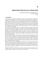
7. Optimization result
In this section, the results obtained using the si mulation are compared with the results ob-
tained using the NN. The criterion function C computed by (15) and the output of NN, C
NN
,
for the vibration control gain K
vc
are plotted in Fig. 16. Comparing the results obtaind using
the NN for the criteri on function with the results obtained using dynamic simulator in Fig. 16.
shows good coincidence. This means that the NN network can successfully replace the dy-
namic simulator to ﬁnd how the criterion function changes with the changing of the system
parameters.
Form Fig. 16 the optimum gain K
vc
can be easily found. One of the main advantages of using
the NN to ﬁnd the optimal gain for the MPID control is the computional speed. To generate
the data of the simulation curve, which is indicated by the triangles in Fig. 16, 1738 seconds is
needed while only 6 seconds are needed to generate the data using the NN, which is indicated

by the circles. The minimum values of the criterion function occur s when the value of the
vibration control gain K
vc
equals 22500 V s/m
2
.
Vibration control gain
Fig. 16. Vibration control gain vs. criterion function.
0 0.5 1 1.5 2 2.5 3 3.5 4 4.5 5
0
6
12
18
24
30
Time [s]
Joint angle [degree]

Optimum Kvc = 17600
PD only Kvc =0
Maximum Kvc = 80000
Fig. 17. Response using optimum gain.
0 0.5 1 1.5 2 2.5 3 3.5 4 4.5 5
0
0.1
0.2
0.3
Time [s]
Tip position [m]

M
t
= 0.5 kg , K
p
= 600, K
d
= 400

Optimum Kvc = 17600
PD only Kvc = 0
Maximum Kvc = 80000
Fig. 18. Response using optimum gain.
Neural Network Based Tuning Algorithm for MPID Control 183
index is also used which is the correlation coefﬁcient r between the two datasets. The correla-
tion coefﬁcient r is 0.9973. When a test is done for the trained NN upon a complete new set of
data the NMSE is 0.0956 and r is 0.9664.
0
Fig. 15. NN training.
7. Optimization result
In this section, the results obtained using the si mulation are compared with the results ob-
tained using the NN. The criterion function C computed by (15) and the output of NN, C
NN
,
for the vibration control gain K
vc
are plotted in Fig. 16. Comparing the results obtaind using
the NN for the criteri on function with the results obtained using dynamic simulator in Fig. 16.
shows good coincidence. This means that the NN network can successfully replace the dy-
namic simulator to ﬁnd how the criterion function changes with the changing of the system

parameters.
Form Fig. 16 the optimum gain K
vc
can be easily found. One of the main advantages of using
the NN to ﬁnd the optimal gain for the MPID control is the computional speed. To generate
the data of the simulation curve, which is indicated by the triangles in Fig. 16, 1738 seconds is
needed while only 6 seconds are needed to generate the data using the NN, which is indicated
by the circles. The minimum values of the criterion function occur s when the value of the
vibration control gain K
vc
equals 22500 V s/m
2
.
Vibration control gain
Fig. 16. Vibration control gain vs. criterion function.
0 0.5 1 1.5 2 2.5 3 3.5 4 4.5 5
0
6
12
18
24
30
Time [s]
Joint angle [degree]

Optimum Kvc = 17600
PD only Kvc =0
Maximum Kvc = 80000
Fig. 17. Response using optimum gain.

0 0.5 1 1.5 2 2.5 3 3.5 4 4.5 5
0
0.1
0.2
0.3
Time [s]
Tip position [m]
M
t
= 0.5 kg , K
p
= 600, K
d
= 400

Optimum Kvc = 17600
PD only Kvc = 0
Maximum Kvc = 80000
Fig. 18. Response using optimum gain.
PID Control, Implementation and Tuning184
0 0.5 1 1.5 2 2.5 3 3.5 4 4.5 5
−0.02
−0.015
−0.01
−0.005
0
0.005
0.01
0.015

0.02
0.025
Time [s]
Deection [m]

Optimum Kvc = 17600
PD only Kvc = 0
Maximum Kvc =80000
Fig. 19. Response using optimum gain.
The resp onse of the ﬂexible manipulator using the optimal gain K
vc
is shown in Fig. 17, Fig. 18
and Fig. 19. 0.5 kg is use d as a tip pay load M
t
with 24 degree for the joint reference angle θ
re f
.
For the controller described by equation (10), the values of K
p
and K
d
are set at 600 V rad/m
and 400 V s rad/m respectively. The response with different vibration gains K
vc
is plotted. In
the beginning the response with PD control only (i.e. K
vc
= 0) is plotted in dash line while
the respo nse with the maximum K

vc
which is 80000 V s/m
2
is plotted i n a dash-dot line. The
response with the optimum K
vc
-which was tuned using NN- appears in a continous line. The
value of the optimum vibration control gain K
vc
is 17600 V s/m
2
. Increasing the vibration
control gain K
vc
leads the system to have fast response for the joint position as shown in
Fig. 17 but more increasing in the value of the vibration control gain leads to an undesirable
overshoot as shown in Fi g. 18 with a dash-dot line. To focus on the effect of the vibration gain
on the end-effector vibration Fig. 19 is plotted. It is clear from the ﬁgure that the optimum
vibration control gain for the MPID succeed to suppress the vibration at the end of the ﬂexible
manipulator.
8. Conclusions
This chapter discusses a NN based gain tuning method for the v ibration control PID (MPID)
controller of a single-link ﬂexible manipulator. The NN is trained to simulate the dynamics
of the single-link ﬂexible manipulator and to produce the integral of the squared tip deﬂec-
tion weighted by exponential function. A dynamic simulator is used to produce the teacher
signals.
The main advantage of using NN to ﬁnd an optimal gain is the computational speed. The NN
based method is approximately 290 times faster than the dynamic simulation based method.
Simulation results with the obtained optimal gain validate the proposed method.
9. References

Cannon, R. H. Jr. & Schmitz, E. (1984). Initial Experiments on the End Point Control of a
Flexible One-Link Robot. International Journal of Robotics Research, Vol. 3, No. 4, pp. 62–
75.
Ge, S. S.; Lee, T. H. & Gong, J. Q. (1999). A Robust Distributed Controller of a Single-Link
SCARA /Cartesian Smart Mater ials Robot, Mechatronics, Vol. 9, No. 1, 1999, pp. 65–
93.
Sun, D.; Shan J.; Su, Y.; Liu H. & Lam, C. (2005). Hybrid Control of a Rotational Fl exible Beam
Using Enhanced PD Feedback with a Non-Linear Differentiator and PZT Actuators,
Smart Mater. Struct., Vol. 14, pp 69–78.
Etxebarria, V.; Sanz, A. & Lizarraga, I. (2005). Control of a Lightweight Flexible Robotic Arm
Using Slid ing Modes, International Journal of Advanced Robotic Systems, Vol. 2, No. 2,
pp. 103–110.
Lee,H. G.; Arimoto, S., & Miyazaki, F. (1988). Liapunov Stability Analysis for PDS Control of
Flexible Multi-link Manipulators, Proceeding of the Conference on Decision and Control,
Austin, pp. 75–80.
Maruyama, T.; Xu, C.; Ming, A. & Shimojo, M. (2006). Motion Control of Ultra-High-Speed
Manipulator with a Flexible Link Based on Dynamically Coupled Driving, Joural of
Robotics and Mechatronics, Vol. 18, No. 5, pp. 598–607.
Matsuno, F. & Hayashi, A. (2000). PDS Cooperative Control of Two One-link Flexible Arms,
Proceeding of the 2000 IEEE International Conference on Robotics and Automation, San
Francisco, pp. 1490–1495.
Talebi, H. A.; Khorasani, K.,& Patel, R. V. (1998).Neural Network Based Control Schemes for
Flexible Link Manipulators: Simulations and Experiments, Neural Networks, Vol. 11,
pp. 1357–1377.
Kawato, M.; Furukawa, K. & Suzuki, R. (1987). A Hierarchical Neural Network Model for
Control and Learning of Voluntary Movement, Biological Cybernetics, Vol. 57, pp. 169–
185.
Isogai, M.; Arai, F. & Fukuda, T. (1999). Intell igent Sensor Fault Detection of Vibration Control
for Flexible Structures, Joural of Robotics and Mechatronics, Vol. 11, No. 6, pp. 524–530.
Lianfang, T.; Wang, J., & Mao, Z. (2004). Constrained Motion Control of Flex ible Robot Ma-

nipulators Based on Recurrent Neural Networks, IEEE Transactions On Systems, Man,
And Cybernetics Part B: Cybernetics, Vol. 34, No. 3, pp. 1541–1552.
Cheng, X . P. & Patel, R. V. (2003). Neural Network Based Tracking Control of a Flexible
Macro
˝
UMicro Manipulator System, Neural Networks, Vol. 16, pp. 271–286.
Yazdizadeh, A.; Khorasani, K. & Patel, R.V. (2000). Identiﬁcation of a Two-Link Flexible Ma-
nipulator Using Adaptive Time Delay Neural Networks, IEEE Transactions On Sys-
tems, Man, And Cybernetics Part B: Cyberneti cs, Vol. 30, No. 1, pp. 165–172.
Ge, S. S.; Lee, T. H. & Zhu, G. ( 1996). Genetic Algorithm Tuning of Lyapunov-Based Con-
trollers" An Application to a Single-Link Flex ible Robot System, IEEE Transactions On
Industrial Electronics, Vol. 43, No. 5, pp. 567–573.
Principe, J.; Euliano, N. & Lefebvre, W. (2000). Neural and Adaptive Systems: Fundamentals
Through Simulations, John Wiley and Sons, New York, pp. 100–172.
Mansour, T.; Konno, A. & Uchiyama, M. (2008). Modiﬁed PID Control of a Single-Link Flexible
Robot, Advanced Robotics, Vol. 22, pp. 433–449.
Neural Network Based Tuning Algorithm for MPID Control 185
0 0.5 1 1.5 2 2.5 3 3.5 4 4.5 5
−0.02
−0.015
−0.01
−0.005
0
0.005
0.01
0.015
0.02
0.025
Time [s]
Deection [m]

Optimum Kvc = 17600
PD only Kvc = 0
Maximum Kvc =80000
Fig. 19. Response using optimum gain.
The resp onse of the ﬂexible manipulator using the optimal gain K
vc
is shown in Fig. 17, Fig. 18
and Fig. 19. 0.5 kg is use d as a tip pay load M
t
with 24 degree for the joint reference angle θ
re f
.
For the controller described by equation (10), the values of K
p
and K
d
are set at 600 V rad/m
and 400 V s rad/m respectively. The response with different vibration gains K
vc
is plotted. In
the beginning the response with PD control only (i.e. K
vc
= 0) is plotted in dash line while
the respo nse with the maximum K
vc
which is 80000 V s/m
2
is plotted i n a dash-dot line. The

response with the optimum K
vc
-which was tuned using NN- appears in a continous line. The
value of the optimum vibration control gain K
vc
is 17600 V s/m
2
. Increasing the vibration
control gain K
vc
leads the system to have fast response for the joint position as shown in
Fig. 17 but more increasing in the value of the vibration control gain leads to an undesirable
overshoot as shown in Fi g. 18 with a dash-dot line. To focus on the effect of the vibration gain
on the end-effector vibration Fig. 19 is plotted. It is clear from the ﬁgure that the optimum
vibration control gain for the MPID succeed to suppress the vibration at the end of the ﬂexible
manipulator.
8. Conclusions
This chapter discusses a NN based gain tuning method for the v ibration control PID (MPID)
controller of a single-link ﬂexible manipulator. The NN is trained to simulate the dynamics
of the single-link ﬂexible manipulator and to produce the integral of the squared tip deﬂec-
tion weighted by exponential function. A dynamic simulator is used to produce the teacher
signals.
The main advantage of using NN to ﬁnd an optimal gain is the computational speed. The NN
based method is approximately 290 times faster than the dynamic simulation based method.
Simulation results with the obtained optimal gain validate the proposed method.
9. References
Cannon, R. H. Jr. & Schmitz, E. (1984). Initial Experiments on the End Point Control of a
Flexible One-Link Robot. International Journal of Robotics Research, Vol. 3, No. 4, pp. 62–
75.
Ge, S. S.; Lee, T. H. & Gong, J. Q. (1999). A Robust Distributed Controller of a Single-Link

SCARA /Cartesian Smart Mater ials Robot, Mechatronics, Vol. 9, No. 1, 1999, pp. 65–
93.
Sun, D.; Shan J.; Su, Y.; Liu H. & Lam, C. (2005). Hybrid Control of a Rotational Fl exible Beam
Using Enhanced PD Feedback with a Non-Linear Differentiator and PZT Actuators,
Smart Mater. Struct., Vol. 14, pp 69–78.
Etxebarria, V.; Sanz, A. & Lizarraga, I. (2005). Control of a Lightweight Flexible Robotic Arm
Using Slid ing Modes, International Journal of Advanced Robotic S ystems, Vol. 2, No. 2,
pp. 103–110.
Lee,H. G.; Arimoto, S., & Miyazaki, F. (1988). Liapunov Stability Analysis for PDS Control of
Flexible Multi-link Manipulators, Proceeding of the Conference on Decision and Control,
Austin, pp. 75–80.
Maruyama, T.; Xu, C.; Ming, A. & Shimojo, M. (2006). Motion Control of Ultra-High-Speed
Manipulator with a Flexible Link Based on Dynamically Coupled Driving, Joural of
Robotics and Mechatronics, Vol. 18, No. 5, pp. 598–607.
Matsuno, F. & Hayashi, A. (2000). PDS Cooperative Control of Two One-link Flexible Arms,
Proceeding of the 2000 IEEE International Conference on Robotics and Automation, San
Francisco, pp. 1490–1495.
Talebi, H. A.; Khorasani, K.,& Patel, R. V. (1998).Neural Network Based Control Schemes for
Flexible Link Manipulators: Simulations and Experiments, Neural Networks, Vol. 11,
pp. 1357–1377.
Kawato, M.; Furukawa, K. & Suzuki, R. (1987). A Hierarchical Neural Network Model for
Control and Learning of Voluntary Movement, Biological Cybernetics, Vol. 57, pp. 169–
185.
Isogai, M.; Arai, F. & Fukuda, T. (1999). Intelligent Senso r Fault Detection of Vibration Control
for Flexible Structures, Joural of Robotics and Mechatronics, Vol. 11, No. 6, pp. 524–530.
Lianfang, T.; Wang, J., & Mao, Z. (2004). Constrained Motion Control of Flex ible Robot Ma-
nipulators Based on Recurrent Neural Networks, IEEE Transactions On Systems, Man,
And Cybernetics Part B: Cybernetics, Vol. 34, No. 3, pp. 1541–1552.
Cheng, X . P. & Patel, R. V. (2003). Neural Network Based Tracking Control of a Flexible
Macro

˝
UMicro Manipulator System, Neural Networks, Vol. 16, pp. 271–286.
Yazdizadeh, A.; Khorasani, K. & Patel, R.V. (2000). Identiﬁcation of a Two-Link Flexible Ma-
nipulator Using Adaptive Time Delay Neural Networks, IEEE Transactions On Sys-
tems, Man, And Cybernetics Part B: Cyberneti cs, Vol. 30, No. 1, pp. 165–172.
Ge, S. S.; Lee, T. H. & Zhu, G. ( 1996). Genetic Algorithm Tuning of Lyapunov-Based Con-
trollers" An Application to a Single-Link Flex ible Robot System, IEEE Transactions On
Industrial Electronics, Vol. 43, No. 5, pp. 567–573.
Principe, J.; Euliano, N. & Lefebvre, W. (2000). Neural and Adaptive Systems: Fundamentals
Through Simulations, John Wiley and Sons, New York, pp. 100–172.
Mansour, T.; Konno, A. & Uchiyama, M. (2008). Modiﬁed PID Control of a Single-Link Flexible
Robot, Advanced Robotics, Vol. 22, pp. 433–449.

Adaptive PID Control for Asymptotic Tracking Problem of MIMO Systems 187
Adaptive PID Control for Asymptotic Tracking Problem of MIMO Systems
Kenichi Tamura and Hiromitsu Ohmori
0
Adaptive PID Control for Asymptotic Tracking
Problem of MIMO Systems
Kenichi Tamura
1
and Hiromitsu Ohmori
2
1
Tokyo Metropolitan University
2
Keio University
JAPAN
1. Introduction
PID control, which is usually known as a classical output feedback control for SISO systems,

has been widely used in the industrial world(Åström & Hägglund, 1995; Suda, 1992). The
tuning methods of PID control are adjusting the proportional, the integral and the derivative
gains to make an output of a controlled system track a target value properly. There exist much
more researches on tuning methods of PID control for SISO systems than MIMO systems
although more MIMO systems actually exist than SISO systems. The tuning methods for SISO
systems are difﬁcult to apply to PID control for MIMO systems since the gains usually become
matrices in such case.
MIMO systems usually tend to have more complexities and uncertainties than SISO systems.
Several tuning methods of PID control for such MIMO system are investigated as follows.
From off-line approach, there are progressed classical loop shaping based methods (Ho
et al., 2000; Hara et al., 2006) and H
∞
control theory based methods (Mattei, 2001; Saeki,
2006; Zheng et al., 2002). From on-line approach, there are methods from self-tuning control
such as the generalized predictive control based method (Gomma, 2004), the generalized
minimum variance control based method (Yusof et al., 1994), the model matching based
method (Yamamoto et al., 1992) and the method using neural network (Chang et al., 2003).
These conventional methods often require that the MIMO system is stable and are usually
used for a regulator problem for a constant target value but a tracking problem for
a time-varying target value, which restrictions narrow their application. So trying these
problems is signiﬁcant from a scientiﬁc standpoint how there is possibility of PID control and
from a practical standpoint of expanding applications. In MIMO case, there is possibility to
solve these problems because PID control has more freedoms in tuning of PID gain matrices.
On the other hand, adaptive servo control is known for a problem of the asymptotic output
tracking and/or disturbances rejection to unknown systems under guaranteeing stability.
There are researches for SISO systems (Hu & Tomizuka, 1993; Miyasato, 1998; Ortega & Kelly,
1985) and for MIMO systems (Chang & Davison, 1995; Dang & Owens, 2006; Johansson, 1987).
Their controllers generally depend on structures of the controlled system and the reference
system, which features are undesirable from standpoint of utility (Saeki, 2006; Miyamoto,
1999). So it is important to develop the ﬁxed controller like PID controller to solve the servo

problem and to show that conditions. But they are difﬁcult to apply to the tuning of PID
controller because of differences of their construction.
In this paper, we consider adaptive PID control for the asymptotic output tracking problem of
MIMO systems with unknown system parameters under existence of unknown disturbances.
9
PID Control, Implementation and Tuning188
The proposed PID controller has constant gain matrices and adjustable gain matrices. The
proposed adaptive tuning laws of the gain matrices are derived by using Lyapunov theorem.
That is a Lyapunov function based on characteristics of the proposed PID controller is
constructed. This method guarantees the asymptotic output tracking even if the controlled
MIMO system is unstable and has uncertainties and unknown constant disturbances. Finally,
the effectiveness of the proposed method is conﬁrmed with simulation results for the 8-state,
2-input and 2-output missile control system and the 4-state, 2-input and 2-output unstable
system.
2. Problem statement
Consider the MIMO system:
˙
x
(t) = Ax(t) + Bu(t) + d
i
, (1)
y
(t) = Cx(t) + d
o
, (2)
where x
(t) ∈ R
n
, u(t) ∈ R
m

, y(t) ∈ R
m
are the state vector, the input vector and the output
vector respectively, d
i
∈ R
n
, d
o
∈ R
m
are unknown constant disturbances, and A, B, C are
unknown system matrices.
The target signal of the output is y
M
(t) ∈ R
m
generated by the reference system:
˙
x
M
(t) = A
M
x
M
(t) + B
M
u
M
, (3)

y
M
(t) = C
M
x
M
(t), (4)
where x
M
(t) ∈ R
n
M
and u
M
∈ R
r
M
are the state vector and the constant input vector,
respectively. Note that A
M
, B
M
, C
M
are allowed to be unknown matrices.
In this article, we propose the new adaptive PID controller:
u
(t) = K
I0


t
0
e
y
(τ)dτ + (K
P0
+ K
P1
(t))e
y
(t) + K
D1
(t)
˙
e
y
(t) + K
P2
(t)y
M
(t) + K
D2
(t)
˙
y
M
(t) (5)
which has the adjustable gain matrices K
P1
(t), K

P2
(t), K
D1
(t), K
D2
(t) ∈ R
m×m
and the
constant gain matrices K
I0
, K
P0
∈ R
m×m
, and
e
y
(t) = y
M
(t) − y(t) (6)
denotes the error of the output from the target signal y
M
(t). The diagram of the proposed PID
controller is shown in Fig. 1.
The objective is to design the constant gain matrices K
I0
, K
P0
and the adaptive tuning laws
of the adjustable gain matrices K

P1
(t), K
P2
(t), K
D1
(t), K
D2
(t) to solve the asymptotic output
tracking, i.e. e
y
(t) → 0 as t → ∞.
Here we assume the following conditions:
Assumption 1: rank

A B
C 0

= n + m, and λ
i
(M
11
)λ
j
(A
M
) = 1,i = 1, 2, · · · , n, j = 1,2, · · · , n
M
,
where


M
11
M
12
M
21
M
22

:
=

A B
C 0

−1
, M
11
∈ R
n×n
and λ(·) denotes eigenvalues of a matrix.
Assumption 2: rank

C
M
C
M
A
M


= n
M
.
Assumption 3: The zero-dynamics of
{A, B, C} is asymptotically stable.
Assumption 4: (a) CB
= 0, CAB > 0 or (b) CB > 0.
Let us explain these assumptions. Assumption 1 is well known condition for a servo problem.
Assumption 2 means the output of the reference system and its derivative contain the
information of its state. Assumption 3 equals to the minimum phase property of the controlled
system. Assumption 4 contains the condition that the relative degrees are
≤ 2. It is inevitable
that these conditions seem a little severe because these are conditions for the PID controller
that has the structural constraint. But also there is an advantage that the controlled system’s
stability property, which is often assumed in other PID control’s methods, is not assumed.
Fig. 1. Proposed Adaptive PID Controller
3. Error system with proposed adaptive PID controller
In this section, we derive the error system with the adaptive PID controller. When the perfect
output tracking occurs (i.e. y
(t) = y
M
(t), ∀t ≥ 0), we can deﬁne the corresponding state and
input trajectories as x
∗
(t), u
∗
(t), respectively. That is x
∗
(t), u
∗

(t) are trajectories satisfying the
following relation:
˙
x
∗
(t) = Ax
∗
(t) + Bu
∗
(t) + d
i
, (7)
y
M
(t) = Cx
∗
(t) + d
o
, ∀t ≥ 0. (8)
From Appendix A inspired by (Kaufman et al., 1994), there exist matrices M
ij
, T
ij
, i, j = 1,2
under Assumption 1, and the ideal trajectories x
∗
(t), u
∗
(t) satisfying relations (7), (8) can be
expressed as

x
∗
(t) = T
11
x
M
(t) + T
12
u
M
− M
11
d
i
− M
12
d
o
, (9)
u
∗
(t) = T
21
x
M
(t) + T
22
u
M
− M

21
d
i
− M
22
d
o
. (10)
Introducing these ideal trajectories, we can deﬁne the following state error
e
x
(t) = x
∗
(t) − x(t). (11)
Then, the output tracking error (6) can be described as
e
y
(t) = y
M
(t) − y(t) = (Cx
∗
(t) + d
o
) − (Cx(t) + d
o
) = Ce
x
(t), (12)
which means that if the error system obtained by differentiating (11):
˙

e
x
(t) = Ae
x
(t) + B( u
∗
(t) − u(t)) (13)
can be asymptotically stabilized i.e. e
x
(t) → 0, then the asymptotic output tracking can be
achieved i.e. e
y
(t) → 0.
Now, substituting (5) and (10) into (13), we get the following closed loop error system:
˙
e
x
(t) = Ae
x
(t) − B

− T
21
x
M
(t) − T
22
u
M
+ M

21
d
i
+ M
22
d
o
+ K
I0

t
0
e
y
(τ)dτ
+ K
P0
e
y
(t) + K
P1
(t)e
y
(t) + K
D1
(t)
˙
e
y
(t) + K

P2
(t)y
M
(t) + K
D2
(t)
˙
y
M
(t)

. (14)
Adaptive PID Control for Asymptotic Tracking Problem of MIMO Systems 189
The proposed PID controller has constant gain matrices and adjustable gain matrices. The
proposed adaptive tuning laws of the gain matrices are derived by using Lyapunov theorem.
That is a Lyapunov function based on characteristics of the proposed PID controller is
constructed. This method guarantees the asymptotic output tracking even if the controlled
MIMO system is unstable and has uncertainties and unknown constant disturbances. Finally,
the effectiveness of the proposed method is conﬁrmed with simulation results for the 8-state,
2-input and 2-output missile control system and the 4-state, 2-input and 2-output unstable
system.
2. Problem statement
Consider the MIMO system:
˙
x
(t) = Ax(t) + Bu(t) + d
i
, (1)
y
(t) = Cx(t) + d

o
, (2)
where x
(t) ∈ R
n
, u(t) ∈ R
m
, y(t) ∈ R
m
are the state vector, the input vector and the output
vector respectively, d
i
∈ R
n
, d
o
∈ R
m
are unknown constant disturbances, and A, B, C are
unknown system matrices.
The target signal of the output is y
M
(t) ∈ R
m
generated by the reference system:
˙
x
M
(t) = A
M

x
M
(t) + B
M
u
M
, (3)
y
M
(t) = C
M
x
M
(t), (4)
where x
M
(t) ∈ R
n
M
and u
M
∈ R
r
M
are the state vector and the constant input vector,
respectively. Note that A
M
, B
M
, C

M
are allowed to be unknown matrices.
In this article, we propose the new adaptive PID controller:
u
(t) = K
I0

t
0
e
y
(τ)dτ + (K
P0
+ K
P1
(t))e
y
(t) + K
D1
(t)
˙
e
y
(t) + K
P2
(t)y
M
(t) + K
D2
(t)

˙
y
M
(t) (5)
which has the adjustable gain matrices K
P1
(t), K
P2
(t), K
D1
(t), K
D2
(t) ∈ R
m×m
and the
constant gain matrices K
I0
, K
P0
∈ R
m×m
, and
e
y
(t) = y
M
(t) − y(t) (6)
denotes the error of the output from the target signal y
M
(t). The diagram of the proposed PID

controller is shown in Fig. 1.
The objective is to design the constant gain matrices K
I0
, K
P0
and the adaptive tuning laws
of the adjustable gain matrices K
P1
(t), K
P2
(t), K
D1
(t), K
D2
(t) to solve the asymptotic output
tracking, i.e. e
y
(t) → 0 as t → ∞.
Here we assume the following conditions:
Assumption 1: rank

A B
C 0

= n + m, and λ
i
(M
11
)λ
j

(A
M
) = 1,i = 1, 2, · · · , n, j = 1,2, · · · , n
M
,
where

M
11
M
12
M
21
M
22

:
=

A B
C 0

−1
, M
11
∈ R
n×n
and λ(·) denotes eigenvalues of a matrix.
Assumption 2: rank


C
M
C
M
A
M

= n
M
.
Assumption 3: The zero-dynamics of
{A, B, C} is asymptotically stable.
Assumption 4: (a) CB
= 0, CAB > 0 or (b) CB > 0.
Let us explain these assumptions. Assumption 1 is well known condition for a servo problem.
Assumption 2 means the output of the reference system and its derivative contain the
information of its state. Assumption 3 equals to the minimum phase property of the controlled
system. Assumption 4 contains the condition that the relative degrees are
≤ 2. It is inevitable
that these conditions seem a little severe because these are conditions for the PID controller
that has the structural constraint. But also there is an advantage that the controlled system’s
stability property, which is often assumed in other PID control’s methods, is not assumed.
Fig. 1. Proposed Adaptive PID Controller
3. Error system with proposed adaptive PID controller
In this section, we derive the error system with the adaptive PID controller. When the perfect
output tracking occurs (i.e. y
(t) = y
M
(t), ∀t ≥ 0), we can deﬁne the corresponding state and
input trajectories as x

∗
(t), u
∗
(t), respectively. That is x
∗
(t), u
∗
(t) are trajectories satisfying the
following relation:
˙
x
∗
(t) = Ax
∗
(t) + Bu
∗
(t) + d
i
, (7)
y
M
(t) = Cx
∗
(t) + d
o
, ∀t ≥ 0. (8)
From Appendix A inspired by (Kaufman et al., 1994), there exist matrices M
ij
, T
ij

, i, j = 1,2
under Assumption 1, and the ideal trajectories x
∗
(t), u
∗
(t) satisfying relations (7), (8) can be
expressed as
x
∗
(t) = T
11
x
M
(t) + T
12
u
M
− M
11
d
i
− M
12
d
o
, (9)
u
∗
(t) = T
21

x
M
(t) + T
22
u
M
− M
21
d
i
− M
22
d
o
. (10)
Introducing these ideal trajectories, we can deﬁne the following state error
e
x
(t) = x
∗
(t) − x(t). (11)
Then, the output tracking error (6) can be described as
e
y
(t) = y
M
(t) − y(t) = (Cx
∗
(t) + d
o

) − (Cx(t) + d
o
) = Ce
x
(t), (12)
which means that if the error system obtained by differentiating (11):
˙
e
x
(t) = Ae
x
(t) + B( u
∗
(t) − u(t)) (13)
can be asymptotically stabilized i.e. e
x
(t) → 0, then the asymptotic output tracking can be
achieved i.e. e
y
(t) → 0.
Now, substituting (5) and (10) into (13), we get the following closed loop error system:
˙
e
x
(t) = Ae
x
(t) − B

− T
21

x
M
(t) − T
22
u
M
+ M
21
d
i
+ M
22
d
o
+ K
I0

t
0
e
y
(τ)dτ
+ K
P0
e
y
(t) + K
P1
(t)e
y

(t) + K
D1
(t)
˙
e
y
(t) + K
P2
(t)y
M
(t) + K
D2
(t)
˙
y
M
(t)

. (14)
PID Control, Implementation and Tuning190
From Appendix B, there exist matrices S
1
, S
2
∈ R
m×m
under Assumption 2, and T
21
x
M

(t) in
(14) can be decomposed as
T
21
x
M
(t) = S
1
y
M
(t) + S
2
(
˙
y
M
(t) − C
M
B
M
u
M
). (15)
Hence, (14) can be expressed as
˙
e
x
(t) = Ae
x
(t) − B


(S
2
C
M
B
M
− T
22
)u
M
+ M
21
d
i
+ M
22
d
o
+ K
I0

t
0
e
y
(τ)dτ + K
P0
e
y

(t)
+
K
P1
(t)e
y
(t) + K
D1
(t)
˙
e
y
(t) + (K
P2
(t) − S
1
)y
M
(t) + (K
D2
(t) − S
2
)
˙
y
M
(t)

. (16)
Here put the constant term of the above equation as


d :
= (S
2
C
M
B
M
− T
22
)u
M
+ M
21
d
i
+ M
22
d
o
to represent (16) simply as
˙
e
x
(t) = Ae
x
(t) − B


d + K

I0

t
0
e
y
(τ)dτ + K
P0
e
y
(t) + K
P1
(t)e
y
(t) + K
D1
(t)
˙
e
y
(t)
+ (
K
P2
(t) − S
1
)y
M
(t) + (K
D2

(t) − S
2
)
˙
y
M
(t)

. (17)
Therefore, if the origin of this close-loop error system is asymptotically stabilized i.e. e
x
(t) →
0, the asymptotic output tracking i.e. e
y
(t) → 0 is achieved. We derive the constant gain
matrices and the adaptive tuning laws of adjustable gain matrices to accomplish e
x
(t) → 0
in the next section.
4. Adaptive tuning laws of PID gain matrices
In this section, we show the constant gain matrices K
I0
, K
P0
and the adaptive tuning law of
the adjustable gain matrices K
P1
(t), K
P2
(t), K

D1
(t), K
D2
(t) to asymptotically stabilize the error
dynamics (17) (i.e. e
x
→ 0 as t → ∞) at Case A when Assumption 4(a) is hold or at Case B when
Assumption 4(b) is hold.
4.1 Case A
Theorem 1: Suppose Assumption 3 and Assumption 4(a). Give the constant gain matrices
K
I0
, K
P0
as
K
I0
= γ
I
H
1
, K
P0
= γ
I
H
2
, (18)
and the adaptive tuning laws of the adjustable gain matrices K
Pi

(t), K
Di
(t), i = 1, 2 as
˙
K
P1
(t) = Γ
P1

H
1
e
y
(t) + H
2
˙
e
y
(t)

e
y
(t)
T
, (19a)
˙
K
D1
(t) = Γ
D1


H
1
e
y
(t) + H
2
˙
e
y
(t)

˙
e
y
(t)
T
, (19b)
˙
K
P2
(t) = Γ
P2

H
1
e
y
(t) + H
2

˙
e
y
(t)

y
M
(t)
T
, (19c)
˙
K
D2
(t) = Γ
D2

H
1
e
y
(t) + H
2
˙
e
y
(t)

˙
y
M

(t)
T
(19d)
where
H
1
= diag{h
11
, · · · , h
1m
}, H
2
= diag{h
21
, · · · , h
2m
}, h
1j
, h
2j
> 0, j = 1, · · · , m, (20)
then the origin of (17) is asymptotically stable (e
x
(t) → 0 as t → ∞) and the adjustable gain
matrices are bounded. Here Γ
P1
, Γ
P2
, Γ
D1

, Γ
D2
∈ R
m×m
are arbitrary positive deﬁnite matrices
and γ
I
is arbitrary positive scalar.
Proof: From Assumption 4(a), the error dynamics (17) is transformed into the normal form
(see e.g. (Isidori, 1995)):


˙
ξ
1
(t)
˙
ξ
2
(t)
˙
η
(t)


=


0 I
m

0
Q
21
Q
22
Q
23
Q
31
Q
32
A
η




ξ
1
(t)
ξ
2
(t)
η(t)


−


0

CAB
0



K
I0

t
0
ξ
1
(τ)dτ + K
P0
ξ
1
(t) +

d
+ K
P1
(t)ξ
1
(t) + K
D1
(t)ξ
2
(t) + (K
P2
(t) − S

1
)y
M
(t) + (K
D2
(t) − S
2
)
˙
y
M
(t)

, (21)
which Q
ij
are unknown matrices, by transformation


ξ
1
(t)
ξ
2
(t)
η(t)


=



C
CA
T


e
x
(t) (22)
where TB
= 0, T ∈ R
(n−2m)×n
and
ξ
1
(t) = Ce
x
(t) = e
y
(t), ξ
2
(t) = CAe
x
(t) =
˙
e
y
(t). (23)
Note that when ξ
1

(t), ξ
2
(t) ≡ 0,
˙
η
(t) = A
η
η(t), (24)
which is called zero-dynamics, is asymptotic stable from Assumption 3.
Thus (21) is can be rewritten as


˙
ξ
1
(t)
˙
ξ
2
(t)
˙
η
(t)


=


0 I
m

0
−K
ξ1
−K
ξ2
Q
23
Q
31
Q
32
A
η




ξ
1
(t)
ξ
2
(t)
η(t)


−


0

I
m
0



CAB
(K
I0

t
0
ξ
1
(τ)dτ + K
P0
ξ
1
(t) +

d
)
+ (
CABK
P1
(t) − Q
21
− K
ξ1
)ξ

1
(t) + (CABK
D1
(t) − Q
22
− K
ξ2
)ξ
2
(t)
+
CAB(K
P2
(t) − S
1
)y
M
(t) + CAB(K
D2
(t) − S
2
)
˙
y
M
(t)

(25)
where K
ξ1

, K
ξ2
∈ R
m×m
are the constant matrices only used in the proof.
For simplicity, put
ξ
(t) :=

ξ
1
(t)
ξ
2
(t)

, A
ξ
:=

0 I
m
0 0

, B
ξ
:=

0
I

m

, (26)
K
ξ
:=

K
ξ1
K
ξ2

, Q
1
:=

0
Q
23

, Q
2
:=
[
Q
31
Q
32
]
, (27)

ψ
I
(t) := CAB(K
I0

t
0
ξ
1
(τ)dτ + K
P0
ξ
1
(t) +

d
), (28)
Ψ
P1
(t) := CABK
P1
(t) − Q
21
− K
ξ1
, (29a)
Ψ
D1
(t) := CABK
D1

(t) − Q
22
− K
ξ2
, (29b)
Ψ
P2
(t) := CAB(K
P2
(t) − S
1
), (29c)
Ψ
D2
(t) := CAB(K
D2
(t) − S
2
) (29d)
Adaptive PID Control for Asymptotic Tracking Problem of MIMO Systems 191
From Appendix B, there exist matrices S
1
, S
2
∈ R
m×m
under Assumption 2, and T
21
x
M