Sliding Mode Control Part 11 pptx
Bạn đang xem bản rút gọn của tài liệu. Xem và tải ngay bản đầy đủ của tài liệu tại đây (1.7 MB, 35 trang )
High Order Sliding Mode Control for Suppression of
Nonlinear Dynamics in Mechanical Systems with Friction
339
• Although a rigorous robustness analysis is beyond the scope of this study, numerical
examples will show that the feedback controller is able of yielding robust control
performance despite significant parameter departures from parameter nominal values.
• Stability must be preserved in the context of both structured uncertainties in the
parameters as well as unstructured errors in modeling. A stability analysis for the
proposed control configurations should parallel the steps reported in (Aguilar-Lopez et
al., 2010) and (Aguilar-López & Martínez-Guerra, 2008).
4. Applications
In this section, simulation results are presented for both position regulation and tracking
of mechanical systems with friction (7) with the IHOSMC approach described above. The
control performance is evaluated considering set point changes and typical disturbances of
mechanical systems. We consider the following five examples: (i) Mechanical system with
Coulomb friction, (ii) an inverted pendulum, (iii) an AC induction motor, and (vi) a levitation
magnetic system.
4.1 Mechanical system with Coulomb friction
We consider a mechanical system described in (Alvarez-Ramirez et al., 1995) with a Coulomb
friction law. The dimensionless equation of motion is,
dx1
= x2
dt
1
dx2
=
{− F ( x1, x2 ) − αx1 + τl + u }
dt
m
(18)
where m is the mass of the system, τl is an unknown external force, which way be due to
loads and/or noise acting in the mechanism, u is a manipulated forced used to control the
system and the term F ( x1 , x2 ) includes all friction effects and is determined by the following
expression,
F ( x1, x2 ) = φ f ( x1 )
where φ is the coefficient of friction and f ( x1 ) is the normal load which vary with
displacement,
f ( x1 ) = − μ k x1 < 0
(19)
− μ s ≤ f ( x1 ) ≤ μ s x1 = 0
f ( x1 ) = μ k x1 > 0
Control objetive is the position tracking to the periodic reference,
yre f = x1,re f = 0.3 sin(0.5t)
The parameters of the controller are set as δ1,i = [25, 10], and δ2,i = [2.3, 1]. Model simulation
parameters are taken from (Alvarez-Ramirez et al., 1995). The control law is turned on the
t = 50 time units and τl = A sin(1.25t). At t = 75 the amplitude A of the external force τl is
340
Sliding Mode Control
2
10
(a)
(b)
8
1.5
Control input, u
6
Position, x
1
1
0.5
0
4
2
0
−2
−4
−0.5
−6
−1
−8
−1.5
0
10
20
30
40
50
Time
60
70
80
90
100
0
10
20
30
40
50
Time
60
70
80
90
100
Fig. 2. (a) Cascade control for mechanical system, (18) and (b) control input.
changed in 20 %. Figure 2 shows the position trajectory before and after the control activation.
In Figure 2 the control input is also displayed. It can be seen that the proposed cascade control
scheme is able to track the desired reference and rejects the applied perturbation. After that
the control input reach the saturation levels (−10 < u < 10) the control inputs displays a
complex oscillatory behavior.
4.2 Inverted pendulum
The inverted pendulum has been used as a classical control example for nearly half a century
because of its nonlinear, unstable, and nonminimum-phase characteristics. In this case we
consider a single inverted pendulum.
The equation of motion for a simple inverted pendulum with Coulomb friction and external
perturbation is (Poznyak et al., 2006),
dx1
= x2
dt
dx2
= − g sin( x1 )/l − vs x2 /J − ps sign ( x2 )/J + τd + u/J
dt
(20)
where g is the gravitational acceleration, l is the distance between the rotational axis and
center of gravity of the pendulum, J = ml 2 is the inertial moment, where m is the mass of the
system, τd = 0.5 sin(2t) + 0.5 cos(5t) is an external disturbance, which may be due to loads
and/or noise acting in the mechanism, u is a manipulated forced used to control the system.
Let yre f = x1,re f = sin(t) be the desired orbit of the pendulum position. Figure 3 shows the
control performance using the control parameters δ1,i = [12, 7], and δ2,i = [1, 0.5]. In this case
the IHOSMC controller is activated at t = 15 and from 0 to 15 time units the pendulum is
driven by the twisting controller introduced by Poznyak et al. (2006). It can be seen from
Figure 3 that the IHOSMC controller is able to follow the periodic orbit with a better closed
loop behavior that the twisting controller.
High Order Sliding Mode Control for Suppression of
Nonlinear Dynamics in Mechanical Systems with Friction
1.5
50
(a)
(b)
40
30
Control input, u
1
Position, x1
341
0.5
0
20
10
0
−10
−20
−0.5
−30
−40
−1
0
5
10
15
20
25
30
−50
0
5
Time
10
15
20
25
30
Time
Fig. 3. (a) Control performance for inverted pendulum system and (b) control input.
4.3 Induction AC motors
Induction motors have found considerable applications in industry due to their reliability,
ruggedness and relatively low cost. Their mechanical reliability is due to the fact that there
is no mechanical commutation as in most DC motors. Furthermore, induction motors can
also be used in volatile environments because no sparks are produced. An induction motor is
composed of three stator windings and three rotor windings.
A simple mathematical model of an induction motor, under field-oriented control with a
constant rotor flux amplitude, which was presented in (Tan et al., 2003), is the following,
dx1
= x2
dt
K
F
τ
dx2
= T x3 − − l
dt
J
J
J
dx3
= a1 x2 + a2 x3 + bu
dt
(21)
where x1 is the rotor angle, x2 is the rotor angular velocity, x3 is the component of stator
current, u is the component of stator voltage, J is the rotor inertia, τl is the load torque, and F
is the friction force.
Friction force is modeled by the LuGre friction model with friction force variations,
dz
| x2 |
= x2 −
z
dt
g ( x2 )
dz
F = σ0 z + σ1
+ σ2 x2
dt
(22)
342
Sliding Mode Control
6
15
(a)
10
Control input, u
Rotor angle, x1
4
(b)
2
0
5
0
−2
−5
−4
−10
−6
0
50
100
150
200
250
300
−15
0
50
Time
100
150
200
250
300
Time
Fig. 4. (a) Cascade control for induction AC motors system and (b) control input.
where z is the friction state that physically stands for the average deflection of the bristles
between two contact surfaces. The nonlinear function is used to describe different friction
effects and can be parameterized to characterize the Stribeck effect,
x2 2
)
(23)
vs
where Fc is the Coulomb friction value, Fs is the stiction force value, and vs is the Stribeck
velocity.
The control objective is to asymptotically track a given bounded reference signal yre f = x1,re f
given by,
g( x2 ) = Fc + ( Fs − Fc ) exp(−
yre f = 5.6 sin(0.4πt) sin(0.02πt)
(24)
A load disturbance τl = 0.8 N · m is injected into the induction motor simulation model. The
position of the rotor angle and the corresponding control input are shown in Figure 4. It can be
seen that the controller is able to track the desired reference (24) using a periodic input of the
control input. The external disturbance is also rejected without an appreciable degradation of
the closed-loop system.
4.4 Levitation system
Magnetic levitation systems have been receiving considerable interest due to their great
practical importance in many engineering fields (Hikihara & Moon, 1994). For instance,
high-speed trains, magnetic bearings, coil gun and high-precision platforms. We consider
the control of the vertical motion in a class of magnetic levitation given by a single degree
of freedom (specifically, a magnet supported by a superconducting system). In particular,
we consider a magnet supported by superconducting system which can be represented by
a second-order differential equation with a nonlinear term which involves hysteresis and
periodic external excitation force. Without loss of generality, one can consider that the model
of the levitation system is modelled by the following equation (Femat, 1998),
High Order Sliding Mode Control for Suppression of
Nonlinear Dynamics in Mechanical Systems with Friction
dx1
= x2
dt
dx2
= − δx2 − x1 + x3 + τl + u
dt
dx3
= − γ ( x3 − F )
dt
343
(25)
x1 is defined as a displacement from the surface of a high Tc superconductor (HTSC) surface,
x2 is the velocity, x3 is a dynamical force between the HTSC and the magnet, which includes
hysteresis effects, δ represents a mechanical damping coefficient, γ is a relaxation coefficient,
τl is an external excitation force, and u is the control force.
The nonlinear function F is given by (Femat, 1998),
F = Fx1 exp(− x1 )(1 − Fx2 )
(26)
Fx1 = F0 exp(− x1 )
⎧
⎪ − μ 1 − x2
≤ x2
⎨
− x2 ( μ1 − μ2 )
Fx1 =
− ≤ x2 <
2
⎪
⎩
μ2
x2 < −
where the exponential term Fx1 shows the force-displacement relation without hysteresis, F0
denotes the maximum force between the HTSC and the magnet, μ1 and μ2 are constants. The
control problem is the regulation to the origin of the vertical motion, i.e. yre f = x1,re f = 0.0. In
the Figure 6 the controlled position and the corresponding control input are presented (control
action is turn on a t = 100.0 time units). It can be seen from Figure 5 that the controller can
regulate the vertical position of the levitation system via a simple periodic manipulation of
the control force. The control input reaches saturation levels in the first 20 time units, which
can be related to high values of the controller parameters.
5. Conclusions
In mechanical systems, the control performance is greatly affected by the presence of several
significant nonlinearities such as static and dynamic friction, backlash and actuator saturation.
Hence, the productivity of industrial systems based on mechanical systems depend upon how
control approaches are able to compensate these adverse effects. Indeed, fiction in mechanical
systems can lead to premature degradation of highly expensive mechanical and electronic
components. On the other hand, due to uncertainties and variations in environmental factors
a mathematical model of the friction phenomena present significant uncertainties.
In this chapter, by means of an IHOSMC approach and a cascade control configuration
we have derived a robust control approach for both regulation and tracking position in
mechanical systems. The underlying idea behind the control approach is to force the error
dynamics to a sliding surface that compensates uncertain parameters and unknown term.
The sliding mode control law is enhanced with an uncertainties observer. We have show via
numerical simulations how the motion can be regulate and tracking to a desired reference in
presence of uncertainties in the control design and changes in model parameters. Although
344
Sliding Mode Control
1.2
0.5
(a)
1
0.3
0.6
0.2
Control input, u
0.8
Position, x1
(b)
0.4
0.4
0.2
0.1
0
0
−0.1
−0.2
−0.2
−0.4
−0.3
−0.6
−0.4
−0.5
−0.8
0
20
40
60
80
100 120 140 160 180 200
Time
0
20
40
60
80
100 120 140 160 180 200
Time
Fig. 5. Levitation system: (a) motion vertical control and (b) control input.
the control design is restricted to certain class of mechanical systems with friction, the concepts
presented in our work should find general applicability in the control of friction in other
systems.
6. References
Aguilar-Lopez, R.; Martinez-Guerra, R.; Puebla, H. & Hernadez-Suarez, R. (2010). High order
sliding-mode dynamic control for chaotic intracellular calcium oscillations. Nonlinear
Analysis B: Real World Applications, 11, 217-231.
Aguilar-Lopez, R. & Martinez-Guerra, R. (2008). Control of chaotic oscillators via a class of
model free active controller: suppression and synchronization. Chaos Solitons Fractals,
38, No. 2, 531-540.
Alvarez-Ramirez, J. (1999). Adaptive control of feedback linearizable systems: a modelling
error compensation approach. Int. J. Robust Nonlinear Control, 9, 361.
Alvarez-Ramirez, J.; Alvarez, J. & Morales, A. (2002). An adaptive cascade control for a class
of chemical reactors, International Journal of Adaptive Signal and Processing, Vol. 16,
681-701.
Alvarez-Ramirez, J.; Garrido, R. & Femat, R. (1995). Control of systems with friction. Physics
Review E, 51, No 6, 6235-6238.
Armstrong-Hélouvry, B.; Dupont, P. & Canudas de Wit, C. (1994). A survey of models,
analysis tools and compensations methods for the control of machines with friction.
Automatica, 30, No. 7, 1083-1138.
Bowden, F.P. & Tabor, D. (1950). The Friction and Lubrication of Solids. Oxford Univ. Press,
Oxford.
Bowden, F.P. & Tabor, D. (1964). The Friction and Lubrication of Solids: Part II. Oxford Univ.
Press, Oxford.
Canudas de Wit, C. & Lischinsky, P. (1997). Adaptive friction compensation with partially
known dynamic friction model. Int. J. Adaptive Control Signal Processing, Vol. 11, 65-80.
High Order Sliding Mode Control for Suppression of
Nonlinear Dynamics in Mechanical Systems with Friction
345
Canudas de Wit, C.; Olsson, H.; Astrom, K.J. & Lischinsky, P. (1995). A new model for control
of systems with friction. IEEE Tran. Automatic Control, 40, No. 3, 419-425.
Chatterjee, S. (2007). Non-linear control of friction-induced self-excited vibration. Int. J.
Nonlinear Mech., 42, No. 3, 459-469.
Dahl, P.R. (1976). Solid friction damping of mechanical vibrations. AIAA J., 14, No. 12,
1675-1682.
Denny, M. (2004). Stick-slip motion: an important example of self-excited oscillation. European
J. Physics, 25, 311-322.
Feeny, B. & Moon, F.C. (1994). Chaos in a forced dry-friction oscillator: experimental and
numerical modelling. J. Sound Vibration, 170, No. 3, 303-323.
Feeny, B. (1998). A nonsmooth coulomb friction oscillator. Physica D, 59, 25-38.
Femat, R. (1998). A control scheme for the motion of a magnet supported by type-II
superconductor. Physica D, 111, 347-355.
Fidlin, A. (2006). Nonlinear Oscillations in Mechanical Engineering. Springer, Berlin, Heidelberg,
2006.
Fradkov, A.L. & Pogromsky, A.Y. (1998). Introduction to Control of Oscillations and Chaos. World
Scientific Publishing.
Hangos, K.M.; Bokor, J. & Szederkényi, G. (2004). Analysis and Control of Nonlinear Process
Systems. Springer-Verlag London.
Hernandez-Suarez, R.; Puebla, H.; Aguilar-Lopez, R. & Hernandez-Martinez, E. (2009).
An integral high-order sliding mode control approach for controlling stick-slip
oscillations in oil drillstrings. Petroleum Science Technology, 27, 788-800.
Hikihara, T. & Moon, F.C. (1994), Chaotic levitated motion of a magnet supported by
superconductor. Phys. Lett. A, 191, 279.
Hinrichs, N.; Oestreich, M. & Popp, K. (1998). On the modelling of friction oscillators. Journal
Sound Vibration, 216, No. 3, 435-459.
Huang, S.N.; Tan, K.K. & Lee, T.H. (2000). Adaptive friction compensation using neural
network approximations. IEEE Trans. Syst., Man and Cyber.-C, 30, No. 4, 551–557.
Ibrahim, R.A. (1994). Friction-induced vibration, chatter, squeal and chaos: part I: mechanics
of contact and friction. Applied Mechanics Reviews, 47, No. 7, 209–226.
Krishnaswamy, P.R.; Rangaiah, G.P.; Jha, R.K. & Deshpande, P.B. (1990). When to use cascade
control. Industrial Engineering Chemistry Research, 29, 2163-2166.
Laghrouche, S.; Plestan, F. & Glumineau, A. (2007). Higher order sliding mode control based
on integral sliding mode. Automatica, 45, 531-537.
Levant, A. (2005). Homogeneity approach to high-order sliding mode design. Automatica, 41,
823- 830.
Levant, A. (2001). Universal SISO sliding-mode controllers with finite-time convergence. IEEE
Trans. Automat. Contr., 46, 1447-1451.
Lin, F.J. & Wai, R.J. (2003). Robust recurrent fuzzy neural network control for linear
synchronous motor drive system. Neurocomputing, 50, 365-390.
Olsson, H.; Åström, K. J.; Canudas de Wit, C.; Gäfvert, M. & Lischinsky, P. (1998). Friction
models and friction compensation. Eur. J. Control, 4, No. 3, 176–195.
Poznyak, A.; Shtessel, Y.; Fridman, L.; Davila, J. & Escobar, J. (2006). Identification of
parameters in dynamic systems via sliding-mode techniques. In: Advances in Variable
Structure and Sliding Mode Control, LNCIS, Vol. 334, 313-347.
Puebla, H.; Alvarez-Ramirez, J. & Cervantes, I. (2003). A simple tracking control for chuas
circuit. IEEE Trans. Circ. Sys. , 50, 280.
346
Sliding Mode Control
Puebla, H. & Alvarez-Ramirez, J. (2008). Suppression of stick-slip in oil drillstrings: a
control approach based on modeling error compensation. Journal Sound Vibration,
310, 881-901,
Rabinowicz, E. (1995). Friction and Wear of Materials. New York, Wiley, Second edition.
Sira-Ramirez, H. (2002). Dynamic second order sliding-mode control of the Hovercraft vessel.
IEEE Trans. Control Syst. Tech., 10, 860-865.
Southward, S.C.; Radcliffe, C.J. & MacCluer, C.R. (1991). Robust nonlinear stick-slip friction
compensation. Journal Dynamic Systems, Measurement, and Control, Vol. 113, 639-645.
Tan, Y.; Chang, J. & Hualin, T. (2003). Adaptive backstepping control and friction
compensation for AC servo with inertia and load uncertainties. IEEE Tran. Industrial
Electronics, 50, No. 5, 944-952.
Tomei, P. (2000). Robust adaptive friction compensation for tracking control of robot
manipulators. IEEE Trans. Automat. Contr., 45, No. 11, 2164–2169.
Xie, W.F. (2007). Sliding-mode-observer-based adaptive control for servo actuator with
friction. IEEE Trans. Ind. Elec., 54, No. 3.
Zeng, H. & Sepehri, N. (2008). Tracking control of hydraulic actuators using a LuGre friction
model compensation. Journal Dynamic Systems Measurement Control, 30.
18
Control of ROVs using a Model-free
2nd-Order Sliding Mode Approach
Tomás. Salgado-Jiménez, Luis G. García-Valdovinos and
Guillermo Delgado-Ramírez
Center for Engineering and Industrial Development – CIDESI
Mexico
1. Introduction
Remotely Operated Vehicles (ROVs) have had significant contributions in the inspection,
maintenance and repair of underwater structures, related to the oil industry, especially in
deep waters, not easily accessible to humans. Two important capabilities for industrial
ROVs are: position tracking and the dynamic positioning or station-keeping (the vehicle's
ability to maintain the same position with respect to the structure, at all times).
It is important to remember that underwater environment is highly dynamic, presenting
significant disturbances to the vehicle in the form of underwater currents, interaction with
waves in shallow water applications, for instance. Additionally, the main difficulties
associated with underwater control are the parametric uncertainties (as added mass,
hydrodynamic coefficients, etc.). Sliding mode techniques effectively address these issues
and are therefore viable choices for controlling underwater vehicles. On the other hand,
these methods are known to be susceptible to chatter, which is a high frequency signal
induced by control switches. In order to avoid this problem a High Order Sliding Mode
Control (HOSMC) is proposed. The HOSMC principal characteristic is that it keeps the main
advantages of the standard SMC, thus removing the chattering effects.
The proposed controller exhibits very interesting features such as: i. a model-free controller
because it does neither require the dynamics nor any knowledge of parameters, ii. It is a
smooth, but robust control, based on second order sliding modes, that is, a chattering-free
controller is attained. iii. The control system attains exponential position tracking and
velocity, with no acceleration measurements.
Simulation results reveal the effectiveness of the proposed controller on a nonlinear 6
degrees of freedom (DOF) ROV, wherein only 4 DOF (x, y, z, ψ) are actuated, the rest of
them are considered intrinsically stable. The control system is tested under ocean currents,
which abruptly change its direction. Matlab-Simulink, with Runge-Kutta ODE45 and
variable step, was used for the simulations. Real parameters of the KAXAN ROV, currently
under construction at CIDESI, Mexico, were taken into account for the simulations. In
Figure 1 one can see a picture of KAXAN ROV.
For performance comparison purposes, numerical simulations, under the same conditions,
of a conventional PID and a model-based first order sliding mode control are carried out
and discussed.
348
Sliding Mode Control
Fig. 1. ROV KAXAN; frontal view (left) and rear view (right).
1.1 Background
In this section an analysis of the state of the art is presented. This study aims at reviewing ROV
control strategies ranging from position trajectory to station-keeping control, which are two of
the main problems to deal with. There are a great number of studies in the international
literature related to several control approaches such as PID-like control, standard sliding mode
control, fuzzy control, among others. A review of the most relevant works is given below:
Visual servoing control
Some approaches use vision-based control (Van Der Zwaan & Santos-Victor, 2001)(Quigxiao
et al., 2005)(Cufi et al., 2002)(Lots et al., 2001). This strategy uses landmarks or sea bed
images to determine the ROV’s actual position and to maintain it there or to follow a specific
visual trajectory. Nevertheless, underwater environment is a blurring place and is not a
practical choice to apply neither vision-based position tracking nor station-keeping control.
Intelligent control
Intelligent control techniques such as Fuzzy, Neural Networks or the combined NeuroFuzzy control have been proposed for underwater vehicle control, (Lee et al.,
2007)(Kanakakis et al., 2004)(Liang et al., 2006). Intelligent controllers have proven to be a
good control option, however, normally they require a long process parameter tuning, and
they are normally used in experimental vehicles; industrial vehicles are still an opportunity
area for these control techniques.
PID Control
Despite the extensive range of controllers for underwater robots, in practice most industrial
underwater robots use a Proportional-Derivative (PD) or Proportional-Integral-Derivative
(PID) controllers (Smallwood & Whitcomb, 2004)(Hsu et al., 2000), thanks to their simple
structure and effectiveness, under specific conditions. Normally PID-like controllers have a
good performance; however, they do not take into account system nonlinearities that
eventually may deteriorate system’s performance or even lead to instability.
The paper (Lygouras, 1999) presents a linear controller sequence (P and PI techniques) to
govern x position and vehicles velocity u. Experimental results with the THETIS (UROV) are
shown. The paper (Koh et al., 2006) proposes a linearizing control plus a PID technique for
depth and heading station keeping. Since the linearizing technique needs the vehicle’s model,
the robot parameters have to be identified. Simulation and swimming pool tests show that the
control is able to provide reasonable depth and heading station keeping control. An adaptive
Control of ROVs using a Model-free 2nd-Order Sliding Mode Approach
349
control law for underwater vehicles is exposed in (Antonelli et al., 2008)( Antonelli et al., 2001).
The control law is a PD action plus a suitable adaptive compensation action. The
compensation element takes into account the hydrodynamic effects that affect the tracking
performance. The control approach was tested in real time and in simulation using the ODIN
vehicle and its 6 DOF mathematical model. The control shows asymptotic tracking of the
motion trajectory without requiring current measurement and a priori exact system dynamics
knowledge. Self-tuning autopilots are suggested in (Goheen & Jefferys, 1990), wherein two
schemes are presented: the first one is an implicit linear quadratic on-line self-tuning
controller, and the other one uses a robust control law based on a first-order approximation of
the open-loop dynamics and on line recursive identification. Controller performance is
evaluated by simulation.
Model-based control (Linearizing control)
Other alternative to counteract underwater control problems is the model-based approach.
This control strategy considers the system nonlinearities. On the other hand it is important to
notice that the system’s mathematical model is needed as well as the exact knowledge of robot
parameters. Calculation and programming of a full nonlinear 6 DOF dynamic model is time
consuming and cumbersome. In (Smallwood & Whitcomb, 2001) a preliminary experimental
evaluation of a family of model-based trajectory-tracking controllers for a full actuated
underwater vehicle is reported. The first experiments were a comparison of the PD controller
versus fixed model-based controllers: the Exact Linearizing Model-Based (ELMB) and the Non
Linear Model-Based (NLMB) while tracking a sinusoidal trajectory. The second experiments
were followed by a comparison of the adaptive controllers: adaptive exact Linearizing modelbased and adaptive non linear model-based versus the fixed model-based controllers ELMB
and NLMB, tracking the same trajectory. The experiments corroborate that the fixed modelbased controllers outperformed the PD Controller. The NLMB controller outperforms the
ELMB. The adaptive model-based controllers all provide more accurate trajectory tracking
than the fixed model-based. However, notice that in order to implement such model-based
controllers, at least the vehicle’s dynamics is required, and in some cases the exact knowledge
of the parameters as well, which is difficult to achieve in practice. In paper (Antonelli, 2006) a
comparison between six controllers was performed, and four of them are model-based type;
the others are a non model-based and a Jacobian-transpose-based. Numerical simulations
using the 6 DOF mathematical model of ODIN were carried out. The paper concludes that the
controller’s effort is very similar; however the model-based approaches have a better behavior.
In paper (McLain et al., 1996), real-time experiments were conducted at the Monterey Bay
Aquarium Research Institute (MBARI) using the OTTER vehicle. The control strategy was a
model-based linearizing control. Additionally interaction forces acting on the vehicle due to
arm motion were predicted and fed into the vehicle’s controller. Using this method, stationkeeping capability was greatly enhanced. Finally, other exact linearizing model-based control
has been used in (Ziani-Cherif, 19998).
First order Sliding Mode Control (SMC)
Sliding mode techniques effectively address underwater control issues and are therefore viable
choices for controlling underwater vehicles. However, it is well known that these methods are
susceptible to chatter, which is a high frequency signal induced by the switching control. Some
relevant studies that use SMC are described next. The paper (Healey & Lienard, 1993) used a
sliding mode control for the combined steering, diving and speed control. A series of
350
Sliding Mode Control
simulations in the NPS-AUV 6 DOF mathematical model are conducted. (Riedel, 2000)
proposes a new Disturbance Compensation Controller (DCC), employing on board vehicles
sensors that allow the robot to learn and estimate the seaway dynamics. The estimator is based
on a Kalman filter and the control law is a first order sliding mode, which induces harmful
high frequency signals on the actuators. The paper (Gomes et al., 2003) shows some control
techniques tested in PHANTON 500S simulator. The control laws are: conventional PID, state
feedback linearization and first order sliding modes control. The author presented a
comparative analysis wherein the sliding mode has the best performance, at the expense of a
high switching on the actuators. Work (Hsu et al., 2000) proposes a dynamic positioning
system for a ROV based on a mechanical passive arm, as a measurement system. This
measurement system was selected from a group of candidate systems, including long base
line, short baseline, and inertial system, among others. The selection was based on several
criteria: precision, construction cost and operational facilities. The position control laws were a
conventional P-PI linear control. Last, the other position control law was the variable structure
model-reference adaptive control (VS-MRAC). Finally, in the paper (Sebastián, 2006) a modelbased adaptive fuzzy sliding mode controller is reported.
Adaptive first order Sliding Mode Control (ASMC)
SMC have a good performance when the controller is well tuned, however if the robot changes
its mass or its center of mass, for instance, because of the addition of a new arm or a tool, the
system dynamics changes and the control performance may be affected; similarly, if a change
in the underwater disturbances occurs (current direction, for instance), a new tuning should be
done. In order to reduce chattering problems, ASMC have been proposed. These controllers
are excellent alternative to counteract changes in the system dynamics and environment,
nevertheless design and tuning time could be longer, and robot model is required. Following,
some relevant works are enumerated. In (Da Cunha, 1995), an adaptive control scheme for
dynamic positioning of ROVs, based on a variable structure control (first order sliding mode),
is proposed. This sliding mode technique is compared with a P-PI controller. Their
performances are evaluated by simulation and in pool tests, proving that the sliding mode
approach has a better result. The paper (Bessa, 2007) describes a depth SMC for remotely
operated vehicles. The SMC is enhanced by an adaptive fuzzy algorithm for
uncertainties/disturbances compensation. Numerical simulations in 1 DOF (depth) are
presented to show the control performance. This SMC also uses the vehicle estimated model.
Paper (Sebastián & Sotelo, 2007) proposes the fusion of a sliding mode controller and an
adaptive fuzzy system. The main advantage of this methodology is that it relaxes the required
exact knowledge of the vehicle model, due to parameter uncertainties are compensated by the
fuzzy part. A comparative study between; PI controller, classic sliding mode controller and the
adaptive fuzzy sliding mode is carried out. Experimental results demonstrate the good
performance of the proposed controller. (Song & Smith, 2006) combine sliding mode control
with fuzzy logic control. The combination objective is to reduce chattering effect due to model
parameter uncertainties and unknown perturbations. Two control approaches are tested:
Fuzzy Sliding Mode Controller (FSMC) and Sliding Mode Fuzzy Controller (SMFC). In the
FSMC uses a simple fuzzy logic control to fuzzify the relationship of the control command and
the distance between the actual state and the sliding surface. On the other hand, at the SMFC
each rule is a sliding mode controller. The boundary layer and the coefficients of the sliding
surface become the coefficients of the rule output function. Open water experiments were
conducted to test AUV’s depth and heading controls. The better behavior was detected in the
Control of ROVs using a Model-free 2nd-Order Sliding Mode Approach
351
SMFC. Finally, an adaptive first order sliding mode control for an AUV for the diving
maneuver was implemented in (Cristi et al., 1990). This control technique combines the
adaptivity of a direct adaptive control algorithm with the robustness of a sliding mode
controller. The control is validated by numerical simulations.
High Order Sliding Mode Control (HOSMC)
In order to avoid chattering problem and system model requirement a new methodology
called High Order Sliding Mode Control (HOSMC) is proposed in (Garcia-Valdovinos,
2009). HOSMC principal characteristic is that it keeps the main advantages of the standard
SMC, removing the chattering effects (Perruquett & Barbot, 1999).
The methodology proposed in this chapter was firstly reported in (Garcia-Valdovinos, 2009),
where it is proposed a second order sliding-PD control to address the station keeping
problem and trajectory tracking under disturbances. The control law is tested in an underactuated 6-DOF ROV under Matlab-Simulink simulations, considering unknown and abrupt
changing currents direction.
2. General 6 DOF underwater system model
Following standard practice (Fossen, 2002), a 6 DOF nonlinear model of an underwater
vehicle is obtained. By using a global reference Earth-fixed frame and Body-fixed frame, see
Figure 2. The Body-fixed frame is attached to the vehicle. Its origin is normally on the center of
gravity. The motion of the Body-fixed frame is described relative to the Earth-fixed frame.
Fig. 2. Reference Earth-fixed frame and Body-fixed frame.
The notation defined by SNAME (Society of Naval Architects and Marine Engineers)
established that the Body-fixed frame has components of motion given by the linear velocities
T
T
vector ν 1 = [ u v w ] and angular velocities vector v2 = [ p q r ] (Fossen, 2002).. The
general velocity vector is represented as:
ν = [ν 1 ν 2 ] = [ u v w p q r ] T
T
where u is the linear velocity in surge, v the linear velocity in sway, w the linear velocity in
heave, p the angular velocity in roll, q the angular velocity in pitch and r the angular velocity
in yaw.
352
Sliding Mode Control
The position vector η1 = [ x y z] and orientation vector η2 = [φ θ ψ ] coordinates
expressed in the Earth-fixed frame are:
T
T
η = [η1 η2 ] = [ x y z φ θ ψ ]
T
T
where x, y, z represent the Cartesian position in the Earth-fixed frame and φ represent the roll
angle, θ the pitch angle and ψ the yaw angle.
Kinematic model. It is the transformation matrix between the Body and Earth frames,
expressed as (Fossen, 2002):
η = J (η )ν
⎡η1 ⎤ ⎡ J 1 (η2 ) 0 3 x 3 ⎤ ⎡ν 1 ⎤
⎥
⎢η ⎥ = ⎢ 0
J 2 (η2 ) ⎦ ⎢ν 2 ⎥
⎣ 2 ⎦ ⎣ 3x 3
⎣ ⎦
(1)
where J 1 (η2 ) is the rotation matrix that gives the components of the linear velocities ν 1 in
the Earth-fixed frame and J 2 (η2 ) is the matrix that relates angular velocity ν 2 with vehicle's
attitude in the global reference frame.
Well-posed Jacobian: The transformation (1) is ill-posed when θ= ±90o. To overcome this
singularity, a quaternion approach might be considered. However, the vehicle KAXAN is
not required to be operated on θ= ±90o. In addition, the ROV is completely stable in roll and
pitch coordinates.
Hydrodynamic model: The equation of motion expressed in the Body-fixed frame is given as
follows (Fossen, 2002):
Mν + C (ν )ν + D(ν )ν + g(η ) = τ
(2)
where ν ∈ Rn6 x 1 , η ∈ Rnx 1 , and τ ∈ R p x 1 . τ denotes the control input vector. Matrix
M ∈ Rn x n , is the inertia matrix including hydrodynamic added mass, C ∈ R n x n , is a
nonlinear matrix including Coriolis, centrifugal and added terms, D ∈ Rn x n , denotes
dissipative influences, such as potential damping, viscous damping and skin friction, finally
vector g ∈ Rn x 1 , denotes restoring forces and moments.
Ocean currents. Some factors that generate current are: tide, local wind, nonlinear waves,
ocean circulation, density difference, etc. It’s not the objective of this work to make a deeply
study of this phenomena, but only to study the current model proposed by (Fossen, 2002).
This methodology proposes that the equations of motion can be represented in terms of the
relative velocity:
νr =ν −V c
where Vc = [ uc
vc
wc
(3)
0 0 0 ] is a vector of irrotation Body-fixed current velocities.
T
The average current velocity Vc is related to Earth-fixed current velocity components
E
E
E
⎡uc vc wc ⎤ by the following expression:
⎣
⎦
E
uc
= Vc cos(α c )cos( βc )
E
vc
=
E
wc
= Vc sin(α c )cos( βc )
Vc cos( βc )
(4)
Control of ROVs using a Model-free 2nd-Order Sliding Mode Approach
353
where αc is the angle of attack and βc the sideslip angle.
Finally, the Earth-fixed current velocity could be computed at the Body-fixed frame, by
using
E
⎡ uc ⎤
⎡ uc ⎤
⎢ E⎥
⎢ ⎥=
⎢ vc ⎥ J 1 (η 2 ) ⎢ vc ⎥
⎢ E⎥
⎢ wc ⎥
⎣ ⎦
⎢ wc ⎥
⎣ ⎦
(5)
In order to simulate the current and their effect on the ROV, the following model will be
applied
Mν + C RB (ν )ν + C A (ν r )ν r + D(ν r )ν r + g(η ) = τ
(6)
where CRB is the Coriolis from rigid body inertia, and CA is the Coriolis from added mass.
Assuming that Body-fixed current velocity is constant or at least slowly varying,
vc = 0 ⇒
vr = v .
Control input vector. The τη comprises the thruster force applied to the vehicle. KAXAN has
four thrusters, whose forces and moments are distributed as:
F1 Thruster located at rear (left).
•
F2 Thruster located at rear (right).
•
F3 Lateral thruster.
•
F4 Vertical thruster.
•
F1 and F2 propel the vehicle in the x direction and generates the turn in ψ when F1≠ F2 , F3
propels the vehicle sideways (y direction) and F4 allows the vehicle to move up and down (z
direction). Then the control signal τη must be multiplied by a B matrix comprising forces
and moments according to the force application point to the center of mass.
F1 + F2
⎡
⎤
⎢
⎥
F3
⎢
⎥
⎢
⎥
F4
⎥
τη = ⎢
−F3 d3 z + F4 d4 y
⎢
⎥
⎢ F d +F d −F d ⎥
2 2z
4 4x ⎥
⎢ 1 1z
⎢ −F1d1 y + F2 d2 y − F3 d3 x ⎥
⎣
⎦
(7)
Rewriting (7) gives rise to
τη =
⎡X⎤
⎢Y ⎥
⎢ ⎥
⎢Z⎥
⎢ ⎥
⎢K ⎥
⎢M⎥
⎢ ⎥
⎢N ⎥
⎣ ⎦
Control Force
⎡ 1
⎢ 0
⎢
⎢ 0
=⎢
⎢ 0
⎢d
⎢ 1z
⎢
⎣ − d1 y
1
0
0
0
0
1
0
−d3 z
d2 z
d2 y
0
d3 x
B
⎤
⎥
⎥ ⎡ F1 ⎤
⎥ ⎢F ⎥
⎥⎢ 2⎥
⎥ ⎢ F3 ⎥
⎢ ⎥
− d4 x ⎥ ⎣F4 ⎦
⎥
⎥
0 ⎦
0
0
1
d4 y
(8)
354
Sliding Mode Control
3. Control systems
In this section the PID control and model-based first order SMC laws are reminded, later the
model-free 2-order sliding mode control technique is introduced (hereafter called HOSMC).
These control laws behavior are shown in the next section.
3.1 PID control
The Proportional-Integral-Derivative control law is (Ogata, 1995):
τ
=
K P e(kΔ T ) +
K P ΔT
TI
e(hΔ T ) + e((h − 1)Δ T )
2
h =1
k
∑
(9)
+ K P TD [e(kΔ T ) − e((k − 1)Δ T )]
where ΔT is the sample time, e(kΔT) is the error measured at the sample time kΔT. KP is the
proportional gain, TI is the integral time and TD is the derivative time. The PID control gains
are shown in Table 1.
Gains
Kp
Td
Ti
x
1600
3000
0.5
y
1800
15000
10
z
1300
3000
0.5
φ
θ
0
0
0
0
0
0
ψ
18000
70000
0.25
Table 1. PID control gains.
3.2 Model-based first order sliding mode control (SMC)
Using the methodology given in (Slotine & Li, 1991), the sliding surface is defined as
~
~
s = η − αη
(10)
τ = τ eq + K ssign( β s )
(11)
~
where η = η − η d .
The SMC control law is given by
where τ eq is the equivalent control given by the system estimated dynamic. Parameters β
and Ks are constants, sign denotes the sign function. Table 2 lists the control gains used in
the simulation.
Gains
Ks
α
x
530
530
y
700
500
Z
10
25
φ
θ
0
0
0
0
ψ
40
15
Table 2. SMC control gains.
3.3 Model-free 2nd-order sliding mode control (HOSMC)
To analyze the proposed controller is necessary to introduce the following preliminaries. Let
the nominal reference ηr be:
Control of ROVs using a Model-free 2nd-Order Sliding Mode Approach
t
( )
ηr = ηd − αη + Sd − K i ∫ sign Sq dσ
355
(12)
0
where α, Ki are diagonal positive definite n×n gain matrices, function sign(x) stands for sign
function of x ∈ℜn, and
Sq
=
S − Sd
S
=
η − αη
Sd
= S ( t0 ) e
(13)
−κ t
for κ > 0 . S(t0) stands for S(t) at t=0.
Now, let the extended error variable be defined as follows:
Sr = η − ηr
(14)
and substituting (12) into (14) yields,
t
( )
Sr = Sq + K i ∫ sign Sq dσ
(15)
0
Notice that the task is defined in the Earth-fixed frame for the sake of simplicity.
Controller definition
The control design and some structural properties are now given.
Theorem. Consider the vehicle dynamics (2) in closed loop with the control law given by
τη = −K dSr
(16)
where Kd is a positive n×n feedback gain matrix. Exponential tracking is guaranteed,
provided that Ki in (15) and Kd are large enough, for small initial error condition.
Proof. A detailed analysis shows that the above Theorem fulfills, see (Garcia-Valdovinos et
al. 2006) and (Parra-Vega et al., 2003) for more details ▀.
Remark 1. Since the control (15) is computed in the Earth-fixed frame it is necessary to map
it into the Body- fixed frame by using the transpose Jacobian (1) as follows:
τ = J Tτη
(17)
Remark 2. Expanding the control law (16) can be rewritten as follows:
t
( )
τη = − K dαη − K dη − K d K i ∫ sign Sq dσ
P
D
(18)
0
Sliding part
which gives rise to a sliding PD-like controller.
3.3.1 Comments on HOSMC
How to tune the controller: The stability proof (see (Garcia-Valdovinos et al. 2006) and
(Parra-Vega et al., 2003) for more details) suggests that arbitrary small Ki and small α can be
set as a starting point. Increase feedback gain Kd until acceptable boundedness of Sr appears.
356
Sliding Mode Control
Then, increase gradually Ki until the sliding mode arises. Finally, increase α to achieve a
better position tracking performance. Notice that Ki is not a high gain result since a larger Ki
does not mean a larger domain of stability.
Robustness: The system has inherent robustness of typical variable structure systems, since
the invariance property is attained for all time, whose convergence is governed solely by
(13) when Sq(t)=0 for all time, independently of bounded disturbances.
Smooth Controller: Higher-order sliding modes, in this case second order sliding mode
(SOSM), have emerged to solve the problem of chattering, which is induced by first order
sliding modes (FOSM). Besides preserving the advantages of FOSM, the scheme SOSM
totally removes the chattering effect of FOSM, and provides for even higher accuracy. In our
case, SOSM is induced, and chattering is circumvented by integrating the sign function of Sq.
Finite time convergence: Since sliding mode exists for all time, it is possible to attain finite
time convergence of position tracking errors by means of well-posed terminal attractors.
Finite time convergence can be tuned arbitrarily via a time-varying gain α(t) so as to drive
smoothly Δx(t) toward its equilibrium Δx(t)=0. Gain α(t) is tailored with a Time Base
Generator (TBG), which may be a fifth order polynomial that smoothly goes from 0 → 1 , for
more details see (Garcia-Valdovinos et al. 2006).
4. Numerical simulations
Performance of the controllers is verified through some simulations with a 6 DOF
underwater vehicle (2), where only 4 DOF are actuated, that is (x, y, z, ψ). Evidently, φ and θ
are not actuated, though these are bounded (stable). Position tracking simulations are
presented. Matlab-Simulink has been used to perform the simulations with ODE RungeKutta 45, variable step.
4.1 Controller’s gains
Feedback gains for the controller are show in Table 3.
α
Kd
Ki
κ
x
30
1000
0.05
y
30
1000
0.05
Gains
z
30
1000
0.05
5
φ
θ
0
0
0
0
0
0
ψ
50
1000
0.05
Table 3. Model-free 2-order sliding mode contol gains.
4.2 Ocean current parameters
The current starts flowing to the north and after some time, it suddenly changes to east. In
all cases the current is Vc=1.1 m/s. According to (2) and (4) one has the following:
1. North: When flowing to the north, parameters are the following: αc = 0 rad and βc =0 rad.
2. East: When flow is in the east direction, parameters are the following: αc = 0 rad and βc =
π/2 rad.
4.3 Position tracking
Now, the proposed controller is evaluated for tracking tasks, under ocean currents. The task
is divided into two stages. First stage consists of moving the vehicle smoothly from an initial
357
Control of ROVs using a Model-free 2nd-Order Sliding Mode Approach
position [xi, yi, zi, ψi] = [0, 0, 0, 0] to a final position [xf, yf, zf, ψi]=[1, 0, 0.5, π/2], see the linear
path in figures 3, 7 and 11, for the PID, SMC and HOSMC, respectively. This stage lasts 15
seconds, from t=0 s to t=15 s.
Second stage, once the vehicle is correctly oriented, it is requested to follow a circumference of
radio r=1 m, centered at (h, k) = (0, 0). The circumference is executed at a rate given by ω=0.628
rad/s, that is, in t=10 s. Notice that the circumference is designed in plane x, y, and ψ is always
tangential to the circumference, see the circular path in figures (3, 7 and 11, for the PID, SMC
and 2-order sliding mode control, respectively). This stage lasts 10 seconds, from t>15 s to t=25 s.
From t=10 s to t<15 s (first stage) the ocean current flows to the north (uc). The lasts 15
seconds, from t>10 s to t=25 s, current flows to the east (υc).
4.4 Description of results
Figures 3 (PID), 7 (SMC) and 11 (HOSMC), depict the complete trajectory tracking by the system.
Figures 4 (PID), 8 (SMC) and 12 (HOSMC), show the system position tracking comparison x
vs xd, y vs yd and z vs zd.
Figures 5 (PID), 9 (SMC) and 13 (HOSMC), give the robot inclination behavior; notice that
the angular position tracking in ψ is attained (even under currents influence). As it was
mentioned φ and θ are not actuated, however they are stable, they present a slight deviation
from zero, due to the changing current.
The control signal behavior is described in Figures 6 for the PID control, 10 for the SMC and
14 for the HOSMC. The figures show the propulsion force in the x, y and z directions (from
top to bottom), and the last box represent the momentum around in the ψ angle.
Finally the control performance is compared by using the Mean Square Error (MSE). Figure
15 represents the MSEs values for the three control techniques. The figure show two bars for
each control technique, the first represents the MSER and the second is the MSEψ. Where the
MSER is defined by:
MSER =
( MSEx )2 + ( MSEy )
2
+ ( MSEz )
4.5 PID control
Fig. 3. Position tracking performance under PID control.
2
(19)
358
Sliding Mode Control
Fig. 4. Position tracking performance (x vs xd, y vs yd and z vs zd) under the PID control.
Fig. 5. Angular inclinations behavior (φ, θ and ψ vs ψd) under the PID control.
Control of ROVs using a Model-free 2nd-Order Sliding Mode Approach
Fig. 6. Control signal behavior. From top to bottom propulsion force in the x, y and z
directions, and the last box represent the momentum around the ψ angle (PID control).
359
360
Sliding Mode Control
4.6 Model-based first order mode control (SMC)
Fig. 7. Position tracking performance with SMC.
Fig. 8. Position tracking performance (x vs xd, y vs yd and z vs zd) with the SMC.
Control of ROVs using a Model-free 2nd-Order Sliding Mode Approach
Fig. 9 Angular inclinations behavior (φ, θ and ψ vs ψd) with the SMC control.
361
362
Sliding Mode Control
Fig. 10. Control signal behavior. From top to bottom propulsion force in the x, y and z
directions, and the last box represent the momentum around in the ψ angle (SMC).
Control of ROVs using a Model-free 2nd-Order Sliding Mode Approach
4.7 Model-free 2nd-Order sliding mode control
Fig. 11. Position tracking performance with HOSMC.
Fig. 12. Position tracking performance (x vs xd, y vs yd and z vs zd) with the HOSMC.
363