Sliding Mode Control Part 12 potx
Bạn đang xem bản rút gọn của tài liệu. Xem và tải ngay bản đầy đủ của tài liệu tại đây (2.13 MB, 35 trang )
0
0.05
0.1
0.15
0.2
0.25
0
2
4
6
8
x 10
5
0
500
1000
1500
2000
Δ
Mi
in m
p
Mi
in Pa
F
Mi
in N
Figure 4. Identified force characteristic of the pneumatic muscle.
with
¯
F
Mi
(p
Mi
, Δl
Mi
)=
3
∑
m=0
(
a
m
· Δ
m
Mi
)
f
1i
p
Mi
−
4
∑
n=0
(
b
n
· Δ
n
Mi
)
f
2i
. (12)
3. Control of the carriage position
The different sliding mode controllers for the carriage position are designed by exploiting
the differential flatness property of the system under consideration (Fliess et al. (1995),
Sira-Ramirez & Llanes-Santiago (2000)). For the mechanical system the carriage position z
C
and the mean muscle pressure p
M
= 0.5
(
p
Ml
+ p
Mr
)
are chosen as flat output candidates. The
trajectory control of the mean pressure allows for increasing stiffness concerning disturbance
forces acting on the carriage (Bindel et al. (1999)). As the inner controls have been assigned
a high bandwidth, these underlying controlled muscle pressures can be considered as ideal
control inputs of the outer control
u
=
u
l
u
r
=
p
Ml
p
Mr
. (13)
Subsequent differentiation of the first flat output candidate until one of the control inputs
appears leads to
y
1
= z
C
, (14a)
˙
y
1
=
˙
z
C
, (14b)
¨
y
1
=
a
M
k · m
(
F
Mr
− F
Ml
)
−
1
m
F
U
=
¨
z
C
(
z
C
,
˙
z
C
, p
Ml
, p
Mr
, F
U
)
, (14c)
whereas the second variable directly depends on the control inputs
y
2
= p
M
= 0.5
(
p
Ml
+ p
Mr
)
. (15)
374
Sliding Mode Control
The disturbance force F
U
is estimated by a disturbance observer and used for disturbance
compensation. Due to the differential flatness of the system, the inverse dynamics can be
obtained by solving the equations (14) and (15) for the input variables
u
=
1
a
M
(
f
1l
+ f
1r
)
a
M
f
2l
− a
M
f
2r
− km
¨
z
C
− kF
U
+ 2a
M
p
M
f
1r
a
M
f
2r
− a
M
f
2l
+ km
¨
z
C
+ kF
U
+ 2a
M
p
M
f
1l
. (16)
3.1 Sliding mode control
Now, the tracking error e
z
= z
Cd
− z
C
can be stabilised by sliding mode control. For this
purpose, the following sliding surface s
z
is defined for the outer control loop in the form
s
z
=
˙
z
Cd
−
˙
z
C
+ α
(
z
Cd
− z
C
)
. (17)
At this, the coefficient α must be chosen positive in order to obtain a Hurwitz-polynomial. The
convergence to the sliding surfaces in face of model uncertainty can be achieved by specifying
a discontinuous signum-function
˙
s
z
= −W
z
· sig n(s
z
), W
z
> 0. (18)
With a properly chosen positive coefficient W
z
dominating the corresponding model
uncertainties, the sliding surface s
z
= 0 is reached in finite time depending on the initial
conditions. This leads to the stabilising control law for each crank angle
υ
z
=
¨
q
id
+ α · (
˙
z
Cd
−
˙
z
C
)+W
z
· sig n(s
z
). (19)
Here, the carriage position z
C
, the carriage velocity
˙
z
C
, the desired trajectory for the carriage
position z
Cd
and their first two time derivatives have to be provided. For the second stabilising
control input υ
p
, the desired trajectory for the mean pressure p
Md
is directly utilised in a
feedforward manner, i.e., υ
p
= p
Md
. Inserting these new defined inputs into (16), the inverse
dynamics becomes
u
=
1
a
M
(
f
1l
+ f
1r
)
a
M
f
2l
− a
M
f
2r
− kmυ
z
− kF
U
+ 2a
M
υ
p
f
1r
a
M
f
2r
− a
M
f
2l
+ kmυ
z
+ kF
U
+ 2a
M
υ
p
f
1l
. (20)
Having once reached the sliding surfaces, the final sliding mode is maintained during
trajectory tracking provided that the tracking error e
z
= z
Cd
− z
C
is governed by an
asymptotically stable first-order error dynamics
˙
e
z
+ α · e
z
= 0. (21)
Then, a globally asymptotically stable tracking of desired trajectories for the carriage position
is guaranteed leading to
lim
t→∞
e
z
(t)=0. (22)
For reduction of high frequency chattering the switching function sign
(s
z
) in (19) can be
replaced by the smooth function tanh
s
z
,
> 0
υ
z
=
¨
z
Cd
+ α · (
˙
z
Cd
−
˙
z
C
)+W
z
· tanh
s
z
. (23)
This regularisation, however, implicates a non-ideal sliding mode within a resulting boundary
layer determined by the parameter in the switching function.
375
Sliding Mode Control Applied to a Novel Linear Axis Actuated by Pneumatic Muscles
3.2 Higher-order sliding mode control
An alternative method to reduce high frequency chattering effects is to employ higher-order
sliding mode techniques for control design, Levant (2008). For this approach the control
derivative is considered as a new control input. Containing an integrator in the dynamic
feedback law, real discontinuities in the control input are avoided at higher-order sliding
mode. In this contribution a quasi-continuous second-order sliding mode controller as
proposed in Levant (2005) is utilised. Then the tracking error is stabilised by the following
control law
υ
z
= α
˙
s
z
+ β
|
s
z
|
1
2
sig n
(
s
z
)
|
˙
s
z
|
+
β
|
s
|
1
2
. (24)
In Pukdeboon et al. (2010) a slightly modified version of this controller is introduced. For a
reduction of the chattering phenomena, a small positive scalar ν is added to the denominator
of (24). Then the smoothed control law is given by
υ
z
= α
˙
s
z
+ β
|
s
z
|
1
2
sig n
(
s
z
)
|
˙
s
z
|
+
β
|
s
|
1
2
+ ν
. (25)
For further reduction of the chattering phenomena, similar to the first-order sliding mode
control law (23) the discontinuous function sign
(
s
z
)
in (25) can be replaced by the smooth
function tanh
s
z
,
> 0. Again, the new control input υ
z
has to be inserted in the inverse
dynamics (16), at which the second control input υ
p
remains the same.
3.3 Pro xy-based sliding mode control
Proxy-based sliding mode control is a modification of sliding mode control as well as an
extension of PID-control, see Kikuuwe & Fujimoto (2006), Van-Damme et al. (2007). The
basic idea is to introduce a virtual carriage, called proxy, which is controlled using sliding
mode techniques, whereas the proxy is connected to the real carriage by a PID-type coupling
force, see Fig. 5. The goal of proxy-based sliding mode is to achieve precise tracking during
normal operation and smooth, overdamped recovery in case of large position errors. The
sliding mode control law for the virtual carriage results from equation (19) with z
S
denoting
the carriage position of the proxy
υ
a
=
¨
z
Cd
+ α · (
˙
z
Cd
−
˙
z
S
)+W
z
· tanh
˙
z
Cd
−
˙
z
s
+ α
(
z
Cd
− z
S
)
. (26)
The PID-type virtual coupling between the proxy and the real carriage is given by
υ
c
= K
I
(
z
S
− z
C
)
dt + K
P
(
z
S
− z
C
)
+
K
D
(
˙
z
s
−
˙
z
C
)
. (27)
Assuming a proxy with vanishing mass, the condition υ
a
= υ
c
holds. By introducing the
new variable a as integrated difference between the real and the virtual carriage position a
=
(
z
S
− z
C
)
dt, the virtual coupling (27) and the stabilising proxy-based sliding mode control
law (26) result in (Kikuuwe & Fujimoto (2006))
υ
c
= K
I
a + K
P
˙
a
+ K
D
¨
a , (28)
υ
a
=
¨
z
Cd
+ α
˙
e
z
− α
¨
a + W
z
tanh
˙
e
z
+ αe
z
− α
˙
a −
¨
a
. (29)
The implementation of the control law is shown in the right part of Fig. 5.
376
Sliding Mode Control
2
++
DPI
s
Ks KsK
2
2
++
DPI
s
Ks KsK
u
a
a
a
Sliding Mode
Control
High-Speed
Linear Axis
[zz
CC
]
[zzz
Cd Cd Cd
]
Inverse
Dynamics
Figure 5. Coupling between virtual and real carriage (left). Implementation of the
proxy-based sliding mode control (right).
4. Control of internal muscle pressure
The internal pressures of the pneumatic muscles are controlled separately with high accuracy
in fast underlying control loops. The pneumatic subsystem represents a differentially flat
system with the internal muscle pressure as flat output, see Aschemann & Schindele (2008).
Hence, equation (10) can be solved for the input variable
u
Mi
=
1
k
ui
(
Δ
Mi
, p
Mi
)
[
˙
p
Mi
+ k
pi
Δ
Mi
, Δ
˙
Mi
, p
Mi
p
Mi
] . (30)
The contraction length Δ
Mi
as well as its time derivative Δ
˙
Mi
can be considered as
scheduling parameters in a gain-scheduled adaptation of k
ui
and k
pi
. With the internal
pressure as flat output, its first time derivative
˙
p
Mi
= υ
i
is introduced as new control input.
The error dynamics of each muscle pressure p
Mi
, i = {l,r}, can be asymptotically stabilised
by the following control law
υ
i
=
˙
p
Mid
+ a
i
·
(
p
Mid
− p
Mi
)
, (31)
where the constant a
i
is determined by pole placement. By introducing the definition e
i
=
p
Mid
− p
Mi
for the control error w.r.t. the internal muscle pressure, the corresponding error
dynamics is governed by the following first order differential equation
˙
e
i
+ a
i
·
˙
e
i
= 0 . (32)
5. Feedforward friction compensation
The main part of the friction is considered by a dynamical friction model in a feedforward
manner. For this purpose, the LuGre friction model, introduced by de Wit et al. (1995), is
employed. This friction model is capable of describing the Stribeck effect, hysteresis, stick-slip
limit cycling, presliding displacement as well as rising static friction
˙
z
=
˙
z
Cd
−
|
˙
z
Cd
|
g
(
˙
z
Cd
)
z , (33)
F
Fr
= σ
0
z + σ
1
˙
z
+ σ
2
˙
z
Cd
, (34)
where the function g
(
˙
z
Cd
)
is given by
g
(
˙
z
Cd
)
=
F
C
+
(
F
S
− F
C
)
e
−
˙
z
Cd
v
S
2
. (35)
377
Sliding Mode Control Applied to a Novel Linear Axis Actuated by Pneumatic Muscles
Here, the internal state variable z describes the deflection of the contact surfaces. The model
parameters are given by the static friction F
S
,theCoulombfrictionF
C
and the Stribeck
velocity v
S
.Theparameterσ
0
is the stiffness coefficient, σ
1
the damping coefficient and σ
2
the
viscous friction coefficient. All parameters have been identified using nonlinear least square
techniques.
6. Reduced nonlinear disturbance observer
Disturbance behaviour and tracking accuracy in view of model uncertainties can be
significantly improved by introducing a compensating control action provided by a nonlinear
reduced-order disturbance observer as described in Friedland (1996). The observer design is
based on the equation of motion. The key idea for the observer design is to extend the state
equation with integrators as disturbance models
˙y
= f
(
y, F
U
, u
)
,
˙
F
U
= 0,
(36)
where y
=
q ˙q
T
denotes the measurable state vector. The estimated disturbance force
ˆ
F
U
is obtained from
ˆ
F
U
= h
T
y + z with the chosen observer gain vector h
T
.
h
T
=
h
1
h
1
. (37)
The state equation for z is given by
˙
z
= Φ
y,
ˆ
F
U
, u
. (38)
The observer gain vector h and the nonlinear function Φ have to be chosen such that the
steady-state observer error e
= F
U
−
ˆ
F
U
converges to zero. Thus, the function Φ can be
determined as follows
˙
e
= 0 =
˙
F
U
− h
T
f
y,
ˆ
F
U
, u
− Φ
(
y, F
U
, u
)
. (39)
In view of
˙
F
U
= 0, equation (39) yields
Φ
(
y, F
U
, u
)
= −
h
T
f
y,
ˆ
F
U
u
. (40)
The linearised error dynamics
˙
e has to be made asymptotically stable. Accordingly, all
eigenvalues of the Jacobian
J
e
=
∂Φ
(
y, F
U
, u
)
∂F
U
(41)
must be located in the left complex half-plane. This can be achieved by proper choice of the
observer gain h
1
. The stability of the closed-loop control system has been investigated by
thorough simulations.
7. Control implementation
For the implementation at the test rig the control structure as depicted in Fig. 6 has been used.
Fast underlying pressure control loops achieve an accurate tracking behaviour for the desired
pressures stemming from the outer control loop. The nonlinear valve characteristic (VC) has
been identified by measurements, see Aschemann & Schindele (2008), and is compensated by
378
Sliding Mode Control
Figure 6. Implementation of the cascaded control structure.
its approximated inverse valve characteristic (IVC) in each input channel. For each pulley
tackle one pneumatic muscle is equipped with a piezo-resistive pressure sensor mounted
at the connection flange that connects the muscle with the connection plate. The carriage
position z
C
is obtained by a linear incremental encoder providing high resolution. The
carriage velocity
˙
z
C
is derived from the carriage position z
C
by means of real differentiation
using a DT
1
-System with the corresponding transfer function G
DT1
(s)=
s
T
1
s+1
.Thedesired
value for the time derivative of the internal muscle pressure can be obtained either by real
differentiation of the corresponding control input p
Mi
in (16) or by model-based calculation
using only desired values, i.e.
˙
p
Mid
=
˙
p
Mid
z
Cd
,
˙
z
Cd
,
¨
z
Cd
,
z
Cd
, p
Md
,
˙
p
Md
,
ˆ
F
U
,
˙
ˆ
F
U
. (42)
The corresponding desired trajectories are obtained from a trajectory planning module that
provides synchronous time optimal trajectories according to given kinematic and dynamic
constraints. It becomes obvious that a continuous time derivative
˙
p
Mid
requires a three times
continuously differentiable desired carriage trajectory. In (42) the time derivative of
ˆ
F
U
is
needed. Considering equation (38) and the first time derivatives of the system states, the
value of
˙
ˆ
F
U
can be obtained as follows
˙
ˆ
F
U
= h
T
˙y +
˙
z. (43)
8. Experimental results
Both tracking performance and steady-state accuracy w.r.t. the carriage position z
C
have been
investigated by experiments at the test rig of the Chair of Mechatronics, University of Rostock.
It is equipped with four pneumatic muscles DMSP-20 from FESTO AG. The control algorithm
has been implemented on a dSpace real time system. For the experiments the trajectory shown
in Fig. 7 have been used. Here the desired carriage position varies in an interval between
379
Sliding Mode Control Applied to a Novel Linear Axis Actuated by Pneumatic Muscles
0 5 10 15 20
−0.2
0
0.2
0 5 10 15 20
−1
−0.5
0
0.5
1
0 5 10 15 20
−6
−4
−2
0
2
4
6
0 5 10 15 20
−5
0
5
x 10
−3
t in st in s
t in st in s
z
Cd
in m
˙
z
Cd
in
m
s
¨
z
Cd
in
m
s
2
e
z
in m
Figure 7. Desired values for the carriage position, velocity, and acceleration. Corresponding
control error e
z
= z
Cd
− z
C
for standard sliding mode control.
0 5 10 15 20
1
2
3
4
5
6
7
0 5 10 15 20
1
2
3
4
5
6
7
t in st in s
p
Ml
in bar
p
Ml
p
Mld
p
Mr
in bar
p
Mr
p
Mrd
Figure 8. Comparison of desired and actual values for the left and right muscle pressure.
−0.35 m and 0.35 m. The maximum velocities are approximately 1.3 m/s and the maximum
accelerations are about 5 m/s
2
. The resulting tracking errors for the carriage e
z
= z
Cd
− z
C
are shown in the right lower part of Fig. 7. As for the carriage position, the maximum
tracking error during the acceleration and deceleration intervals is approximately 3.5 mm. The
maximum steady-state error is approximately 0.6 mm. Fig. 8 shows the corresponding desired
and actual values of the internal muscle pressure. Obviously, the underlying fast control
loops achieve a precise tracking of the desired values, which stem from the outer decoupling
control loop. Due to a time-optimal trajectory planning using desired ansatzfunctions with
limited jerk as described in Aschemann & Hofer (2005), the admissible range of the internal
muscle pressure is not exceeded. In Fig. 9 the different control approaches, introduced in
this contribution, are compared concerning the control error e
z
. The higher-order sliding
mode (HOSM) control approach results in a slightly larger maximum tracking error than
380
Sliding Mode Control
0 5 10 15 20 25
−6
−4
−2
0
2
4
6
8
x 10
−3
PBSM
HOSM
SM
t in s
e
z
in m
Figure 9. Comparison of different control approaches concerning the corresponding control
errror e
z
: Proxy-based sliding mode control (PBSM), Higher-order sliding mode control
(HOSM) and standard sliding mode control (SM).
with the standard sliding mode technique (SM). Nevertheless, the steady-state accuracy of the
HOSM approach is superior to the other approaches. As the chattering phenomena is reduced
by HOSM control the parameter in equation (25) can be chosen very small, so that the
hyperbolic tangent function is very close to the ideal switching-function. The parameter in
(23) have to be chosen about 100 times larger as compared to the value in HOSM, to avoid the
high-frequency chattering, which is critical for the proportional valves and results in a reduced
lifetime of the valves. The largest tracking errors occur with proxy-based sliding mode (PBSM)
control, which represents a PID-controller at normal operation. The benefits of the PBSM
control are its high robustness and its slow and safe recovery from unexpected disturbances
and abnormal events, which leads to an inherent safety property. In Fig. 10 the impact of
the feedforward friction compensation and the nonlinear reduced disturbance observer is
demonstrated. Here the tracking errors of SM control with feedforward friction compensation
(f.f.c.) and disturbance observer (d.o.), SM control only with f.f.c and SM control without f.f.c.
and d.o. are depicted. As can be seen the tracking errors can be significantly reduced by
employing the proposed disturbance compensation strategy. The sum of the feedforward
friction force F
Fr
and the disturbance force estimated by the disturbance observer
ˆ
F
U
is
depicted in Fig. 11. The robustness of the proposed solution is shown by a unmodelled
additional mass of 25 kg, which represents almost the double of the nominal value. In the
corresponding force, the increase due to the higher inertial forces becomes obvious. The
corresponding tracking errors are shown in Fig. 12. All three control approaches show similar
results. Whereas the steady-state errors remain almost unchanged, the maximum tracking
errors are now approximately 8 mm due to the inertia forces during the acceleration and
deceleration phases. The closed-loop stability is not affected by this parametric uncertainty.
381
Sliding Mode Control Applied to a Novel Linear Axis Actuated by Pneumatic Muscles
0 5 10 15 20 25
−0.02
−0.015
−0.01
−0.005
0
0.005
0.01
without f.f.c. and d.o.
f.f.c.
f.f.c. and d.o.
t in s
e
z
in m
Figure 10. Tracking errors of SM control without disturbance compensation, SM control with
feedforward friction compensation (f.f.c.) and SM control with f.f.c. and disturbance
observer (d.o.).
0 5 10 15 20 25
−250
−200
−150
−100
−50
0
50
100
150
200
mass m
C
+25kg
mass m
C
t in s
F
Fr
+
ˆ
F
U
in N
Figure 11. Estimated disturbance force with and without additional mass of 25 kg.
382
Sliding Mode Control
0 5 10 15 20
−8
−6
−4
−2
0
2
4
6
8
x 10
−3
PBSM
HOSM
SM
t in s
e
z
in m
Figure 12. Tracking errors with an additional mass of 25 kg.
9. Conclusions
In this paper, a nonlinear cascaded trajectory control was presented for a new linear axis
driven by pneumatic muscles that offers a significant increase in both workspace and
maximum velocity as compared to a directly actuated solution. Furthermore, the proposed
setup requires a relativ small overall size in comparison to a drive concept with an rocker as in
Aschemann & Schindele (2008). The modelling of this mechatronic system leads to nonlinear
system equations of fourth order containing identified polynomial descriptions of the main
nonlinearities of the pneumatic subsystem: the characteristic of the pneumatic valve and the
characteristics of the pneumatic muscle. The inner control loops of the cascade involve a
decentralised control of the internal muscle pressures with high bandwidth. For the outer
control loop different sliding mode control approaches have been investigated leading to a
decoupling of the carriage position and the mean pressure as controlled variables. Thereby,
critical high frequency chattering can be avoided either by a regularisation of the switching
function or by using a second-order sliding mode controller. Model uncertainties in the
muscle force characteristic as well as nonlinear friction are directly taken into account by
a compensation scheme consisting of a feedforward friction compensation and a nonlinear
reduced disturbance observer. Experimental results emphasise the excellent closed-loop
performance with maximum position errors of approximately 4 mm. The robustness of the
proposed control is shown by measurements with an almost doubled carriage mass.
10. References
Aschemann, H. & Hofer, E. (2004). Flatness-based trajectory control of a pneumatically
driven carriage with uncertainties, Proceedings of NOLCOS 2004, Stuttgart, G ermany
pp. 239–244.
383
Sliding Mode Control Applied to a Novel Linear Axis Actuated by Pneumatic Muscles
Aschemann, H. & Hofer, E. (2005). Flatness-based trajectory planning and control of a parallel
robot actuated by pneumatic muscles, CD-Proceedings of ECCOMAS Thematic Conf.
Multibody Dyn., Madrid, Spain .
Aschemann, H. & Schindele, D. (2008). Sliding-mode control of a high-speed linear axis driven
by pneumatic muscle actuators, IEEE Trans. Ind. Electronics 55(11): 3855–3864.
Aschemann, H., Schindele, D. & Hofer, E. (2006). Nonlinear optimal control of a
mechatronic system with pneumatic muscle actuators, CD-Proceedings of MMAR
2006, Miedzyzdroje, Poland .
Bindel, R., Nitsche, R., Rothfuß, R. & Zeitz, M. (1999). Flatness based control of two valve
hydraulic joint actuator of a large manipulator, CD-Proceedings of ECC 1999, Karlsruhe,
Germany .
de Wit, C. C., Olsson, H., Âström, K. & Lischinsky, P. (1995). A new model for control of
systems with friction, IEEE Transactions on Automatic Control 40(3): 419–425.
Fliess, M., Levine, J., Martin, P. & Rouchon, P. (1995). Flatness and defect of nonlinear systems:
Introductory theory and examples, Int. J. Control 61: 1327–1361.
Friedland, B. (1996). Advanced Control System Design, Prentice-Hall.
Kikuuwe, R. & Fujimoto, H. (2006). Proxy-based sliding mode control for accurate and safe
position control, IEEE Trans. on Industr. Electr. 53(5): 25–30.
Levant, A. (2005). Quasi-continuous high-order sliding-mode controllers, IEEE Transactions on
Automatic Control 50(11): 1812–1816.
Levant, A. (2008). Homogeneous high-order sliding modes, Proceedings of the 17th IFAC World
Congress, Seoul, Korea pp. 3799–3810.
Lilly, J. & Yang, L. (2005). Sliding mode control tracking for pneumatic muscle actuators in
opposing pair configuration, IEEE Trans. on Contr. Syst. Techn. 13(4): 550–558.
Pukdeboon, C., Zinober, A. S. I. & Thein, M W. L. (2010). Quasi-continuous higher
order sliding-mode controllers for spacecraft-attitude-tracking maneuvers, IEEE
Transactions on Industrial Electronics 57(4): 1436–1444.
Schindele, D. & Aschemann, H. (2010). Norm-optimal iterative learning control for a
high-speed linear axis with pneumatic muscles, Proc. of NOLCOS 2010, Bologna, Italy.
to be published.
Sira-Ramirez, H. & Llanes-Santiago, O. (2000). Sliding mode control of nonlinear mechanical
vibrations, J. of Dyn. Systems, Meas. and Control 122(12): 674–678.
Smith, J., Ness, H. V. & Abott, M. M. (1996). Introduction to Chemical Engineering
Thermodynamics, McGraw-Hill, New York.
Van-Damme, M., Vanderborght, R., Ham, R. V., Verrelst, B., Daerden, F. & Lefeber, D.
(2007). Proxy-based sliding-mode control of a manipulator actuated by pleated
pneumatic artificial muscles, Proc. IEEE Int. Conf. on Robotics and Automation, Rome,
Italy pp. 4355–4360.
Zhu, X., Tao, G., Yao, B. & Cao, J. (2008). Adaptive robust posture control of a parallel
manipulator driven by pneumatic muscles, Automatica 44(9): 2248–2257.
384
Sliding Mode Control
20
Adaptive Sliding Mode Control of
Adhesion Force in Railway Rolling Stocks
Jong Shik Kim, Sung Hwan Park,
Jeong Ju Choi and Hiro-o Yamazaki
School of Mechanical Engineering, Pusan National University
Republic of Korea
1. Introduction
Studies of braking mechanisms of railway rolling stocks focus on the adhesion force, which
is the tractive friction force that occurs between the rail and the wheel (Kadowaki, 2004).
During braking, the wheel always slips on the rail. The adhesion force increases or decreases
according to the slip ratio, which is the difference between the velocity of the rolling stocks
and the tangential velocity of each wheel of the rolling stocks normalized with respect to the
velocity of the rolling stocks. A nonzero slip ratio always occurs when the brake caliper
holds the brake disk, and thus the tangential velocity of the wheel so that the velocity of the
wheel is lower than the velocity of the rolling stocks. Unless an automobile is skidding, the
slip ratio for an automobile is always zero. In addition, the adhesion force decreases as the
rail conditions change from dry to wet (Isaev, 1989). Furthermore, since it is impossible to
directly measure the adhesion force, the characteristics of the adhesion force must be
inferred based on experiments (Shirai, 1977).
To maximize the adhesion force, it is essential to operate at the slip ratio at which the
adhesion force is maximized. In addition, the slip ratio must not exceed a specified value
determined to prevent too much wheel slip. Therefore, it is necessary to characterize the
adhesion force through precise modeling.
To estimate the adhesion force, observer techniques are applied (Ohishi, 1998). In addition,
based on the estimated value, wheel-slip brake control systems are designed (Watanabe,
2001). However, these control systems do not consider uncertainty such as randomness in
the adhesion force between the rail and the wheel. To address this problem, a reference slip
ratio generation algorithm is developed by using a disturbance observer to determine the
desired slip ratio for maximum adhesion force. Since uncertainty in the traveling resistance
and the mass of the rolling stocks is not considered, the reference slip ratio, at which
adhesion force is maximized, cannot always guarantee the desired wheel slip for good
braking performance.
In this paper, two models are developed for the adhesion force in railway rolling stocks. The
first model is a static model based on a beam model, which is typically used to model
automobile tires. The second model is a dynamic model based on a bristle model, in which
the friction interface between the rail and the wheel is modeled as contact between bristles
(Canudas de Wit, 1995). The validity of the beam model and bristle model is verified
through an adhesion test using a brake performance test rig.
Sliding Mode Control
386
We also develop wheel-slip brake control systems based on each friction model. One control
system is a conventional PI control scheme, while the other is an adaptive sliding mode
control (ASMC) scheme. The controller design process considers system uncertainties such
as the traveling resistance, disturbance torque, and variation of the adhesion force according
to the slip ratio and rail conditions. The mass of the rolling stocks is also considered as an
uncertain parameter, and the adaptive law is based on Lyapunov stability theory. The
performance and robustness of the PI and adaptive sliding mode wheel-slip brake control
systems are evaluated through computer simulation.
2. Wheel-slip mechanism for rolling stocks
To reduce braking distance, automobiles are fitted with an anti-lock braking system (ABS)
(Johansen, 2003). However, there is a relatively low adhesion force between the rail and the
wheel in railway rolling stocks compared with automobiles. A wheel-slip control system,
which is similar to the ABS for automobiles, is currently used in the brake system for
railway rolling stocks.
The braking mechanism of the rolling stocks can be modeled by
(
)
a
FN
μλ
= (1)
vr
v
ω
λ
−
=
(2)
where
a
F is the adhesion force, ()
μ
λ
is the dimensionless adhesion coefficient,
λ
is the slip
ratio, N is the normal force, v is the velocity of the rolling stocks, and
ω
and r are the
angular velocity and radius of each wheel of the rolling stocks, respectively. The velocity of
the rolling stocks can be measured (Basset, 1997) or estimated (Alvarez, 2005). The adhesion
force
a
F
is the friction force that is orthogonal to the normal force. This force disturbs the
motion of the rolling stocks desirably or undesirably according to the relative velocity
between the rail and the wheel. The adhesion force
a
F changes according to the variation of
the adhesion coefficient
()
μ
λ
, which depends on the slip ratio
λ
, railway condition, axle
load, and initial braking velocity, that is, the velocity at which the brake is applied. Figure 1
shows a typical shape of the adhesion coefficient
()
μ
λ
according to the slip ratio
λ
and rail
conditions.
To design a wheel-slip control system, it is useful to simplify the dynamics of the rolling
stocks as a quarter model based on the assumption that the rolling stocks travel in the
longitudinal direction without lateral motion, as shown in Fig. 2 the equations of motion for
the quarter model of the rolling stocks can be expressed as
abd
J B TTT
ω
ω
=
−+−−
(3)
ar
M
vFF
=
−−
(4)
where
B
is the viscous friction torque coefficient between the brake pad and the wheel,
aa
TrF= and
b
T are the adhesion and brake torques, respectively,
d
T is the disturbance
torque due to the vibration of the brake caliper,
J and r are the inertia and radius,
respectively, of each wheel of the rolling stocks, and
M
and
r
F
are the mass and traveling
resistance force of the rolling stocks, respectively.
Adaptive Sliding Mode Control of Adhesion Force in Railway Rolling Stocks
387
0
100%
Slip ratio (%)
Adhesion coefficient µ
Dry conditions
Wet conditions
0
0.4
0.2
0.1
0.3
Adhesion
regime
Slip regime
λ
Fig. 1. Typical shape of the adhesion coefficient according to the slip ratio and rail
conditions.
Fig. 2. Quarter model of the rolling stocks.
From (3) and (4), it can be seen that, in order to achieve sufficient adhesion force, a large
brake torque
b
T must be applied. When
b
T is increased, however, the slip ratio increases,
which causes the wheel to slip. When the wheel slips, it may develop a flat spot on the
rolling surface. This flat spot affects the stability of the rolling stocks, the comfort of the
passengers, and the life cycle of the rail and the wheel. To prevent this undesirable braking
situation, a desired wheel-slip control is essential for the brake system of the rolling stocks.
In addition, the adhesion force between the wheel and the contact surface is dominated by
the initial braking velocity, as well as by the mass
M and railway conditions. In the case of
automobiles, which have rubber pneumatic tires, the maximum adhesion coefficient
changes from 0.4 to 1 according to the road conditions and the materials of the contact
surface (Yi, 2002). In the case of railway rolling stocks, where the contact between the wheel
and the rail is that of steel on steel, the maximum adhesion force coefficient changes from
approximately 0.1 to 0.4 according to the railway conditions and the materials of the contact
surface (Kumar, 1996). Therefore, railway rolling stocks and automobiles have significantly
different adhesion force coefficients because of different materials for the rolling and contact
surfaces. However, the brake characteristics of railway rolling stocks (Jin, 2004) and
automobiles (Li, 2006) are similar.
Sliding Mode Control
388
According to adhesion theory, the maximum adhesion force occurs when the slip ratio is
approximately between 0.1 and 0.4 in railway rolling stocks. Therefore, the slip ratio at
which the maximum adhesion force is obtained is usually used as the reference slip ratio for
the brake control system of the rolling stocks. Figure 3 shows an example of a wheel-slip
control mechanism based on the relationship between the slip ratio and braking
performance.
0246810
60
70
80
90
100
110
0
5
10
15
20
Velocity (km/h)
Time (s)
Velocity of rolling stocks
Velocity of wheel
Slip
Brake torque
Brake torque (kN-m)
Fig. 3. Example of a wheel-slip control mechanism based on the relationship between the
slip ratio and braking performance.
p
Rail
Contact footprint
x
f
Rigid plate
Beam
Wheel
Fig. 4. Simplified contact model for the rail and wheel.
3. Static adhesion force model based on the beam model
To model the adhesion force as a function of the slip ratio, we consider the beam model,
which reflects only the longitudinal adhesion force. Figure 4 shows a simplified contact
model for the rail and wheel, where the beam model treats the wheel as a circular beam
Adaptive Sliding Mode Control of Adhesion Force in Railway Rolling Stocks
389
supported by springs. The contact footprint of an automobile tire is generally approximated
as a rectangle by the beam model (Sakai, 1987). In a similar manner, the contact footprint
between the rail and the wheel is approximated by a rectangle as shown in Fig. 5.
Fig. 5. Contact footprint between the rail and the wheel.
The contact pressure
p
between the rail and the wheel at the displacement
c
x from the tip
of the contact footprint in the longitudinal direction is given by (Sakai, 1987)
22
3
6
22
c
Nl l
px
lw
⎡
⎤
⎛⎞ ⎛ ⎞
=−−
⎢
⎥
⎜⎟ ⎜ ⎟
⎝⎠ ⎝ ⎠
⎢
⎥
⎣
⎦
(5)
where N is the normal force, and l and w are the length and width of the contact
footprint, respectively. Figure 6 shows a typical distribution of the tangential force
coefficient in a contact footprint (Kalker, 1989).
In Fig. 6, the variable
x
f
, which is the derivative of the adhesion force
a
F
with respect to the
displacement
c
x from the tip of the contact footprint, is given by
0,
,
xc ch
x
dhc
Cwxfor x l
f
p
for l x l
λ
μ
≤≤
⎧
=
⎨
<≤
⎩
(6)
where
x
C
is the modulus of transverse elasticity,
h
l
is the displacement from the tip of the
contact footprint at which the adhesion-force derivative
x
f
changes rapidly, and
d
μ
is the
dynamic friction coefficient. In particular,
d
μ
is defined by
dmax
()
h
avl
ll
λ
μμ
=−
−
(7)
where
max
μ
is the maximum adhesion coefficient, a is a constant that determines the
dynamic friction coefficient in the slipping regime, and
h
l
is expressed as (Sakai, 1987)
max
1
3
x
h
K
ll
μ
N
λ
⎛⎞
=−
⎜⎟
⎝⎠
(8)
Sliding Mode Control
390
where
x
K is the traveling stiffness calculated by
2
1
2
xx
KCl=
(9)
The wheel load, which is the normal force, is equal to the integrated value of the contact
pressure between the rail and the wheel over the contact footprint. Therefore, the adhesion
force
a
F between the rail and the wheel can be calculated by integrating (6) over the length
of the contact footprint and substituting (7) and (8) into (6), which is expressed as
()
()
2
2
max
3
max
max
113
1
2322
2
1
13 1 1 .
23
x
ax x
x
x
K
FCwl K Navr
μ N
Na v r
K
N
KN
λ
λ
λω
ω
λ
μ
λμ
⎛⎞
=−+−−
⎜⎟
⎝⎠
⎡
⎤
⎡
⎤⎛ ⎞
−
⎢
⎥
−− −−
⎜⎟
⎢⎥
⎢
⎥
⎣
⎦⎝ ⎠
⎣
⎦
(10)
0
l
Adhesion-force derivative f
x
Displacement of the contact footprint x
c
f
x
=
μ
d
p
f
x
=C
x
λ
wx
c
l
h
Locking regime
Slipping regime
Fig. 6. A typical distribution of the tangential force coefficient in a contact footprint.
4. Dynamic adhesion force model based on bristle contact
As a dynamic adhesion force model, we consider the Dahl model given by (Dahl, 1976)
c
dz
z
dt F
α
σ
σ
=−
(11)
Fz
α
=
(12)
where z is the internal friction state,
σ
is the relative velocity,
α
is the stiffness coefficient,
and
F and
c
F are the friction force and Coulomb friction force, respectively. Since the
steady-state version of the Dahl model is equivalent to Coulomb friction, the Dahl model is a
generalized model for Coulomb friction. However, the Dahl model does not capture either
the Stribeck effect or stick-slip effects. In fact, the friction behavior of the adhesion force
Adaptive Sliding Mode Control of Adhesion Force in Railway Rolling Stocks
391
according to the relative velocity
σ
for railway rolling stocks exhibits the Stribeck effect, as
shown in Fig. 7. Therefore the Dahl model is not suitable as an adhesion force model for
railway rolling stocks.
Fig. 7. Typical shape of the general friction force and adhesion force in railway rolling stocks
according to the relative velocity.
However, the LuGre model (Canudas de Wit, 1995), which is a generalized form of the Dahl
model, can describe both the Stribeck effect and stick-slip effects. The LuGre model
equations are given by
()
dz
z
dt g
α
σ
σ
σ
=−
(13)
()
2
/
() ( )
s
v
csc
gFFFe
σ
σ
−
=+ − (14)
12
Fzz
α
αασ
=
++
(15)
where z is the average bristle deflection,
s
v is the Stribeck velocity, and
s
F is the static
friction force. In addition,
α
,
1
α
, and
2
α
are the bristle stiffness coefficient, bristle
damping coefficient, and viscous damping coefficient, respectively.
The functions
g() and F in (14) and (15) are determined by selecting the exponential term in
(14) and coefficients α, α
1
, and α
2
in (15), respectively, to match the mathematical model
with the measured friction. For example, to match the mathematical model with the
measured friction, the standard LuGre model is modified by using
1
2
/
s
v
e
σ
−
in place of the
term
()
2
/
s
v
e
σ
−
in (14). Furthermore, for the tire model for vehicle traction control, the
function
F given by (15) is modified by including the normal force. Thus, (13)-(15) are
modified as (Canudas de Wit, 1999)
()
'
dz
z
dt g
α
σ
σ
σ
=−
(16)
1
2
/
() ( )
s
v
csc
ge
σ
σμ μμ
−
=+ −
(17)
Sliding Mode Control
392
12
()Fzz N
α
αασ
′
′′
=
++
(18)
where
s
μ
and
c
μ
are the static friction coefficient and Coulomb friction coefficient,
respectively,
Nmg=
is the normal force, m is the mass of the wheel, and
,
N
α
α
=
,
,
1
1
N
α
α
=
,
and
,
2
2
N
α
α
=
are the normalized wheel longitudinal lumped stiffness coefficient,
normalized wheel longitudinal lumped damping coefficient, and normalized viscous
damping coefficient, respectively.
In general, it is difficult to measure and identify all six parameters,
α
,
1
α
,
2
α
,
s
F
,
c
F
, and
s
v in the LuGre model equations. In particular, identifying friction coefficients such as
α
and
1
α
requires a substantial amount of experimental data (Canudas de Wit, 1997). We thus
develop a dynamic model for friction phenomena in railway rolling stocks, as shown in
Fig. 7. The dynamic model retains the simplicity of the Dahl model while capturing the
Stribeck effect.
As shown in Fig. 8 (Canudas de Wit, 1995), the motion of the bristles is assumed to be the
stress-strain behavior in solid mechanics, which is expressed as
[]
1()
a
a
dF
hF
dx
ασ
=− (19)
where
a
F is the adhesion force,
α
is the coefficient of the dynamic adhesion force, and x
and
σ
are the relative displacement and velocity of the contact surface, respectively. In
addition, the function
()h
σ
is selected according to the friction characteristics.
Fig. 8. Bristle model between the rail and the wheel.
Defining
z to be the average deflection of the bristles, the adhesion force
a
F
is assumed to
be given by
a
Fz
α
=
(20)
The derivative of
a
F can then be expressed as
[]
1()
aa a
a
dF dF dF
dx dz
hF
dt dx dt dx dt
σα σ σα
===− =
(21)
It follows from (20) and (21) that the internal state
z is given by
(
)
(
)
11
a
zhF hz
σσσασ
=
⎡− ⎤= ⎡− ⎤
⎣
⎦⎣ ⎦
. (22)
Adaptive Sliding Mode Control of Adhesion Force in Railway Rolling Stocks
393
To select the function ()h
σ
for railway rolling stocks, the term
/
s
v
e
σ
−
is used in place of
()
2
/
s
v
e
σ
−
in (14). This term is simplified by executing the Taylor series expansion for
/
s
v
e
σ
−
and by taking only the linear term
1
s
v
σ
−
. In addition, neglecting the coefficients
1
α
and
2
α
in (15) for simplicity yields
() ( )1 ( ) .
csc ssc
ss
gFFF FFF
vv
σ
σ
σ
⎛⎞
=+ − − =− −
⎜⎟
⎝⎠
(23)
By comparing (13) and (23) with (22) and by considering the relative velocity
σ
, which is
positive in railway rolling stocks,
()h
σ
in (22) can be derived as
()
h
β
σ
γ
σ
=
−
(24)
where
1
s
sc
v
FF
β
=
−
and
s
s
sc
F
v
FF
γ
=
−
. In general,
β
and
γ
are positive tuning parameters
because
F
s
is larger than F
c
as shown in Fig. 7 In the dynamic model, the parameter
α
is the
coefficient for the starting point of the slip regime, where the adhesion force decreases
according to the relative velocity, and the parameters
β
and
γ
are the coefficients for the
slope and shift in the slip regime, respectively.
5. Verification of the adhesion force models
To verify the adhesion force models, experiments using a braking performance test rig in the
Railway Technical Research Institute in Japan and computer simulations are carried out
under various initial braking velocity conditions. Figure 9 shows the test rig for the braking
performance test. The conceptual schematic diagram is shown in Fig. 10. This test rig
consists of a main principal axle with a wheel for rolling stocks on a rail, flywheels, a main
motor, a sub-axle with a wheel, and a brake disk. After accelerating to the target velocity by
the main motor, the brake caliper applies a brake force to the wheel. The inertia of the
flywheels plays the role of the inertia of the running railway rolling stocks.
Fig. 9. Test rig for the brake performance test.
Sliding Mode Control
394
Fig. 10. Conceptual schematic diagram of the test rig for the brake performance test.
The test conditions are shown in Table 1. During the experiments, the brake torque
b
T , the
wheel load
N , the angular velocity of the wheel
ω
, and the velocity of the rolling stocks v
are measured simultaneously. The adhesion torque
a
T between the rail and the wheel used
in the calculation of the adhesion coefficient is also estimated in real time. As in the case of
running vehicles, it is impossible to measure the adhesion torque directly on the brake
performance test rig.
Test Condition Value
Initial braking velocity 30, 60, 100, 140 km/h
Slip ratio 0 – 50%
Wheel load 34.5 kN
Wheel inertia 60.35 kg-m
2
Viscous friction torque coefficient 0.25 N-m-s
Table 1. Test conditions of the test rig for the brake performance test
It is essential that knowledge of the adhesion torque be available for both ABS in
automobiles and wheel-slip control of rolling stocks. However, it is difficult to directly
acquire this information. While an optical sensor, which is expensive (Basset, 1997), can be
used to acquire this information, the adhesion force between the wheel and the rail is
estimated through the application of a Kalman filter (Charles, 2006). By using this scheme,
the adhesion force can be estimated online during the normal running of the vehicle before
the brake is applied. A disturbance observer considering the first resonant frequency of the
rolling stocks is designed in order to avoid undesirably large wheel slip, which causes
damage to the rail and wheel (Shimizu, 2007). A sliding mode adhesion-force observer using
the estimation error of the wheel angular velocity and based on a LuGre model can be used
for this purpose (Patel, 2006).
We now consider an adhesion-torque observer for estimation. In (3), we neglect the
unknown disturbance torque of the wheel
d
T because the dominant disturbance torque
caused by the vibration of the brake caliper acts only for a moment in the initial braking
time. Then the adhesion torque
a
T
is expressed as
Adaptive Sliding Mode Control of Adhesion Force in Railway Rolling Stocks
395
ab
TJ BT
ω
ω
=
++
(25)
Taking Laplace transforms yields
(
)
() () ()
ab
Ts Js s B s Ts
ωω
=++ (26)
Since a differential term is included in (26), we implement a first-order lowpass filter of the
form
τ
ˆ
() () () ()
1
ab
Js
Ts s B s Ts
s
ωω
=++
+
(27)
or
ˆ
() () ()
1
ab
J
J
Ts B s Ts
s
τ
ω
ττ
⎛⎞
=+− +
⎜⎟
+
⎝⎠
(28)
where
τ
is the time constant of the lowpass filter in the adhesion-torque observer, which is
illustrated in Fig. 11. The estimated adhesion coefficient
ˆ
μ
can now be obtained by
ˆ
ˆ
a
T
Nr
μ
= (29)
a
T
Js
1
1
+s
τ
b
T
ω
a
T
ˆ
a
T
b
T
−
+
+
+
−
+
B
J
s +
1
ω
B
J
s +
1
B
+
1+s
J
τ
τ
a
T
ˆ
+
−
+
τ
JB
+
Fig. 11. Adhesion-torque observer.
Sliding Mode Control
396
As shown by the experimental wheel-slip results in Fig. 12, before 4.5 s, the velocity v of the
rolling stocks matches the tangential velocity
w
vr
ω
=
of the wheel, where r and
ω
are the
radius and angular velocity of the wheel, respectively, while a large difference occurs
between the velocity of the rolling stocks and the tangential velocity of the wheel at 4.5 s
when a large brake torque is applied. This difference means that large wheel slip occurs as a
result of braking. The controller ceases the braking action at 6.1 s when the slip ratio exceeds
50%. Henceforth, the tangential velocity of the wheel recovers, and the slip ratio decreases to
zero by the adhesion force between the rail and the wheel. In the experiment, to prevent
damage due to excessive wheel slip, the applied brake torque is limited so that the slip ratio
does not exceed 50%.
345678
0
20
40
60
80
100
120
140
160
0
1
2
3
4
5
6
7
8
v
w
v
Velocity (km/h)
Time (s)
Brake torque
Brake torque (kN-m)
Fig. 12. Experimental wheel-slip results.
Table 2 shows the parameters of the adhesion force models for computer simulation. In
Table 2, the parameter values for the length
l and the width
w
of the contact footprint are
taken from (Uchida, 2001). The constant
a in (7) for the beam model is determined as 0.0013
h/km based on the adhesion experimental results at the initial braking velocity of 140
km/h.
Parameter Notation Value
Modulus of transverse elasticity
x
C
1.52×10
9
N/m
2
Length
l
0.019 m
Width
w
0.019 m
Wheel load
N
34.5 kN
Maximum adhesion coefficient
for
v
0
= 30, 60, 100, 140 km/h
max
μ
0.360, 0.310,
0.261, 0.226
Radius of the wheel
r
0.43 m
Table 2. Parameters of the beam and bristle models for computer simulation.
Adaptive Sliding Mode Control of Adhesion Force in Railway Rolling Stocks
397
Figure 13 shows experimental and simulation results of the adhesion coefficient according
to the slip ratio and initial braking velocity. As shown in Fig. 13, the variation of the
adhesion coefficients obtained by the experiments is large. It is therefore difficult to
determine a precise mathematical model for the adhesion force. In spite of these large
variations, it is found that the experimental results of the mean value of the adhesion
coefficient according to the slip ratio are consistent with the simulation results based on the
two kinds of adhesion force models. Table 3 shows the mean values of the absolute errors
between the experimental results for the mean value of the adhesion coefficient and the
simulation results for the beam and bristle models according to the initial braking velocity
of the rolling stocks. Mean values of the absolute errors in the relevant range of the initial
braking velocity for the beam and bristle models are 0.011 and 0.0083, respectively. Using
the bristle model in place of the beam model yields 24.5% improvement in accuracy.
0.0 0.2 0.4 0.6 0.8 1.0
0.00
0.05
0.10
0.15
0.20
0.25
0.30
0.35
0.40
Experimental results
Bristle model
Beam model
Adhesion coefficient
μ
Slip ratio λ
(a) Initial braking velocity v
0
= 140 km/h
0.0 0.2 0.4 0.6 0.8 1.0
0.00
0.05
0.10
0.15
0.20
0.25
0.30
0.35
0.40
Adhesion coefficient
μ
Slip ratio λ
Experimental results
Bristle model
Beam model
(b) Initial braking velocity v
0
= 100 km/h
Sliding Mode Control
398
0.00.20.40.60.81.0
0.00
0.05
0.10
0.15
0.20
0.25
0.30
0.35
0.40
Adhesion coefficient
μ
Slip ratio λ
Experimental results
Bristle model
Beam model
(c) Initial braking velocity v
0
= 60 km/h
0.0 0.2 0.4 0.6 0.8 1.0
0.00
0.05
0.10
0.15
0.20
0.25
0.30
0.35
0.40
Adhesion coefficient
μ
Slip ratio λ
Experimental results
Bristle model
Beam model
(d) Initial braking velocity v
0
= 30 km/h
Fig. 13. Experimental and simulation results of the adhesion coefficient.
Initial braking
velocity
Adhesion model
30 km/h 60 km/h 100 km/h 140 km/h
Beam model 0.0130 0.0085 0.0132 0.0093
Bristle model 0.0080 0.0080 0.0102 0.0077
Table 3. Mean values of the absolute errors between the experimental results for the mean
value of the adhesion coefficient and the simulation results for the beam and bristle models.
From the experimental results in Fig. 13, the parameters
α
,
β
, and
γ
of the bristle model
(19) - (22), (24) can be expressed as