Mobile Ad Hoc Networks Applications Part 4 pptx

Mobile Ad-Hoc Networks: Applications

96
position-based routing and map-based routing show an improvement in its performances
when used for dynamic vehicular networks. This improvement is due to real-time traffic
consideration that makes routing decisions adapted to network conditions. Nevertheless,
this procedure generates an additional overhead to maintain the freshness of the topology
information. More adapted and suitable schemes for providing the connectivity information
should be used to improve the scalability of RBVT protocols.
In the rest of this chapter, we introduce a new routing approach which is well adapted to
vehicular ad hoc networks called Road Connectivity-based Routing (RCBR). Based on the
fact that the density of vehicles moving along one road is not an accurate indicator of its
connectivity, RCBR defines the concept of road connectivity to provide real-time view of the
network topology. In addition to providing a good support for delay sensitive applications,
RCBR has the advantage of performing well under sparse networks. A detailed description
of the proposed scheme is given on the following section.
4. New approach: road connectivity-based routing protocols
RCBR routing approach combines information about the real-time vehicular traffic and the
road-topology to select more stable routing paths. The idea is mainly based on the concept
of road connectivity describing the state of each road segment whether it is connected or
disconnected. In this context, a road is defined as connected if it has enough vehicular traffic
which allows the transmission of the packet through multi-hop communications between its
two adjacent intersections. For that, we define an algorithm predicting the connectivity
duration over each road segment.
We designed two variants of RCBR protocols: a source routing protocol S-RCBR and a
dynamic version of D-RCBR. S-RCBR computes the route using a global connectivity graph
of the real-time state of the road segments and includes them in the packets. In D-RCBR,
dynamic routing decisions are executed only in the proximity of road intersections to select
a next segment through which data packets will be forwarded.
This class of protocols assumes that each car is equipped with a Global Positioning System
(GPS) to get its own position and a navigation system that provides information about the

local road map. In addition, the current position of a destination node is discovered by mean
of location service. The road topology is mapped into a graph, G (V, E) where V is the set of
vertices representing the road intersections and E is the set of edges representing the
segments of road connecting adjacent vertices.
4.1 Road-connectivity model
In this subsection, we present the mathematical model used by RCBR routing protocols to
estimate the connectivity of each road segment. First, we introduce some definitions that
serve to this illustration and will be used throughout this chapiter. Then we describe the
prediction model.
1. Intersection virtual range: in this context, the range of a road intersection is defined as
the area within the circle centred on it and which radius is half of the wireless
communication range. This value is delimited to the half of the transmission radius to
ensure that the distance between any two vehicles in this area is less than the radio
range and hence they can communicate.
2. Link duration (LD): the link duration between two vehicles represents the period
during which they remain within the transmission range of each other. It can be
Routing in Vehicular Ad Hoc Networks: Towards Road-Connectivity Based Routing

97
estimated by applying the mobility prediction method presented in [Su et al.,]. If we
consider, two vehicles N
i
and N
j
, with a transmission range R, speeds vi and vj,
coordinates (x
i
, y
i
) and (x

j
, y
j
), and velocity angles θ
i
and θ
j
, respectively, the Link
Duration LD
i,j
is predicted by:

222 2
,
22
()()()
ij
ab cd a c r ad bc
LD
ac
−+ + + − −
=
+
(1)
Where
acos cos
sin sin
ii
jj
ij

ii
jj
ij
vv
bx x
cv v
dy y
θ
θ
θ
θ
=−
=−
=−
=−

Through the beacon messages periodically exchanged between neighboring nodes, each
vehicle maintains a table of its neighbours’ information which uses to compute their
corresponding link durations [17].
3.
Path Connectivity (PC): the path connectivity CP
i
of a multi-hop path P
i
formed by n-1
links connecting n neighboring vehicles N
1
, N
2
, ,N

n
is defined as the duration for
which all the links are still available. It is called also lifetime and can be formulated as:
CPi= min(LD
Nj,Nj+1
) (2)
Where N
i
and N
j+1
are two successive nodes of P
i
.
4.
Road Connectivity (RC): A road segment is said to be connected if there is at least one
multi-hop path connecting its two adjacent intersections. To estimate the connectivity
over one road, we exploit the concept of path connectivity. In this context, a path
between two adjacent intersections I
i
and I
j
is defined as a multi-hop path formed by
links between neighbor vehicles moving on the road segment delimited by these
intersections and connecting two vehicles situated on virtual range of I
i
and I
j

respectively. Figure.3 shows an example of a path between two adjacent intersections I
1

and I
2
.


Fig. 3. A connected road segment delimited by intersections I
1
Mobile Ad-Hoc Networks: Applications

98
As a consequence, the Road Connectivity of a segment [I
i
, I
j
] can be formulated as the
highest Path Connectivity of all the paths P
i
between the adjacent intersections I
i
and I
j
. It is
computed by the following formula:
CPi = max(CPi ) {∀Pi path connecting I
i
and I
j
} (3)
In practice, a vehicle directly connected to one intersection computes the period during

which it remains in its virtual range and inserts it in its hello message. Through the
propagation of the beaconing messages, all vehicles in this road are then able to estimate
their connectivity to both intersections delimiting the road segment. Only the vehicles in the
proximity of the intersection maintain a connectivity table containing the information about
all the adjacent intersections. This table is updated based on the information exchanged
between different vehicles in the proximity of the intersection.
4.2 S-RCBR: source routing protocol
RCBR is a source routing protocol that proactively computes paths between the source and
the destination using the connected road segments. Based on the road connectivity model
described above, it defines a global real-time graph called “Connectivity Graph” to maintain
a consistent view of the network connectivity. The connectivity information is exchanged
between vehicles and a server deployed on the roadside infrastructure using V2I
communications. Each source uses the road segments marked as connected to compute an
optimal stable path which is then stored in the header of data packets to be used for
geographic forwarding.
4.2.1 Network connectivity discovery
To optimize the routing decisions using the support of the infrastructure, we suggest
deploying a Connectivity Server (CS) integrated to the roadside infrastructure and able to
communicate with the vehicles through V2I communications. The CS aggregates all the
connectivity information received from different vehicles in order to build a Connectivity
Graph describing the state of all the road segments in the nearby zone.
Therefore it maintains a table with entries of the form
<Ibegin, Iend, Duration, Ts> (4)
where Ibegin and Iend indicate the two adjacent intersections limiting the road segment,
Duration represents the connectivity period calculated at the instant Ts.
In order to reduce the data traffic managed by the server, only some particular vehicles
transmit Connectivity Packets (CP) to the server. In fact, after predicting the connectivity of
the road segment using the model described below, the nearest vehicle to the intersection
sends a CP to the server and notifies its neighbors by adding into the next hello message.
Further, the CP initiation time is known by all the vehicles located on the range of the

intersection and only one CP is sent per intersection. As a consequence, the server receives a
connectivity packet from each intersection; note that it is possible to receive multiple CP
related to the same road from different nodes present in both intersections defining the
segment.
On the reception of each CP, the server updates the corresponding entry in the connectivity
graph. Once the graph is rebuilt, it can be transmitted on-demand to different nodes present
in the zone. To give an overview of the above process, figure 4 illustrates an example of the
server updates and the form of connectivity graph created for the road structure.
Routing in Vehicular Ad Hoc Networks: Towards Road-Connectivity Based Routing

99

Fig. 4. The Connectivity Graph (CG) is constructed using connectivity packets (CP) sent by
the nearest vehicle to each intersection.
4.2.2 The routing algorithm
In S-RCBR, the routing process consists of two main tasks: 1) defining the routing paths
through which the packets will be forwarded and 2) forwarding data packets along the
selected path using the greedy forwarding.
S-RCBR uses road-based paths consisting of sequence of intersections to transmit the data
packet through connected road segments. When a source node needs to send information to a
given destination, it initiates a CRequest to obtain the connectivity graph from the server.
Based on the newly received graph, a routing path with most stable routes is constructed along
the segments with the highest connectivity. These routes are stored in the headers of the data
packet to be used by intermediate nodes while transferring packets between intersections
denoting the defined path. In between intersections, the greedy forwarding is used.
To maintain fresh information about the network connectivity, a data source periodically
generates a CUpdate to get the latest information from the server. The routing paths are
updated accordingly using fresher information.
Finally, since network partitions cannot be avoided in highly dynamic environment like
VANET, S-RCBR uses the Carry-and-forward strategy. Indeed, to handle network

disconnections, packets are buffered and later forwarded when an available next hop is
found to restore the connection.
4.3 D-RCBR: dynamic routing protocol
D-RCBR is a dynamic variant of RCBR that only requires a local view of the road
connectivity, since collecting global real-time information about the entire network can be
expensive especially with the mobility of vehicles. The new protocol performs local routing
decisions only near road intersections. It uses the road connectivity prediction model
Mobile Ad-Hoc Networks: Applications

100
described in the section above to estimate the connectivity over each road segment. Through
the propagation of the beaconing messages, all vehicles moving along a given road are able
to estimate the expected time for which they remain connected to both intersections
delimiting the road segment. Then, this connectivity information is gathered near each
intersection thanks to the dissemination mechanism based on the exchange of HELLO
messages between different vehicles in the proximity of the intersection. Therefore, each
vehicle located inside the virtual range of an intersection maintains a local connectivity table
with entries about all the adjacent intersections. Based on this local connectivity information,
the vehicles make the routing decisions and select the next vertex towards the destination.
The idea of the greedy scheme is applied to select the closest intersection to the destination
only among the adjacent connected intersections. However, the packets can reach an
intersection which has no adjacent intersection closer to the destination. This situation
known also as a local maximum is likely to happen considering only a greedy selection of
vertex. To address this problem, D-RCBR defines a recovery procedure inspired from the
right hand rule (Karp & Kung, 2000).
The routing process includes two main tasks: 1) Select the next intersections towards the
destination using one of the two strategies: Greedy or right-hand rule for the vertex
selection 2) forward data packets hop by hop towards the selected intersection.
1. Greedy Vertex-Selection: In this mode the idea of the greedy scheme is applied to select
the closest intersection to the destination among all the adjacent connected intersections.

When a packet reaches a vehicle in the range of an intersection, the vehicle selects the next
intersection towards the destination. Only a connected adjacent vertex can be selected to
ensure the delivery of the packet along the forwarding road. However, to minimize the
networking delays, the closest intersection to the destination is chosen. To do so, all the
neighbor vertices which are disconnected from the current vertex are removed from the
road graph G and then the shortest path between the current vertex and the destination is
computed using Dijkstra algorithm. The next intersection in the determined path is inserted
into the packet header. Between two intersections the greedy forwarding scheme is used to
forward the packet. An example of packet routing with the proposed D-RCBR is shown in
Figure 5 where a source node S has a packet addressed to the destination D. S is in the
proximity of the intersection I
1
so the shortest path should be computed from intersection I
1

to the destination near the intersection I
6
. By exploiting the local connectivity information
gathered by the nodes near I
1
, the intersection I
2
is marked as unreachable and is not
considered for the shortest path computation. As a consequence, the closest vertex to the
destination among all the adjacent connected vertices is selected as the next intersection. The
greedy vertex selection is repeated until the packet reached the intersection I
6
as one of the
destination’s road. In the figure, the disconnected roads are marked by a cross.
2. Right-Hand rule for Vertex Selection: Using the greedy selection of vertex, D-RCBR

helps reducing the overhead needed by a global knowledge of the network connectivity.
However, there is no guarantee for the packets to be delivered until the destination. An
example is shown in Figure 6 when a packet reaches the range of intersection I
5
and the
adjacent intersection I
6
which represents the destination vertex is disconnected. As a
consequence, the greedy selection fails although a possible path exists between I
1
and I
6
. To
address the aforementioned problem, we suggest using the idea of the right hand rule to
select an intersection in counter clockwise. This idea was previously adopted by GPSR, but
contrary to GPSR, in D-RCBR the right hand rule is applied to the road graph where vertices
are intersections instead of the network graph where vertices are mobile nodes.
Routing in Vehicular Ad Hoc Networks: Towards Road-Connectivity Based Routing

101

Fig. 5. The greedy strategy applied for the vertex selection in D-RCBR
Hence, if the greedy selection of intersection fails, the forwarding node in a range of an
intersection selects, following the right hand rule, a next vertex among the connected
neighbor vertices. The protocol should returns back to the greedy selection of vertex as soon
as the packet escapes from the local maximum. With this procedure, D-RCBR can ensure
finding a possible path to destination if any exists.
To illustrate the recovery procedure described above, a scenario of the failure of greedy
selection is described in figure 6 using the same road topology. A data packet reaches the

Fig. 6. The right hand rule for vertex selection
Mobile Ad-Hoc Networks: Applications

102
range of intersection I
5
where a local maximum occurs since no adjacent connected
intersection is closer to the destination. D-RCBR switches to the recovery mode and selects
according to the right hand rule the vertex I
2
as next vertex. The packet is the sequentially
forwarded through the intersections I
3
and I
6
where it can be delivered to the destination.
4.4 Simulation and analysis
In order to evaluate the proposed solution, an implementation two variants of RCBR
protocols has been developed under Network Simulator (NS2). The simulations were
carried out with different nodes densities and velocities. The results were then compared
with those achieved by three other existing protocols: GPSR, GSR and CAR.
In particular, we were interested in comparing two main metrics: the packet delivery ratio
and the average end-to-end delay.
In the following subsections, we describe the simulation environment and present a detailed
analysis of the results.
4.4.1 Simulation environment and setup
The simulations have been performed for a vehicular mobility scenario in city environment.
The road topology is based on a real map extracted from TIGER (Topologically Integrated
Geographic Encoding and Referencing) database. The mobility traces of vehicle movement

were generated using a realistic vehicular traffic generator VanetMobiSim (Härri et al.,
2006). Vehicles move along the streets with speed limits equal to 50km/h and they change
their directions at road intersections. The key parameters of the simulation are summarized
in table1.

Simulation parameter Value
Simulation time 600s
Map size 2500 x 2500 m2
Number of roads 39
Number of road-intersections 33
Number of vehicles 150
Vehicle velocity 15-50km/m
Wireless transmission range 250m
Beacon interval 1s
Data packet size 512bytes
Table 1. The simulation parameters
4.4.2 Packet Delivery Ratio
One of the metric used to evaluate the performance of a routing protocol is the packet
delivery ratio (PDR). It is computed as the ratio of the total number of packets received by
the total number of packets transmitted by different source nodes.
The graph in Figure 7 shows the average delivery ratio varies as a function of the packet
generation rate obtained by varying the sending interval for the different studied protocols.
GPSR considers neither the road topology nor the vehicular traffic and hence packets are
more likely to encounter a local maximum which explain the low delivery ratio. On the
other hand, GSR improved the forwarding decision with spatial awareness as the sequence

Routing in Vehicular Ad Hoc Networks: Towards Road-Connectivity Based Routing

103

Fig. 7. Packet Delivery ratio Vs Packet sending interval
of junctions is computed before data forwarding. However, since the path is determined
without considering real-time traffic, some packets fail to reach their destination when being
forwarding along non connected streets which explain the obtained success delivery rate.
The proposed S-RCBR protocol demonstrates the highest delivery ratio than other protocols.
This is because the real time traffic information guaranties the connectivity of the entire
selected path. Hence, packets are forwarded along connected paths. Moreover, networks
partitions are avoided and fewer packets are suspended. Nevertheless a disadvantage that
can be noted in S-RCBR is the need for roadside infrastructure which can be costly and not
always possible.
The figure depicts also that the number of successfully received packets in D-RCBR are
comparable with CAR and even with a relative improvement. The advantage of D-RCBR is
that, contrary to S-RCBR and CAR no global knowledge of the network traffic density or
real-time connectivity is assumed. The path is dynamically determined following the local
connectivity information available in crossroads. So, a packet is only forwarded along
connected roads that successfully lead to the destination. Hence, D-RCBR adapts to frequent
networks changes.
4.4.3 End-To-end Delay
The results presented in Figure 8 show that S-RCBR achieves a lower end-to-end delay
compared to the rest of the protocols (GPSR, GSR, D-RCBR and CAR). The main reason is
that S-RCBR offers an accurate view of the network that helps a source node to select a
connected path reducing so the chance of facing network disconnections. The packets are
simply forwarded along a pre-computed path following the greedy scheme which decreases
the networking delays.
GSR does not consider the vehicular traffic to guarantee the connectivity of the shortest path
and that is why more packets are likely to be suspended and buffered. CAR also may select

Mobile Ad-Hoc Networks: Applications

104

Fig. 8. The end-to-end delay of different protocols
a non optimal path due to the error in the road density information that affects the
estimation of the probability of connectivity.
In its turn, D-RCBR achieves a lower end-to-end delay compared to GSR and its
performances are as good as CAR. In D-RCBR approach, the routes are discovered while
relaying the packet so that the probability of route breaks is much reduced during the
forwarding delay. However, CAR uses a source routing approach and generates an
additional overhead for the density estimation.
The delay remains higher in D-RCBR than in GPSR because the packets which are usually
dropped in GPSR when the perimeter mode fails to handle the local maximum frequently
encountered in city environments; they are successfully delivered with D-RCBR mechanism.
Note that both D-RCBR and S-RCBR provide an average latency less than 240 ms which
proves that the proposed scheme meets the requirements of delay sensitive applications
with a good tradeoff between the delivery ratio and the end-to-end delay.
5. Conclusion
Throughout this chapter, we have analyzed the routing problem in vehicular ad hoc
networks and presented a taxonomy of existing protocols.
Several routing protocols have been proposed or adapted for the vehicular applications.
Nevertheless, the geographic routing has become the trends taking advantages of the
availability of navigation system that makes the vehicle aware of its own location as well as
its surrounding. Many studies showed that the exploitation of the road-topology improves
the routing performances especially with complex mobility patterns of vehicular
environments. Also the use of traffic information is proved to be of a great importance and
demonstrated better performances. Different ways are used to model this traffic awareness
through the historical density data or the real-time traffic information.
In this chapter, we proposed two routing protocols S-RCBR and D-RCBR that combine both
the road topology and the real-time traffic. RCBR protocols define a prediction model to
Routing in Vehicular Ad Hoc Networks: Towards Road-Connectivity Based Routing

105
estimate the connectivity along the road segments. Then based on this connectivity
information either a source route is computed as a sequences of intersection along the
connected roads or the path is dynamically adjusted at each intersection. Geographical
forwarding is used to transfer the data packets between the vehicles along the road
segments that form these paths. The simulation results showed that the proposed protocols
outperforms existing approaches and provide a good support for vehicular scenarios. In
particular, D-RCBR can be used for vehicular applications where throughput is the main
requirement while S-RCBR is suitable for delay-sensitive applications.
6. References
B. Karp and H. T. Kung, “Gpsr: greedy perimeter stateless routing for wireless networks,” in
MobiCom ’00: Proceedings of the 6th annual international conference on Mobile
computing and networking, New York, NY, USA, 2000, pp. 243–254.
B S. Lee, B C. Seet, C H. Foh, K J. Wong, and K K. Lee, “A routing strategy for metropolis
vehicular communications,” in Proceedings of the International Conference on
Networking Technologies for Broadband and Mobile Networks (ICOIN '04), pp.
134–143, Busan, Korea, February 2004.
Charles E. Perkins and Pravin Bhagwat, “Highly dynamic destination-sequenced distance
vector routing (DSDV),” in Proceedings of ACM SIGCOMM’94 Conference on
Communications Architectures, Protocols and Applications, 1994.
Charles E. Perkins and Elizabeth M. Royer, “Adhoc on-demand distance vector routing,” in
Proceedings of the 2nd IEEE Workshop on Mobile Computing Systems and
Applications, February 1999, pp. 1405–1413.
C. Lochert, H. Hartenstein, J. Tian, H. Fussler, D. Hermann, and M. Mauve. “A routing
strategy for vehicular ad hoc networks in city environments”. In Proceedings of the
IEEE Intelligent Vehicles Symposium, pages 156-161, June 2003.
D. B. Johnson and D. A. Maltz, “Dynamic source routing in ad hoc wireless networks,” in
Mobile Computing, 1996, pp. 153–181.
Giordano S, Stojmenovic I. Position based routing algorithms for ad hoc networks: A

taxonomy. In: Cheng X, Huang X, Du D Z, Kluwer. Ad Hoc Wireless Networking.
Holland: Kluwer Academic Publishers, 2003. 103-136
J. Gong, C Z. Xu, and J. Holle, "Predictive Directional Greedy Routing in Vehicular Ad hoc
Networks," Proc. of Intl. Conf. on Distributed Computing Systems Workshops
(ICDCSW), pp. 2-10, June 2007.
J. Härri, F. Filali, C. Bonnet, and M. Fiore, .VanetMobiSim: Generating realistic mobility
patterns for VANETs, in VANET '06: Proceedings of the 3rd international
workshop on Vehicular ad hoc networks. ACM Press, 2006, pp. 96.97.
J. Li, J. Jannotti, D. De Couto, D. Karger, and R. Morris, "A scalable location service for
geographic ad hoc routing", ACM/IEEE MOBICOM'2000, pp. 120.130, 2000.
J. Tian, L. Han, K. Rothermel, and C. Cseh, “Spatially aware packet routing for mobile ad
hoc inter- vehicle radio networks,”. In Proceedings of the IEEE Intelligent
Transportation Systems, Volume: 2, pages 1546-1551, Oct. 2003.
Josiane Nzouonta, Neeraj Rajgure, Guiling Wang, and Cristian Borcea, “VANET Routing on
City Roads using Real-Time Vehicular Traffic Information”, IEEE Transactions on
Vehicular Technology, Vol 58, No. 7, 2009.
Mobile Ad-Hoc Networks: Applications

106
N. Brahmi, M. Boussedjra, J. Mouzna, and B. Mireille, “Adaptative movement aware routing
for vehicular ad hoc networks,” in The 5th International Wireless Communications
and Mobile Computing Conference IWCMC09, Leipzig , Germany, Jun 2009.
Q. Yang, A. Lim, and P. Agrawal, “Connectivity aware routing in vehicular networks”, In
Wireless Communications and Networking Conference, 2008. WCNC 2008. IEEE,
2008, pp. 2218.2223.
Thomas Clausen , Philippe Jacquet , Anis Laouiti , Pascale Minet , Paul Muhlethaler , Amir
Quayyum , and Laurent Viennot , “Optimized link state routing protocol,” Internet Draft,
draftietf-manet-olsr-05.txt, work in progress, October 2001.
W. Su, S J. Lee, and M. Gerla, “Mobility prediction and routing in ad hoc wireless
networks,” in International Journal of Network Management, Wiley and Sons, Eds.,

2000.
0
yTraffic Information Dissemination in Vehicular Ad
Hoc Networks
Attila T¨or¨ok, Bal´azs Mezny and P´eter Laborczi
Bay Zolt´an Foundation For Applied Research,
Institute for Applied Telecommunication Technologies
Hungary
1. Introduction
Today, cars are equipped with all kind of on-board sensors and microcomputers that are able
to measure geolocation, speed, tire pressure, raindrops on the windshield, etc., a nd based
on these information Intelligent Transportation Systems (ITS) are built. The ITS applications
are intended to ease the everyday life of drivers by reducing the risk of accidents, improving
safety, increasing road capacity and reducing traffic jams. Many research papers, for example
Torok et al. (2008) and Sormani et al. (2006), pointed out that a significant reduction of traffic
jams can be achieved through the use of vehicular ad-hoc networks (VANETs). Vehicles
could serve as Traffic and Travel Information (TTI) collectors and transmit this information to
other participants in the vehicular network Laborczi et al. (2006). The ITS applications could
utilize this information to actively relieve traffic congestion. Practically, vehicles could detect
traffic congestion automatically when the usual (historical) characteristics of traffic patterns
drastically change, i.e. the number of neighboring vehicles is high and/or the average speed
is too low. Then this information should be relayed, disseminated to the vehicles approaching
the congested area; thus, they will have enough time to choose alternative routes.
Due to their inherent characteristics, viable communication is harder to support in ITS
scenarios than in conventional wireless networks. Vehicles are usually moving much faster
than traditional mobile nodes; moreover, a vehicular network might be very heterogeneous in
terms of node density, becoming fragmented in many cases. Reliability is also compromised
due to the usually high interference in urban scenarios. Thus, there is a need to reconsider the
wireless ad hoc communication networking protocols, and to use new concepts that fit better
the specificities of ITS applications.

Traffic and Travel Information (TTI) spreading in vehicular ad hoc networks is achieved by
the means of a flooding mechanism. To overcome network fragmentation the vehicles usually
maintain and carry a copy of the packets, which is disseminated along the road segments
Zhao & Cao (2006), Burgess et al. (2006), Tian et al. (2004). The frequency of subsequent
transmissions will control the quality of the TTI reports, in terms of delay and accuracy. If
the frequency of TTI transmissions is high, the time necessary for the information to reach the
outer bounds of the geographic area is lower. The accuracy of TTI also varies in function of
the amount of communication involved in the travel information gathering and transmission.
Frequent information exchange leads to a more accurate picture about the traffic situation,
but also to superfluous dissemination. Superfluous forwarding can be reduced by using
adaptivity in the flooding mechanisms. Adaptivity can be introduced by controlling the
6
2 Theory and Applications of Ad Hoc Networks
frequency of information exchange (timely manner) or limiting the dissemination only to areas
where the TTI is really necessary (spatial manner).
Besides the presentation of the most important spatial TTI dissemination protocols we also
investigate the problem of determining the areas of interest of traffic jams. As we argue, the
presented spatial dissemination protocols fail to properly define the places where the TTI is
useful. These solutions are only effective when are employed with additional mechanisms,
which provide context-aware information to calculate the areas of interest of specific traffic
jams.
2. Literature review
This section presents protocols related to spatial adaptivity-based TTI dissemination,
which can be achieved pro-actively, using a data-push model Sormani et al. (2006),
Leontiadis & Mascolo (2007), or based on a data-pull model Dikaiakos et al. (2007), when the
information is obtained on-demand. In the first case the data is usually disseminated from the
traffic incidents towards the outer inbound road segments, while in the second case the data is
pulled to the locations of interest on-demand. In both cases the question is how to control and
limit the traffic information dissemination only to places where the respective information is
useful.

2.1 S patial adaptivity by using data-push protocols
2.1.1 Dissemination restricted through publish/subscribe
The possibility of restricting the TTI dissemination to certain areas is investigated in
Leontiadis & Mascolo (2007). In their proposal the authors present a publish-subscribe
method, as the members of the traffic will receive only messages of their interest. The solution
works well with methods employing the data-push model, for example the one described in
Sormani et al. (2006). The publish-subscribe process starts with a vehicle subscribing to a topic
(e.g. traffic congestion information). When a vehicle publishes a message, the area of interest
and validity time of the message is determined. Vehicles subscribed to the given topic will
receive the message if they are within the area of interest and the message is still valid. The
basic idea is to maintain the message in the notification area, so every vehicle approaching
the area where the message was generated (for example a traffic accident) gets the notification
and has a chance to consider its reaction to the event (e.g. taking an alternate route to its
destination). This is achieved by generating a fixed number of replicas of the message, which
means that only those vehicles will broadcast the message which have a replica of the message.
This way the load of the communication network is reduced compared to the general flooding
mechanism, where every node of the network retransmits the received message, resulting in a
broadcast storm. If a vehicle carrying a replica of the message is leaving the notification area,
then it hands over the replica to an other vehicle, preferably driving the opposite direction, to
keep the message replica in the desired area.
There are two questions regarding the message replicas. How many replicas should be there,
and who s h ould carry them? Before the replica owner broadcasts the message, it poll its
neighbouring vehicles regarding the topic of the message. There are three possible answers to
this poll:
– Informed: The answering vehicle is already received a notification for the given topic (e.g.
if the topic is parking spots, this vehicle already knows where are free parking spaces).
– Interested: This vehicle is subscribed to the topic.
108
Mobile Ad-Hoc Networks: Applications
yTra f fic Information Dissemination in Vehi cular Ad Hoc Netw orks 3

– Not interested: The vehicle is not subscribed.
If there are interested vehicles the carrier broadcasts the message. Also if the carrier is leaving
the designated area, it selects a new carrier heading for the notification area, with the most
interested vehicles in its vicinity. The aim of this selection method is to get the message
replica where the most uninformed vehicles come from. This mechanism results in the replicas
converging to areas where the information is needed, and if there are two replicas in the same
area, one of them will move to an other area where the message is needed.
The number of the replicas is determined adaptively. Every replica carrier keeps the result of
the last k polls, and based on these statistics the following options are possible:
– If there was at least one uninformed subscriber in the last k polls, the replica is kept.
– If there were at least k uninformed subscribers then a new replica is g enerated and
forwarded to a vehicle, determined by the new carrier selection mechanism.
– If there are no uninformed subscribers, the replica is marked for deletion. In order to avoid
deleting replicas simultaneously, the replicas are merged and are deleted only if the carrier
receives a broadcast from an other carrier.
This way the number of replicas are adapted to the demand for the message, and they are
forwarded to areas with the most subscribers.
However, due to the carrier selection and TTI replication mechanisms, it is not always
guaranteed that the information carriers will meet their subscribers. The chance that a replica
survives insensitivity, and meets proper subscribers, depends on the estimate of the replica’s
necessity, which is represented by the number of last k polls. Thus, the successful outcome of
the protocol highly depends on the topological context and the fine tuning of the system. For
example, considering the simulation results presented in Figure 1 for a scenario where two
intersections are interconnected through two one way roads (one with traffic jam), it turns out
that the fraction of cars entering the jammed road depends highly on the frequency of TTI
disseminations (Timer), respectively on the number of transmissions until a TTI remains alive
(TTL). If the frequency is too high then the TTI message is not transported until the intersection
where the vehicles must be informed, even considering higher values for TTL. This can be
attributed to the fact that the TTI replication and propagation was determined based on the
interest of other neighboring vehicles, and in this particular case all the vehicles are heading

outwards the jammed area; thus, they are uninterested about this particular jam. In order to
overcome such problems additional context information regarding the road infrastructure has
to be taken in consideration.
2.1.2 Dissemination restricted through propagation functions
In Sormani et al. (2006) the authors investigate methods on how to propagate the traffic
messages to areas where the respective information is useful. They outline a scenario, where
an accident occurs on a highway. A message broadcast happens within one mile of the
accident, telling the vehicles to slow down. A second message is delivered to key points
of the highway, where drivers can take alternative routes, in this scenario these points are
the highway exits. This method can be considered as a data-push model, where the message
is disseminated even if the information wasn’t requested by an entity. The main idea is the
definition of a propagation function, which restricts the message propagation to areas where
the message is important. For our example this represents the highway, there is no point in
disseminating the message outside this a rea. This propagation function has minimum points
at the target zones, and its value is increasing as the distance from the target zones increase.
109
Traffic Information Dissemination in Vehicular Ad Hoc Networks
4 Theory and Applications of Ad Hoc Networks
Fig. 1. Effect of TTI replication on alternative route selection
The message, originated the place of an event (e.g. a traffic accident), is always forwarded to
a vehicle whose position results in the lowest value in the propagation function. This way the
message will be routed towards the minimum of the propagation function, the target zone.
The shape of this function is determined to follow the road network, where the vehicles can
disseminate the message. The propagation function is either computed by the originator of the
message, taking into account the current traffic situation and the road network in the vicinity,
or it can be precomputed for important areas.
The authors consider some basic protocols to disseminate the traffic message in order to
evaluate the effects of the propagation function. The most basic protocol is a modification of
the flooding mechanism, where the received message is rebroadcasted only for the first time
it has been seen and the value of the propagation function at the receiving vehicle is lower

than at the sender of the message (One Zero Flooding, OZF). An other basic protocol is a
further modification, taking into account the distance between the sender and the receiver
(Distance Driven Probabilistic Diffusion, DDPD). This distance is used for probabilistic
message forwarding, where the probability of forwarding is the distance between the vehicles
divided by the communication range (approximately 200 meters for 801.11 capable devices).
This way the surplus message retransmissions can be avoided. A more advanced protocol
takes into account the shape of the propagation function (Function Driven Probabilistic
Diffusion, FDPD). In this case the probability of forwarding is zero at the sender’s position
and is increasing as the value of propagation function decreases, and takes the value of
one at the lowest value of the propagation function inside the communication radius of the
sender of the message. This method y ields to a more accurate routing, as a lower val ue
of the propagation function i s not enough, the algorithm tries to find the lowest possible
value. The authors propose some store & forward variations of these algorithms, where
after receiving a message the vehicle not only retransmits it immediately but carries it for
some time and rebroadcasts the message periodically. The first store & forward variant
(Function Driven Feedback-augmented Store & Forward Diffusion, FD-FSFD) is based on
FDPD with the addition of a feedback augmented store & forward mechanism. The feedback
augmention means, if the carrier receives a message from a vehicle whose position results
in a lower value of the propagation function, then the further broadcasts are cancelled as
the message already reached a lower point of the propagation function. The second store &
forward algorithm (Direction-aware Function Driven Feedback-augmented Store & Forward
110
Mobile Ad-Hoc Networks: Applications
yTra f fic Information Dissemination in Vehi cular Ad Hoc Netw orks 5
Diffusion, DFD-FSFD) is an extension of FD-FSFD by taking into account the direction of
movement of the nodes. This means that only nodes moving towards lower points of the
propagation function are used to carry the message. These methods a re useful in sparse
networks where the connection between clusters of vehicles is not guaranteed.
Unfortunately, there are no methods presented to calculate the propagation function, i.e., the
locations where the information should be propagated. Therefore, this protocol is not ready

to be applied for TTI dissemination in urban scenarios.
2.2 S patial adaptivity by using data-pull protocols
In Dikaiakos et al. (2007) the authors outline an application-layer communication protocol
(Vehicular Information Transport Protocol, VITP), which could be used in VANETs to
disseminate location based information. Such location based information can be traffic
information regarding road conditions (e.g. slippery road or congestion), or some kind of
roadside service information (e.g. fuel prices at gas stations or menus of restaurants). These
kinds of information are typically requested by someone; thus this method can be called as the
data-pull model. The authors introduce the concept of virtual ad-hoc servers (VAHS), which
means that an information request is processed by a number of peers at the target location of
the request, and the r esult is sent back to the originator of the query. For example, if a vehicle
wants to know the traffic condition on a road segment in its path, it sends a request to that
road segment. When a vehicle in the target area receives the query, it attaches the requested
information to the message, and retransmits the message, so other vehicles can contribute
to the reply. The ones contributing to the reply constitute the virtual ad-hoc server. After a
certain threshold is met, for example ten vehicles attached their velocity information to the
message, the last vehicle generates the reply from the gathered data, and sends it back to the
originator vehicle. This way the answer can be more accurate, than in the case where only one
vehicle made the reply, or when separate replies were generated by multiple vehicles. The
data-push method is also supported by the proposed protocol as it is favorable in some cases,
for example in case of an accident. The vehicles couldn’t be forced to constantly generate
queries for accidents, instead the information is “pushed” to them. The described protocol is
also capable of caching the information in some cases, so a reply could be made before the
query reaches the target location, speeding up the process. The effect of caching is further
elaborated in Dikaiakos et al. (2010), and it is shown that significant improvements can be
achieved in both the data-pull and the data-push cases.
2.3 A ggregation scheme for roadside unit placement
The authors of Lochert et al. (2008) present a method for optimization of roadside unit
placement in order to minimize the required bandwidth for traffic information dissemination.
A domain specific aggregation scheme is p r esented, then a genetic algorithm is proposed

to identify the most appropriate positions for the roadside units. The aggregation scheme
is conceived in a hierarchical fashion: the farther away a region is, the coarser will be
the information on its traffic situation. By using this scheme a vehicle traveling along the
road network will obtain coarser and coarser approximations about the traffic situation,
travel times will be summarized in regions that are farther and farther away. Thus, the
aggregation scheme will allow to limit the bandwidth requirements for TTI dissemination, by
reducing the network capacity necessary for information spreading. The aggregation scheme
is based on the definition of special multi-level landmarks, which will cover the hierarchy
of the road networks. The higher levels are constituted by highways or junctions of main
111
Traffic Information Dissemination in Vehicular Ad Hoc Networks
6 Theory and Applications of Ad Hoc Networks
roads, while the lower levels will include all higher level landmarks plus more and more
intersections of smaller streets. Thus, cars can make investigations about the travel times
between neighboring landmarks, which information will be disseminated in the surroundings
of the respective road segment. A coarser picture, calculated from travel times between
landmarks of higher levels, will be disseminated to a larger area, which leads to a summarized
view of the travel times in the area. Roadside units are placed to form a backbone network,
allowing them to exchange the TTI to be disseminated. In order to use a very limited
number of roadside units the authors propose a toolchain for placement optimization. Since
the identification of the optimal subset of roadside unit locations is a difficult optimization
problem a genetic algorithm based approximation method is used to obtain a good result
subset. The toolchain is composed from a network and traffic simulator (ns-2 and VISSIM),
respectively from a closely interacting application simulator and the genetic algorithm. The
application simulator is used to process the log file of the network-traffic simulator, perform
the specific aggregation methods, decide about the dissemination of TTI beacons. At the level
of the network simulator all the possible roadside unit locations are simulated, all of them
transmit the periodic beacons. The non-existing roadside units are ignored at the l evel of
the application simulator, the received beacons are not considered when its knowledge base
is updated by the genetic algorithm. Thus, with the separation of movement and network

issues from application behavior travel time savings are achieved by calculating the vectors
of acti ve roadside unit locations. These savings are used a s a fitne ss metric, making the
application-centric optimization through the genetic algorithm. The viability of the approach
is confirmed through simulations by applying the proposed solution to a large-scale city
scenario.
3. Spatially-aware congestion elimination (SPACE)
In this section the SPatially-Aware Congestion Elimination algorithm (SPACE) is designed.
An algorithm is given to determine the locations, domain of interests, where a possible event
(e.g. traffic jam) on a certain road influences the route choice of the driver. To illustrate
the problem, a small example is presented, then we formulate it as a graph theoretical
optimization problem. Both a heuristic and a linear programming optimization solution are
provided. Thus, we give a well defined area (the Domain of Interest, DoI) where information
about a specific traffic jam is useful.
3.1 E xample
First let us consider an example of one way roads from left to right (Figure 2), which represents
asubsetofalargerroadnetwork.
We assume that a vehicle enters the network at node 1, its destination is at node 10. The vehicle
has route decisions at n odes 2,3,4 and 5, respectively. It can take either Route A, Route B, Route
C or Route D to reach its destination. Route A is shortest and fastest; consequently, the vehicle
takes the middle route in the default case. If route A at road segment 6-7 is congested, this
information has to be disseminated throughout the road network.
The Domain of Interest (DoI) is defined as the set of road segments, where the information about
a traffic jam influences the route choice of the driver, i.e., the roads where the information
should be disseminated. At these places, the vehicles are still able to change their routes,
without a drastic deterioration in their travel time. However, if the vehicle leaves a critical
junction, enters in the zone of no return, where is no possibility to avoid the traffic jam, or only
with a major increase in the travel time. Our scope is to optimize the area of DoI in order to
112
Mobile Ad-Hoc Networks: Applications
yTra f fic Information Dissemination in Vehi cular Ad Hoc Netw orks 7

Fig. 2. Example road network
reduce the amount of TTI flooding and at the same time to achieve as low vehicle travel times
as possible.
Traditional flooding methods disseminate this information towards any directions. However,
in the example this information is only interesting at the decision point 4 (optimized DoI),
since the second best choice is route B. It is useless to deliver the TTI further than junction
4, as vehicles are heading towards junction 4, anyway. There is no sense in providing
this information to the whole DoI, like (1,2,3,8,9). However, if both routes A and B would
be congested, this information should be provided to an earlier decision point (junction 2,
segment 1-2), where both routes can be avoided by the by-pass route C. This means that the
DoI can also present characteristics varying over the time.
3.2 P roblem formulation
The road network is represented by a directed and weighted graph G(V,E ) with
representation described in Speicys & Jensen (2008), using two types of edges
E
r
and E
t
(E
r
∪E
t
= E , E
r
∩E
t
= ∅). E
r
is a directed edge representing a road between two intersections.
One-way roads are represented with directed edges, while two-way roads with two opposite

directed edges. The set of
E
t
represents the turning regulations, i.e., an edge from n
1
∈Vto
n
2
∈V,wheren
1
is the destination node of e
1
while n
2
istheoriginnodeofe
2
,isincludedin
the graph if and only if a turn is allowed from e
1
to e
2
. The weight of an edge represents the
travel time on the corresponding road, or turning.
The event (traffic jam) is associated to a set of failed roads
E
f
,whichisasubsetoftheroads
(
E
f

⊆E). We assume that the set E
f
contains the core of the problem, where the actual speed
decreases to a fraction of the normal speed.
We also assume that an estimated Origin-Destination (OD) function for the road network is
known. The OD function OD
(n, m) represents the average amount of vehicles traveling from
node n
∈V to m ∈V. If the OD function is not known then it can be assumed that it has
uniform distribution, i.e., OD
(n, m)=1foreachn, m ∈V.
The output of the algorithm is an Impact Vector I
E
f
(e) that shows whether an event on edges
of
E
f
has an impact on the route choice of vehicles travelling on edge e, and if yes, in what
extent. The value of I
E
f
(e) is zero if it has no impact on edge e, non-zero if it has an impact.
113
Traffic Information Dissemination in Vehicular Ad Hoc Networks
8 Theory and Applications of Ad Hoc Networks
The value I
E
f
(e) expresses the average amount of vehicles on edge e, whose route choice is

impacted by the knowledge about an event on roads of
E
f
.
3.3 SPACE algorithm
In this section the proposed SPACE Algorithm is described, which generates the Impact Vector
I. The algorithm simulates the impact of an event (obstacle, traffic jam) on a set of edges
of the g raph. For each affected optimal path p o f the graph it is assumed that the travel
time on edges of
E
f
increases significantly. Then, the weights of the affected edges of E
f
are increased, or these edges are excluded from the graph temporarily, and a new optimal
path (the by-pass route) is calculated by running the shortest path algorithm in the temporary
graph, resulting in path p
∗
. We define three parts of the optimal route p, and illustrate it
on Figure 2, where p=(1,2,3,4,5,6,7,10), and the alternative route bypassing the edges with
increased weights p
∗
=(1,2,3,4,8,7,10):
Part I. Set of edges common with p
∗
, before the disjoint part: e.g., road (1,2,3),
PartII. Setofedgesnotincludedinp
∗
, before the event: e.g., road (4,5,6),
Part III. Set of edges after the event: e.g., road (7,10).
In this case, an event on edges in

E
f
is important for the last X of edges in part I of p (in
order to choose another route), and in the disjoint part before the event (part II.), in order to
be informed about the obstacle (without the possibility of choosing the other route). These
edges are called relay edges in the algorithm. For all these edges the impact vector I has to be
increased with the amount of vehicles traveling on that route (or by 1, if an OD matrix is not
available). The algorithm is summarized as follows:
Input: Directed Weighted Graph
G, OD matrix, Set of failed roads E
f
Output: Impact Vector I
for all Pair of nodes
(n, m) ∈ OD do
Calculate in
G the optimal path p from n to m;
Create a new temporary graph
G
E
f
: increase weights of edges of E
f
significantly;
Calculate by-pass route p
∗
from n to m in G
E
f
;
Calculate the set of relay edges:

E
R
⊆E;
for all edge e
r
∈E
R
do
Increase I
E
f
(e) by OD(n, m);
end for
end for
3.4 SPACE
ILP algorithm
In this subsection the problem of finding the optimal Domain of Interest (DoI) is formulated as
an Integer Linear Programming (ILP) problem, as presented in Torok et al. (2010). Although,
solving an ILP by a solver has a long running time, we emphasize that this formulation has
the following motivations: the formulation gives an exact definition of the TTI dissemination
problem and it allows a precise analysis of the problem compared to heuristic algorithms.
First, let us define the normal route of the vehicles. For each edge
(i, j), i , j ∈V, and origin
and destination nodes n, m
∈V, we define the set of assignment variables, X = {x
nm
ij
}.The
variable x
nm

ij
takes value 1 if edge ij is used in the shortest path from n to m,and0otherwise.
The known flow conservation constraints for the default routes are as follows:
For each j, n,m
∈Vwhere OD(n , m) > 0:
114
Mobile Ad-Hoc Networks: Applications
yTra f fic Information Dissemination in Vehi cular Ad Hoc Netw orks 9
∑
i∈V
x
nm
ij
−
∑
k∈V
x
nm
jk
=

−1ifj = n
1ifj
= m
0otherwise
(1)
Similarly, the by-pass route is d efined for the vehicle. For each edge
(i, j), i, j ∈V, and origin
and destination nodes n, m
∈V, we define the set of assignment variables, Y = {y

nm
ij
}.The
variable y
ij
takes value 1 if edge ij is used in the by-pass route from n to m, otherwise 0. The
flow conservation constraints for the by-pass routes are as follows:
For each j, n,m
∈Vwhere OD(n , m) > 0:
∑
i∈V
y
nm
ij
−
∑
k∈V
y
nm
jk
=

−1ifj = n
1ifj
= m
0otherwise
(2)
Furthermore, in the formulation, both the normal and the by-pass routes are to be split in
several pieces. For this, five more assignment variables are defined: a
nm

ij
, b
nm
ij
, c
nm
ij
, d
nm
ij
,
f
nm
ij
(for each edge (i, j), i, j ∈V and origin and destination nodes n, m ∈V) with following
definitions:
– a
nm
ij
is 1 if edge ij belongs t o the common part of the normal and the by-pass route, 0
otherwise.
– b
nm
ij
is 1 if edge ij belongs to the normal route after the fork of the normal route but before
the traffic jam, 0 otherwise.
– c
nm
ij
is 1 if edge ij belongs to the traffic jam ((i, j) ∈E

f
), 0 otherwise.
– d
nm
ij
is 1 if edge ij belongs to the normal route after the fork of the normal route but after the
traffic jam, 0 otherwise.
– f
nm
ij
is 1 if edge ij belongs to the by-pass route while not to the normal route, 0 otherwise.
For an example of these definitions see Figure 2 with origin=1, destination=10, optimal route
(1,2,3,4,5,6,7,10) and by-pass route (1,2,3,4,8,7,10). a
nm
ij
= 1 for roads (1,2),(2,3),(3,4) and (7,10).
b
nm
ij
= 1 for roads (4,5) and (5,6). c
nm
ij
= 1 for road (6,7). d
nm
ij
= 0 for all roads. f
nm
ij
= 1forroads
(4,8) and (8,7).

The above definitions are ensured by the following equations:
For each (i, j) ∈Eand n, m ∈Vwhere OD(n , m) > 0:
a
nm
ij
+ b
nm
ij
+ c
nm
ij
+ d
nm
ij
= x
nm
ij
(3)
x
nm
ij
+ f
nm
ij
≤ 1(4)
a
nm
ij
+ f
nm

ij
= y
nm
ij
(5)
Furthermore, the part of the default route after the jammed link (d) has to be distinguished
form the part before the jam (b) with the following constraint:
For each j, n,m
∈Vwhere OD(n , m) > 0:
∑
i∈V
d
nm
ij
−
∑
k∈V
d
nm
jk
=

−1ifc
nm
ij
=1
≥ 0otherwise
(6)
115
Traffic Information Dissemination in Vehicular Ad Hoc Networks

10 Theory and Applications of Ad Hoc Networks
For each road (i, j) affected by the traffic jam (( i, j) ∈E
f
)setc
nm
ij
to 1 and y
nm
ij
to 0, while for
each other (not jammed) road (
(i, j) /∈E
f
)setc
nm
ij
to 0.
Next, the assignment variables for the propagation region are defined and we formulate the
fact that vehicles does not by-pass the jam until they receive a message about it, i.e., the normal
route and corresponding by-pass route are to be the same outside the propagation region. For
each edge (pair of nodes)
(i, j), i, j ∈V, we define the set of assignment variables, R = {r
ij
}.
The variable r
ij
takes value 1 if edge ij is included in the propagation region, otherwise 0.
In order to ensure a propagation region that reaches all places where normal and by-pass
routes are to be forked, the following constraints are defined:
For each n, m

∈Vwhere OD(n, m) > 0:
r
ij
≥ b
nm
ij
(7)
Finally, we define the objective by minimizing the weighted average of the length of all
by-pass routes and the total length of the propagation region:
min
∑
(i,j)∈E

αl

ij
∑
n,m∈V
y
nm
ij
+(1 − α)l

ij
r
ij

(8)
l


ij
denotes the cost (length, travel time, etc.) of travelling on road ij while l

ij
denotes the
cost (e.g., road length, communication cost) of propagating information on road ij. Parameter
α (0
≤ α ≤ 1) expresses the importance of minimizing the total length of all by-pass routes
against the total propagation region.
In summary, for the ILP formulation we define constants: c
nm
ij
, l

ij
, l

ij
; binary variables x
nm
ij
,
y
nm
ij
, r
ij
, a
nm
ij

, b
nm
ij
, d
nm
ij
, f
nm
ij
; objective: (8) and constraints: (1)-(7).
3.5 Query-based information gathering
As we presented above, in Dikaiakos et al. (2007) a query-based protocol is provided to
achieve spatial adaptivity by the means of pull-based techniques. Unfortunately, there is
no exact mechanism specified to calculate at what extent the queries, respectively the TTI
reply/caching, should be propagated inside the road network. In the original p aper the
authors present simulations, where the queries are propagated only to a randomly selected
value of 400-800 meters inside the road segments. This means that in certain situations the
information will not be received in time to calculate the proper by-pass route. Therefore,
additional mechanisms are necessary to determine the critical points until when the queries
must be propagated, i.e., from where the TTI information has to be gathered. Considering a
vehicle entering at junction 1 in the road graph of Figure 2, it is hard to decide when and how
deep to inject the traffic information query in order to discover a possible traffic jam on route
A. This problem is related to the calculation of the optimal DoI, and can only be solved by
using additional information about the vehicle’s context, i.e. the route graph traversed during
the trip.
In Laborczi et al. (2010) an extension of the previous ILP formulation is given, with the aim to
optimize the positions where vehicles along their routes should send query messages, in order
to collect information about possible traffic jams. Thus, this formulation can be considered as
an optimization of the query protocol presented in Dikaiakos et al. (2007). The numerical
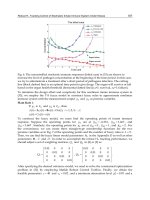
results of the formulation are presented in the following section.

The equations 1 - 6 from the previous section are the same also for the query-based information
gathering.
116
Mobile Ad-Hoc Networks: Applications
yTra f fic Information Dissemination in Vehi cular Ad Hoc Networks 11
In order to find an optimal point to send a query message, we have to define the following set
of variables:
– s
nm
ij
is 1 if edge ij belongs to the common part of the normal and the by-pass route and to
the DoI as well.
With the following three constraints the properties of variables s
nm
ij
are ensured:
For each n, m
∈Vwhere OD(n, m) > 0:
r
ij
≥ b
nm
ij
+ s
nm
ij
(9)
s
nm
ij

≤ a
nm
ij
(10)
Edges where s
nm
ij
or b
nm
ij
takes value 1 should be a coherent region, which ends at the traffic
jam:
∑
i∈V
(s
nm
ij
+ b
nm
ij
) −
∑
k∈V
(s
nm
jk
+ b
nm
jk
)=


1if
∃kc
nm
jk
= 1
≤ 0otherwise
Finally, the propagation delay of the distributed messages has to be taken into account. It
takes some time for the query message to reach the jam, and the reply message to reach the
originator. The query message should reach the begin of jam, collect information and the reply
message should reach the vehicle before it reaches the optimal decision point expressed by the
following constraint:
∑
(i,j)∈V
(s
nm
ij
l
ij
v
veh
− (2b
nm
ij
+ s
nm
ij
)
l
ij

v
mess
) ≥ 0, (11)
Where l
ij
is the length of the ij road segment, v
veh
is the velocity of the vehicle, v
mess
is the
velocity of the message propagation.
Finally, we define the objective by minimizing the weighted average of the length of all
by-pass routes and the total length of the DoI:
min
∑
(i,j)∈E

αl

ij
∑
n,m∈V
y
nm
ij
+(1 − α)l

ij
r
ij


(12)
where, l

ij
is the cost (length, travel time, etc.) of traveling on road (i, j) while l

ij
denotes the cost
(e.g., road length, communication cost) of propagating information on road
(i, j). Parameter
α (0
≤ α ≤ 1) expresses the importance of minimizing the total length of all by-pass routes
against the total DoI.
In the next section, we use this formulation as follows. First, for each n, m
∈V where
OD
(n, m) > 0 calculate shortest path and set variables x
nm
ij
based on the result of the shortest
path algorithm. Second, solve the following ILP problem: constants: x
nm
ij
, c
nm
ij
, l

ij

, l

ij
;binary
variables: y
nm
ij
, r
ij
, a
nm
ij
, b
nm
ij
, d
nm
ij
, f
nm
ij
, objective: (12) and constraints: (2)-(6) and (9)-(11).
4. Numerical analysis of the SPACE and SPACE ILP algorithms
In this section we present the evaluation of the proposed heuristic and linear programming
algorithms. All the simulations were effectuated on the same section of a digital map of
Budapest.
117
Traffic Information Dissemination in Vehicular Ad Hoc Networks
12 Theory and Applications of Ad Hoc Networks
4.1 SPACE

The output of the SPACE algorithm is demonstrated on Figure 3 for two roads of the Budapest
test network. A main road (bridge, solid line), and a side road (from down-town, dotted line)
were considered for analysis. The x-axis represents the domain of interest, i.e., the sum of
road lengths on which the information about the event is disseminated, while y-axis represent
the impact factor. The information is sent to roads (e) of higher impact factors (I
E
f
(e)), while
roads with minor impact factors can be neglected. First, we assume that there is a traffic jam
(obstacle) on the main road (depicted with solid line). If the TTI information is flooded to the
whole domain of interest, then it should be spread to 16,000 meters. Therefore, a threshold
(e.g., TR = 4,000) should be set in order to avoid superfluous forwarding. In this way the
information is carried to the majority of vehicles (just 1,000 from more than 15,000 do not
receive the information in time), while the domain of interest is decreased to 4,000 meters,
instead of 16,000. Second, we consider an obstacle on a side street (dashed line). As expected,
the impact factor of such streets is less, i.e., if the threshold is set to 1,000 then the domain of
interest is 500 meters.
Fig. 3. Domains of Interest for different road types using the SPACE algorithm
4.2 SPACE ILP
In order to have a better understanding, the results of the SPACE ILP algorithm are presented
below. A main road ( bridge), and different side roads (from downtown area) were considered
for analysis. The bridge graph represents averaged values for traffic demands initiated from
both sides of the city, considering traffic jam on one of the bridge lanes. The downtown graph
represents averaged values from different congested downtown roads (considering also the
major roads leading to the bridge).
Figure 4 shows the Domain of Interest (DoI) depending on the parameter α (see Objective
(8)). We recall that α (0
≤ α ≤ 1) expresses the importance of minimizing the total length of
all vehicle by-pass routes against the importance of minimizing the propagation region (area
of dissemination). The DoI is represented as the sum of the road segment lengths included in

the propagation region.
It is obvious that for both graphs the DoI increases by increasing α. On the other hand, the
figure shows that the two types of roads represent different dynamics considering their DoI.
In case when the obstacle is on the bridge, the DoI increases steeply with the increase of α.This
means that in order to reach all roads of the maximum DoI, higher efforts must be involved for
TTI dissemination. However, after a limit (α
≥ 0.6) the DoI is not increasing significantly (only
about 1 km). A crucial point for α is between 0.3 - 0.4, where the DoI increases significantly.
Considering congestion on downtown roads the situation is different. It can be s een, that the
118
Mobile Ad-Hoc Networks: Applications
yTra f fic Information Dissemination in Vehi cular Ad Hoc Networks 13
Fig. 4. Domains of interest in function of parameter α
variance of the DoI values is higher; however, the area of DoI for downtown scenarios is only
a fraction of the values of the bridge scenarios.
These observations are also validated if we consider the length of alternative (by-pass) routes
in function of α (Figure 5). As α increases, the length of by-pass routes will decrease, because
more and more vehicles will be able to choose the ideal by-pass routes to avoid the congestion.
For the bridge scenario the length of alternative routes decreases with about 30% if we
disseminate TTI by employing α = 0.4. In case of downtown congestions, we can observe
that the length of alternative routes will not decrease significantly as we increase α,sincethe
best by-pass routes are closer to the area of congestion. Thus, for downtown roads it is useless
to disseminate the information further than the next couple of road segments (e.g. 200-300
meters), since the by-pass routes would not become shorter in any case.
Numerous analysis have been carried out that also show that the effect of α on the DoI and
length of alternative routes is significant between 0.2 and 0.4 for most of the roads.
4.3 Query-based information gathering
In this section we present the n umerical results of the generic query-based traffic information
gathering protocol. The results were generated by creating a large amount of random
source-destination route pairs on the road graph of Budapest. Optimal query locations were

generated by solving the ILP formulation described in the previous section. A characteristic
set of results, presenting interesting cases, were selected for presentation.
On Figure 6 the x-axis represents the distance of the source (n) of a vehicle from the traffic jam
(while the destination (m) was fixed), while the y-axis represents the alteration in length of
the respective metrics. The road length increase presents the difference between the original
and the different by-pass routes (
∑
(i,j)∈E
l

ij
(y
nm
ij
− x
nm
ij
),forsourcen and destination m), while
the query distance metric presents the distance from where the query is injected towards the
point of i nterest (
∑
(i,j)∈E
(l

ij
r
ij
), l

ij

= l

ij
= length of road (i, j)).
In case when the jam was on a bridge (diagrams noted with (B)), the length of the original
route was 3300 meters. When the distance was less than 200 meters from the traffic incident,
the increase in the by-pass route length was nearly 1600 meters, an increase of around 50% of
119
Traffic Information Dissemination in Vehicular Ad Hoc Networks
14 Theory and Applications of Ad Hoc Networks
Fig. 5. Length of alternative routes in function of parameter α
the original route. As the source was generated further away from the traffic jam, the by-pass
route length increase could be reduced significantly. The breakpoints in the graph are the
points in the road network, where a new by-pass route could be taken. As we can see, the
optimal query distance in this case is around 1000 meters. That is the point where the vehicles
can take the shortest by-pass route according to the information contained in the returned TTI
message.
On the diagrams noted with (M2), a major road in the city is displayed, where the length of
the original route was 2500 meters. It can be seen that in case of short query distances the
length of the by-pass routes could be as much as the double of the original route length. As
the query distance is increased to 1000 meters, the by-pass route length decreases to around
600 meters, and with a query distance of 1200 meters, the route length increase is only 100
meters. This shows that finding the optimal query distance is really important, because the
length of the by-pass route can be reduced significantly.
The diagrams noted with (M1) present a case when the traffic jam is on a main downtown road
with plenty of nearby roads, which can be taken as by-pass routes. Thus, the query distance
can be set to a small value, since the increase in by-pass route will become negligible.
4.4 Comparison of SPACE and SPACE ILP
Until now we investigated the effect of traffic congestion on TTI dissemination separately
studying the heuristic (SPACE) and the optimal (SPACE

ILP) Domain of Interest calculation
algorithms. Considering the results from Section 4.1 and Section 4.2 we can affirm that the
outcome of the algorithms present certain similarities. For example, from both approaches
it turns out that the traffic jams can be classified in two major categories. One category
is represented by traffic jams of main, crucial roads (e.g. bridge), with a large Domain of
Interest and an increased length of the by-pass routes. The dissemination of TTI for such
traffic incidents is extremely important, since the zone of no return of these traffic jams is also
large. The second category of traffic jams is represented by downtown roads with small DoI
120
Mobile Ad-Hoc Networks: Applications